

Abstract
We developed a deep learning–based super-resolution model for prostate MRI. 2D T2-weighted turbo spin echo (T2w-TSE) images are the core anatomical sequences in a multiparametric MRI (mpMRI) protocol. These images have coarse through-plane resolution, are non-isotropic, and have long acquisition times (approximately 10–15 min). The model we developed aims to preserve high-frequency details that are normally lost after 3D reconstruction. We propose a novel framework for generating isotropic volumes using generative adversarial networks (GAN) from anisotropic 2D T2w-TSE and single-shot fast spin echo (ssFSE) images. The CycleGAN model used in this study allows the unpaired dataset mapping to reconstruct super-resolution (SR) volumes. Fivefold cross-validation was performed. The improvements from patch-to-volume reconstruction (PVR) to SR are 80.17%, 63.77%, and 186% for perceptual index (PI), RMSE, and SSIM, respectively; the improvements from slice-to-volume reconstruction (SVR) to SR are 72.41%, 17.44%, and 7.5% for PI, RMSE, and SSIM, respectively. Five ssFSE cases were used to test for generalizability; the perceptual quality of SR images surpasses the in-plane ssFSE images by 37.5%, with 3.26% improvement in SSIM and a higher RMSE by 7.92%. SR images were quantitatively assessed with radiologist Likert scores. Our isotropic SR volumes are able to reproduce high-frequency detail, maintaining comparable image quality to in-plane TSE images in all planes without sacrificing perceptual accuracy. The SR reconstruction networks were also successfully applied to the ssFSE images, demonstrating that high-quality isotropic volume achieved from ultra-fast acquisition is feasible.
Keywords: Super-resolution, Prostate MRI, Generative adversarial network, Image quality
Introduction
Multiparametric magnetic resonance imaging (mpMRI) is becoming standard practice for the diagnosis and risk stratification of prostate cancer. The typical mpMRI protocol consists of anatomical and functional sequences, which can be used for staging cancer and selecting regions of interest for targeted biopsy [1–4]. The anatomical sequences include high-resolution (HR) axial, sagittal, and coronal T2-weighted turbo spin echo (T2w-TSE) images and the functional sequences include diffusion-weighted (DW) and dynamic contrast-enhanced (DCE) images [5]. On average, T2w-TSE, DW, and DCE sequences take approximately 10–15 min, 5 min, and 5 min respectively. T2w-TSE images therefore account for roughly 60% of the total mpMRI acquisition time [6]. This long acquisition time is not only time-consuming but also uncomfortable for the patient. Accelerated MR imaging to shorten acquisition time especially for body and pelvis imaging has been studied intensively. A single 3D (volumetric) scan can be acquired in roughly half the time of multi-plane 2D scans. 3D acquisitions however are more prone to motion artifacts and exhibit weaker T2 contrast [6–9]. Acquisition time can also be significantly reduced by ultra-fast 2D sequences, such as single-shot fast spin echo (ssFSE) acquired in orthogonal planes, which would be 10 times faster than the standard orthogonal-plane TSE scans. Ultra-fast sequences produce low-resolution (LR) images that need to be post-processed to form high-resolution (HR) images via super-resolution (SR) techniques. In this study, we used deep learning–based SR technique to restore HR features from ultra-fast LR images; therefore, HR images can be generated with reduced acquisition time.
Related Works
Traditional interpolation methods such as nearest neighbor, bilinear, and bicubic interpolations can render smooth images from LR images. Slice-to-volume reconstruction (SVR) and patch-to-volume reconstruction (PVR) are two methods that integrate axial, coronal, and sagittal images into an isotropic 3D volume with B-spline interpolation and maximum likelihood super-resolution [10, 11]. SVR and PVR volumes are insensitive to motion but induce artifacts. Recently, deep learning models have been used to generate SR images. Specifically, generative adversarial networks (GAN) are known for generating high-fidelity SR images [12, 13]. Ledig et al. [12] used GAN with perceptual loss and He et al. [14] used an attention model to achieve high-quality SR images. In order to train and test SR networks, LR images are simulated from HR images. He et al. [14] used bicubic interpolation and Lyu et al. [15] discarded 75% of the peripheral region in the frequency domain to synthetically generate LR images. However, SR networks trained with certain simulated LR images tend to learn the specific pattern associated with the downsampling method. Without using simulation techniques, Sood and Rusu [16] used real anisotropic MR through-plane as LR images for their 2D GAN. However, HR-LR pair images are required for their network architecture. All the above SR approaches generate 2D images that improve in-plane resolution with anisotropic voxel size in the slice direction. Our approach provides a way to generate isotropic SR 3D volume which can be reformatted in any plane.
This work proposes the use of 3D reconstructed images (Fig. 1a) instead of simulated LR images as low-resolution (LR) data inputs to convolutional neural networks (CNNs). With 3D reconstruction, a single isotropic volume can be created from multiplanar 2D images, reducing partial volume effects. 3D volumes, however, display image quality degradation due to high-frequency signal loss and stripe artifacts (Fig. 1b). To restore image resolution and T2 contrast, we propose the use of GANs (Fig. 1c). Previous SR CNNs require paired high-resolution ground-truth (GT) images and downsampled LR images [17]. In this study, extra interpolated slices were generated in the reconstruction process (Fig. 2). Though unpaired data is normally discarded in paired supervised networks, the CycleGAN [18] (an extension of conventional GAN) does not require paired data and can conquer this limitation. We, therefore, implemented three CycleGAN networks for axial, coronal, and sagittal T2w-TSE images with resliced SVR volumes. The networks map LR slices to T2-w TSE GT images in an unpaired manner.
Fig. 1.

Axial view of a 2D T2-weighted TSE image, b 3D slice-to-volume reconstructed (SVR) image, and c CycleGAN-SR image. The white arrow in b indicates a stripe artifact in the SVR image
Fig. 2.
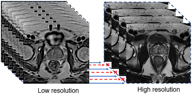
Slice-to-volume reconstructed (SVR) low-resolution volumetric image with 0.75-mm slice thickness and high-resolution T2w-TSE image with 3.6-mm slice thickness. Extra interpolated slices in the SVR volume have no paired HR T2w-TSE slices, as indicated by the red dashed arrow. In this case, unpaired learning is used
Methods
Patient Data
Three hundred forty-six patients and their associated three-plane T2w-TSE scans from the ProstateX grand challenge [19] were used. The images were acquired at a single institution on two Siemens 3-T MRI scanners (MAGNETOM Trio, Magnetom Skyra). T2w-TSE sequences with 0.5-mm in-plane resolution and 3.6–mm slice thickness were acquired. These images were subsequently reconstructed into isotropic volumes with a voxel size of 0.75 × 0.75 × 0.75 mm3 using SVR and PVR techniques proposed by Alansary et al. [10] A fivefold cross-validation was performed across the complete dataset, and no additional testing set was reserved due to the small dataset size.
Additionally, five cases with three-plane single-shot fast spin echo (ssFSE) were acquired at our institution (3 T Discovery 750 W, GE Healthcare) to evaluate the generalizability of the networks. Images were acquired with 0.8 × 0.8 mm2 in-plane resolution and 4-mm slice thickness. 3D isotropic HyperCube (0.6 × 0.6 × 0.6 mm3) volumes were also acquired from the same patients to use as isotropic reference images.
The workflow to generate SR volumes is summarized in Fig. 3. Axial, coronal, and sagittal T2w-TSE images were first combined into a single isotropic volume using SVR. The SVR volumes were then resliced to form axial, coronal, and sagittal LR images. These LR images were trained with 2D TSE slices as GT.
Fig. 3.

Workflow for generating super-resolution (SR) volumes. PVR/SVR volumes were resliced into 2D slices to perform slice-to-slice SR training for axial, coronal, and sagittal planes. The SR algorithm is trained jointly with T2-weighted images as ground truth. Three stacks of SR slices were reconstructed into SR 3D isotropic volume
Pre-processing
CycleGAN’s ability to utilize unpaired data enables the whole dataset training without discarding any misaligned slices (Fig. 2). To ensure that real details from GT images are restored in the generated SR images, CycleGAN introduces another CNN to translate SR images back to the LR domain. This additional CNN ensures cycle consistency by minimizing differences between the reconstructed images and original SVR images.
For each patient, N4 normalization was first applied to T2w-TSE images to correct for intensity non-uniformity [20]. The SVR volume was then resliced into stacks of 2D images in axial, coronal, and sagittal directions, forming 3 separate datasets: T2w-TSE as GT and SVR as LR. During the training phase, all 2D images were resampled to 286 × 286 pixels, and a random crop of 256 × 256 pixels was applied on-the-fly. Central crops of 150 × 150 pixels zoomed in the prostate region and scaled back to 256 × 256, along with rotation and vertical flipping, were used to augment the data.
Network Architecture
SR images were achieved as a domains mapping process from LR data to HR data. The SR images were generated from the CycleGAN model, which consists of two pairs of generative adversarial networks. Two generators were also used to reconstruct images as described in Fig. 4.
Fig. 4.

The network architecture of CycleGAN. CycleGAN generates SR images based on a GAN model, as indicated in the red-dashed box. Cycle consistency can be achieved by introducing another generator (GLR(Generated SR)) to convert the SR images back to the original LR domain in order to minimize differences between the LR SVR and reconstructed LR images. A backward loop including GLR(GT TSE), DLR, and GGT(Generated LR) is also established to maintain the balance of the CycleGAN network
Typically, a GAN consists of a generator that generates data which a discriminator cannot distinguish from the real data [21]. Since a discriminator ensures the likeness of generated data with the original data, the reliability of the generated data depends heavily on the performance of the discriminator. In addition to a conventional GAN architecture (enclosed by the red dotted line in Fig. 4), the CycleGAN also includes a generator to translate the generated data back to the original data domain. By minimizing the differences between the reconstructed data and the original data, which is called cycle-consistency loss, a second constraint has been enforced on the model to prevent deviation of generated data from ground truth.
Assuming there are n samples {LR(1),…, LR(j),…, LR(n)} of LR slices and m samples {GT(1),…, GT(i),…, GT(m)} of GT slices, the generator loss in the LR to GT direction is expressed as:
| 1 |
where denotes the j-th LR slices, represents the generated SR image by generator from , and represents the discriminator that is trying to discriminate between the generated SR image and GT image. If the discriminator cannot distinguish the generated SR image from the GT image, DGT = 1. This means that the discriminator views the generated image as the ground-truth image; otherwise, a 0 label is given. The aims to minimize the generator loss (Eq. 1) by producing images as close to the ground-truth images as possible so that the discriminator labels the generated image as 1 (DGT = 1).
The discriminator loss in the LR to GT direction is expressed as:
| 2 |
where denotes the i-th GT slices, represents the j-th LR slices, represents the generated SR image by generator from , and represents the discriminator that is trying to identify the generated image from GT images. If the discriminator cannot distinguish the generated image from the GT image, = 1, which means that the discriminator recognizes the generated image as the GT image; otherwise, a 0 label is given. The aims to minimize the discriminator loss (Eq. 2) by recognizing the generated images (labeled as 0) and correctly identifying the ground-truth images (labeled as 1).
The adversarial loss of the LR to GT direction is the summation of the generator loss and the discriminator loss, as expressed in Eq. 3.
| 3 |
The adversarial loss of GT to LR direction is similar to Eq. 3 with replacing .
When SR images were generated by , an extra generator was simultaneously trained to translate the SR images back to the LR domain. These translated images are called reconstructed images, expressed in Eq. 4:
| 4 |
By minimizing the error between the ground-truth image and the reconstructed image, cycle consistency is achieved. Similar to the adversarial loss in the CycleGAN model, the cycle consistency loss can be obtained in both directions: LR → GT → LR and GT → LR → GT. The cycle consistency loss for LR → GT → LR is expressed in Eq. 5. The loss of GT → LR → GT direction is analogous.
| 5 |
Network Implementation and Training
The generators consist of 2 stride-2 convolutions, 9 residual net blocks, 2 stride- convolutions, and batch normalization. The discriminators are Markovian discriminators known as PatchGAN [22], consisting of 4 stride-2 convolutions, 2 stride-1 convolutions, and batch normalization. The model as a whole was trained with randomly selected unpaired data using ADAM optimizer with the initial learning rate of 0.0002 and a 50% dropout rate to prevent overfitting. A total of 200 epochs were trained with a batch size of 6 on 4 NVIDIA GeForce GTX 1080 Ti GPUs.
In the training phase, the GGT learns to translate SVR slices to TSE-like slices and DGT learns to distinguish the generated output from TSE slices. By distinguishing the output of GGT, DGT acts as a loss function to provide improved direction to GGT.
Post-process
After the axial, coronal, and sagittal networks were trained, the weights were applied to the SVR images. For each patient, the predicted SR 2D images were stacked to reconstruct isotropic 3D volumes forming 3 volumes for each anatomical view. The 3 SR volumes of each patient were registered to the axial volume using the symmetric normalization non-linear registration algorithm known as SyN [23]. The axial volume and registered coronal and sagittal volumes were averaged together to generate a final 3D SR volume.
For evaluation, the identical SR technique was applied to the ssFSE images for testing the generalizability of networks. Next, the PVR, SVR, and our SR and ssFSE volumes were rigidly registered to HyperCube volumes in order to undergo evaluation procedures.
Quantitative Evaluation
Recently, there have been concerns regarding the ability of conventional quantitative evaluation metrics such as mean absolute error (MAE), root-mean-squared error (RMSE), peak signal-to-noise ratio (PSNR), and Structural Similarity Index (SSIM) to evaluate the image quality of GAN-based SR images. In an in-depth review published by Yi et al. [24] discussing state-of-the-art GAN models being applied in medical images, the authors found that MAE, PSNR, and SSIM do not correspond to the visual quality of images. For example, even when direct optimization of pixel-wise loss produces a more visually blurry image than adversarial loss, the direct optimization of pixel-wise loss always yields higher numbers for PSNR and SSIM.
Therefore, along with RMSE (Eq. 6), PSNR (Eq. 7), and SSIM (Eq. 8), two additional metrics — perceptual index (PI) [25] (Eq. 9) and the radiologist Likert scores — were introduced in this study for SR image evaluation to yield a better understanding of the realistic image quality compared to conventional metrics.
The RMSE is defined as:
| 6 |
where n denotes the total pixel count of an image, i denotes the i-th pixel, denotes the intensity value of the i-th pixel in ground-truth images, and denotes the intensity value of i-th pixel in super-resolution images.
The PSNR is defined as:
| 7 |
where is the maximum pixel value in the SR image and MSE is the mean squared error between the GT and SR images.
The structural similarity index between two images is defined as:
| 8 |
where (x, y) denotes two input matrices, (μx, μy) denotes the average of x and y, (σx, σy) denotes the variance of x and y, σxy denotes the covariance of x and y, L denotes the maximum possible bit depth value in (x, y) matrix (e.g., 255 for 8-bit images (2D matrix)), and k1 = 0.01 and k2 = 0.03 by default.
The PI [25] is an image quality metric which does not rely on the ground-truth reference image. The 2018 PIRM challenge [25] defines PI as the combination of two non-reference image quality regression models: Ma et al. [26] and the Natural Image Quality Evaluator (NIQE) index [27].
| 9 |
Ma et al. [26] followed the image quality assessment (IQA) methodology [28] to conduct a human visual study to quantify perceptual quality of SR images generated by 9 different algorithms. The NIQE index is a blind IQA multivariate Gaussian model that characterizes image natural scene statistics (NSS) in the space domain. The NSS features can be extracted from the test images and compared with the Gaussian model to generate a NIQE score. Notice that a lower PI score indicates better perceptual quality.
The radiologist Likert score is defined as a 4-point scoring system. We adopted the recommendations from the prostate imaging-reporting and data system to assess the diagnostic quality of prostate MR images with 5 criteria [29]. The reviewing criteria include whether or not the capsule, seminal vesicles, neurovascular bundles, and sphincter muscle are clearly delineated and the ability to distinguish central/peripheral zones. A score of 1 indicates insufficient delineation, a score of 2 indicates adequate delineation, a score of 3 indicates good delineation, and a score of 4 indicates excellent delineation. An average score is obtained from all 5 criteria to represent overall diagnostic image quality.
Results
SR slices were post-processed into a single SR volume with 0.75 × 0.75 × 0.75 mm3 voxel size. The results of cross-validation of T2-w TSE images from ProstateX challenge were reported. Five cases of ssFSE images were also tested to gauge generalizability of the networks. In order to obtain an optimized result when testing the ssFSE dataset, an early stopping was applied to the axial network at epoch 63; coronal network at epoch 63; sagittal network at epoch 69.
ProstateX Dataset
Figure 5 shows the 3D reconstruction results of T2-weighted TSE images from the ProstateX challenge. The PVR volume (Fig. 5a, e, i) has the smallest field-of-view (FOV) and is the most severely degraded reconstructed volume. The SVR volume (Fig. 5b, f, j) shows moderate degradation compared to in-plane TSE images (Fig. 5d, h, l) but has uniform image quality in all three planes. Our SR volume (Fig. 5c, g, k) has slightly degraded image quality compared to in-plane TSE views but superior image quality compared to TSE out-of-plane views. Although the axial in-plane T2-w TSE (Fig. 5d) serves as the GT image, its out-of-plane images (Fig. 5h, l) suffer from suboptimal quality with blurry and poorly defined prostate peripheral edges.
Fig. 5.

3D reconstruction results of T2-weighted TSE images from ProstateX challenge (no. 319 central slices). d, h, and l show axial TSE images with anisotropic voxel size, which gives better in-plane axial image quality, and poorer coronal and sagittal out-of-plane image quality. a, e, and i show isotropic 3D volumes reconstructed by PVR method. b, f, and j show isotropic 3D volumes reconstructed by SVR method. c, g, and k show isotropic 3D volumes reconstructed by our SR method
Quantitative evaluation of the TSE cases (ProstateX dataset) was performed using the corresponding in-plane slice of T2-w TSE images as a reference image against different reconstruction methods in the two-dimensional base. The central slice of each case was extracted for the comparison, and the results of PI, RMSE, and SSIM are displayed in Table 1. The improvements from PVR to SR are 80.17%, 90.28%, 63.77%, and 186% for PI, PSNR, RMSE, and SSIM, respectively; the improvements from SVR to SR are 72.41%, 2.35%, 17.44%, and 7.5% for PI, PSNR, RMSE, and SSIM respectively. Sood and Rusu [16] also used the ProstateX dataset with a SRGAN and achieved 21.27 PSNR and 0.66 SSIM at the × 4 downsampling set.
Table 1.
PI, PSNR, RMSE, and SSIM for ProstateX TSE cases (results are expressed as the average value ± one standard deviation)
| ProstateX dataset | ||||
|---|---|---|---|---|
| Images | PI | PSNR | RMSE | SSIM |
| PVR | 12.63 ± 0.37 | 15.34 ± 0.21 | 78.77 ± 0.93 | 0.31 ± 0.09 |
| SVR | 9.08 ± 0.09 | 28.52 ± 0.38 | 34.57 ± 0.45 | 0.84 ± 0.07 |
| SRGAN [16] | - | 21.27 | - | 0.66 |
| Our SR | 2.50 ± 0.02 | 29.19 ± 0.32 | 28.54 ± 0.31 | 0.90 ± 0.02 |
ssFSE Dataset
The perceptual quality of our SR images surpasses that of the in-plane ssFSE images by 37.5% while the RMSE is slightly higher by 7.92% (Fig. 6 and Table 2). The isotropic SR images display better image contrast and image resolution than ssFSE images. Therefore, a 3D isotropic volume (HyperCube) acquired from the same patient, instead of an anisotropic ssFSE image, was used as the reference image for evaluation purposes. The evaluation can be performed in a three-dimensional base because the HyperCube volumes have uniform image qualities throughout all three planes. Perceptual index, however, was calculated in 2D central slices in accordance with the 2D algorithm provided by the 2018 PIRM challenge. We found that after a certain number of epochs (approximately 60 epochs), the testing loss of ProstateX dataset still decreased while the testing loss of ssFSE dataset reached the minimum and started to increase. This is because the network became more and more specific to the dataset it was trained on and gradually lost its generalizability.
Fig. 6.

3D reconstruction results of ssFSE images. d, i, and n show axial ssFSE images with anisotropic voxel size, which gives better in-plane axial image quality, and poorer coronal and sagittal out-plane image quality. a, f, and k show isotropic 3D volumes reconstructed by PVR method. b, g, and l show isotropic 3D volumes reconstructed by SVR method. c, h, and m show isotropic 3D volumes reconstructed by our SR method. e, j, and o show high-resolution 3D HyperCube isotropic volumes acquired from patients as the reference images
Table 2.
PI, PSNR, RMSE, and SSIM for ssFSE cases (results are expressed as the average value ± one standard deviation)
| ssFSE dataset | ||||
|---|---|---|---|---|
| Images | PI | PSNR | RMSE | SSIM |
| PVR | 12.74 ± 0.12 | 15.35 ± 0.25 | 44.27 ± 0.73 | 0.65 ± 0.09 |
| SVR | 7.83 ± 0.05 | 28.41 ± 0.47 | 27.84 ± 0.46 | 0.68 ± 0.05 |
| Our SR | 2.48 ± 0.09 | 27.47 ± 0.28 | 30.49 ± 0.35 | 0.78 ± 0.03 |
Figure 6 shows the 3D reconstruction results of ssFSE images. Three isotropic images with 0.75 × 0.75 × 0.75 mm3 voxel size, namely PVR, SVR, and SR, were generated from ssFSE images; and therefore, these images have uniform image qualities throughout three different views. The Hypercube images, acquired along with the ssFSE images, were also included in the evaluation to establish a standard image quality score for comparison. The results of the quantitative analysis are displayed in Table 2. The SR volume scored a perceptual index of 2.48, which is higher than the ssFSE (3.41), HyperCube (4.67), SVR (7.83), and PVR (12.74). The lowest PI indicates that the SR volume has the best perceptual accuracy in the human visual system among other comparison images. Compared with the ground-truth images (HyperCube), the SVR images have the lowest RMSE value (27.84), followed by ssFSE (28.25), SR (30.49), and PVR (44.27). For structure similarity, the SSIM for SR volume is the highest (0.78), followed by the ssFSE (0.76), SVR (0.68), and PVR (0.65).
Radiologist Likert Scores
The Likert scores were provided by a board-certified body radiologist after reviewing 12 randomly selected cases. Scores for TSE, SR, and SVR images are displayed in Table 3. PVR images were not reviewed by the radiologist because of inadequate FOV coverage to the prostate and adjacent tissues-of-interest. TSE images and SR volumes both achieved scores above 3 in the overall image quality and each individual assessment criterion whereas SVR volumes achieved scores around 2. For overall image quality, SR volumes scored 38% higher to SVR volumes. Isotropic SR volumes provide uniform image quality across different planes which allow radiologists to access 3-dimensional diagnostic information. Structures such as prostate central zone, peripheral zone, transition zones, and periurethral glands can be more clearly distinguished when reviewing SR volumes.
Table 3.
Radiologist Likert scores (results are expressed as the average value ± one standard deviation; score 1, insufficient; score 2, adequate; score 3, good; score 4, excellent)
| Capsule clearly delineated | Seminal vesicles clearly delineated | Neurovascular bundles clearly delineated | Sphincter muscle clearly delineated | Ability to distinguish central/peripheral zones | Overall image quality | |
|---|---|---|---|---|---|---|
| TSE | 3.83 ± 0.39 | 3.83 ± 0.39 | 3.75 ± 0.62 | 3.83 ± 0.39 | 3.83 ± 0.39 | 3.81 ± 0.42 |
| SR | 3.00 ± 0.60 | 3.17 ± 0.38 | 3.00 ± 0.43 | 3.33 ± 0.65 | 3.33 ± 0.65 | 3.11 ± 0.41 |
| SVR | 2.33 ± 0.49 | 2.41 ± 0.51 | 2.16 ± 0.57 | 2.58 ± 0.51 | 2.41 ± 0.51 | 2.25 ± 0.38 |
Discussion
In order to compute RMSE, PSNR, and SSIM scores, the PVR, SVR, and SR images must be registered with the ground-truth image and cropped to identical sizes. Even with rigid registration, images may still be distorted, which can affect RMSE and SSIM scores. Perceptual index (PI) yields more accurate results since it is a non-reference metric simulating the human visual system and needs no extra procedures to evaluate image quality.
GAN-based SR images can appear realistic with high perceptual quality and yet have a weak relationship with ground-truth images. Plotting RMSE vs PI allows us to visualize reconstruction accuracy vs perceptual image quality (Fig. 7). In Fig. 7, proximity to the origin indicates better perceptual quality and less image distortion, or better image quality. Figure 7 visualizes the change in image quality during the SR reconstruction processes outlined in Fig. 3. The isotropic volumes (ProstateX PVR, SVR, and ssFSE PVR, SVR) suffer from PI and RMSE degradation to different degrees as indicated in Fig. 7. The ProstateX SR volumes demonstrate the ability to restore image quality with high reconstruction accuracy and high perceptual quality; the ssFSE SR volumes also demonstrate significant perceptual quality improvements compared to the SVR reconstruction method.
Fig. 7.

Evaluation results in the perception-distortion plane. Each image is a point on the perception-distortion plane, whose axes are the RMSE and PI. The perceptual quality of the SR images (ProstateX SR and ssFSE SR) significantly increased while the RMSE scores remained comparable to that of SVR images. Notice that the ssFSE and the ssFSE SR images are very close to each other, which indicates that the SR reconstruction process does not sacrifice image quality
Since the perceptual quality of ssFSE SR volumes (Fig. 6 SR) surpasses that of the ssFSE images (Fig. 6 ssFSE) especially for out-of-plane slices, we switched the GT images from ssFSE images to HyperCube volumes (Fig. 6 HyperCube) acquired from the same patient in order to perform quantitative evaluation with reasonable results.
Conclusion
T2-weighted TSE images have fine in-plane resolution but suboptimal out-of-plane resolution. The PVR and SVR reconstructed 3D volumes have isotropic voxel size but degraded image quality compared to in-plane T2-w TSE images. Our proposed SR method achieves isotropic SR volumes (with 0.75 × 0.75 × 0.75 mm3 voxel size) without sacrificing reconstruction and perception accuracy. The SR networks restore the high-resolution features learned from axial, coronal, and sagittal in-plane TSE images. Despite being trained on ProstateX data, the networks managed to generate high-quality isotropic SR volumes on the ssFSE (one-tenth of the scan time of conventional three-plane TSE scans) dataset as well, which demonstrates generalizability of the network. Diagnostic quality assessment by an experienced radiologist also indicates good overall image quality of our 3D SR volumes.
Declarations
Conflict of Interest
The authors declare no competing interests.
Footnotes
Publisher's Note
Springer Nature remains neutral with regard to jurisdictional claims in published maps and institutional affiliations.
References
- 1.Ghai S, Haider MA. Multiparametric-MRI in diagnosis of prostate cancer. Indian J. Urol. 2015;31:194–201. doi: 10.4103/0970-1591.159606. [DOI] [PMC free article] [PubMed] [Google Scholar]
- 2.Fütterer JJ, et al. Can Clinically Significant Prostate Cancer Be Detected with Multiparametric Magnetic Resonance Imaging? A Systematic Review of the Literature. Eur. Urol. 2015;68:1045–1053. doi: 10.1016/j.eururo.2015.01.013. [DOI] [PubMed] [Google Scholar]
- 3.Tsai WC, Field L, Stewart S, Schultz M. Review of the accuracy of multi-parametric MRI prostate in detecting prostate cancer within a local reporting service. J. Med. Imaging Radiat. Oncol. 2020 doi: 10.1111/1754-9485.13029. [DOI] [PubMed] [Google Scholar]
- 4.Stabile A, et al. Multiparametric MRI for prostate cancer diagnosis: current status and future directions. Nat. Rev. Urol. 2020;17:41–61. doi: 10.1038/s41585-019-0212-4. [DOI] [PubMed] [Google Scholar]
- 5.Bittencourt LK, de Hollanda ES, de Oliveira RV. Multiparametric MR Imaging for Detection and Locoregional Staging of Prostate Cancer. Top. Magn. Reson. Imaging. 2016;25:109–117. doi: 10.1097/RMR.0000000000000089. [DOI] [PubMed] [Google Scholar]
- 6.Polanec SH, et al. 3D T2-weighted imaging to shorten multiparametric prostate MRI protocols. Eur. Radiol. 2018;28:1634–1641. doi: 10.1007/s00330-017-5120-5. [DOI] [PMC free article] [PubMed] [Google Scholar]
- 7.Rosenkrantz AB, et al. Prostate cancer: Comparison of 3D T2-weighted with conventional 2D T2-weighted imaging for image quality and tumor detection. AJR Am. J. Roentgenol. 2010;194:446–452. doi: 10.2214/AJR.09.3217. [DOI] [PubMed] [Google Scholar]
- 8.Westphalen AC, et al. High-Resolution 3-T Endorectal Prostate MRI: A Multireader Study of Radiologist Preference and Perceived Interpretive Quality of 2D and 3D T2-Weighted Fast Spin-Echo MR Images. AJR Am. J. Roentgenol. 2016;206:86–91. doi: 10.2214/AJR.14.14065. [DOI] [PMC free article] [PubMed] [Google Scholar]
- 9.Caglic I, et al. Defining the incremental value of 3D T2-weighted imaging in the assessment of prostate cancer extracapsular extension. Eur. Radiol. 2019;29:5488–5497. doi: 10.1007/s00330-019-06070-6. [DOI] [PMC free article] [PubMed] [Google Scholar]
- 10.Alansary A, et al. PVR: Patch-to-Volume Reconstruction for Large Area Motion Correction of Fetal MRI. IEEE Trans. Med. Imaging. 2017;36:2031–2044. doi: 10.1109/TMI.2017.2737081. [DOI] [PMC free article] [PubMed] [Google Scholar]
- 11.Uus A, et al. Deformable Slice-to-Volume Registration for Motion Correction of Fetal Body and Placenta MRI. IEEE Trans. Med. Imaging. 2020 doi: 10.1109/TMI.2020.2974844. [DOI] [PMC free article] [PubMed] [Google Scholar]
- 12.Ledig, C. et al. Photo-realistic single image super-resolution using a generative adversarial network. InProceedings of the IEEE conference on computer vision and pattern recognition 4681–4690 (2017).
- 13.Lyu, Q., You, C., Shan, H., Zhang, Y. & Wang, G. Super-resolution MRI and CT through GAN-CIRCLE. InDevelopments in X-Ray Tomography XII vol. 11113 111130X (International Society for Optics and Photonics, 2019).
- 14.He, X. et al. Super-resolution magnetic resonance imaging reconstruction using deep attention networks. InMedical Imaging 2020: Image Processing vol. 11313 113132J (International Society for Optics and Photonics, 2020).
- 15.Lyu, Q., You, C., Shan, H. & Wang, G. Super-resolution MRI through Deep Learning. arXiv [physics.med-ph] (2018).
- 16.Sood, R. & Rusu, M. Anisotropic Super Resolution In Prostate Mri Using Super Resolution Generative Adversarial Networks. In2019 IEEE 16th International Symposium on Biomedical Imaging (ISBI 2019) 1688–1691 (2019).
- 17.McCann MT, Jin KH, Unser M. Convolutional Neural Networks for Inverse Problems in Imaging: A Review. IEEE Signal Process. Mag. 2017;34:85–95. doi: 10.1109/MSP.2017.2739299. [DOI] [PubMed] [Google Scholar]
- 18.Zhu, J.-Y., Park, T., Isola, P. & Efros, A. A. Unpaired Image-to-Image Translation Using Cycle-Consistent Adversarial Networks. 2017 IEEE International Conference on Computer Vision (ICCV) (2017) 10.1109/iccv.2017.244.
- 19.Litjens Geert, Debats Oscar, Barentsz Jelle, Karssemeijer Nico, Huisman Henkjan. ProstateX Challenge data. 2017 doi: 10.7937/K9TCIA.2017.MURS5CL. [DOI] [Google Scholar]
- 20.Tustison NJ, et al. N4ITK: improved N3 bias correction. IEEE Trans. Med. Imaging. 2010;29:1310–1320. doi: 10.1109/TMI.2010.2046908. [DOI] [PMC free article] [PubMed] [Google Scholar]
- 21.Goodfellow, I. et al. Generative Adversarial Nets. in Advances in Neural Information Processing Systems 27 (eds. Ghahramani, Z., Welling, M., Cortes, C., Lawrence, N. D. & Weinberger, K. Q.) 2672–2680 (Curran Associates, Inc., 2014).
- 22.Isola, P., Zhu, J.-Y., Zhou, T. & Efros, A. A. Image-to-image translation with conditional adversarial networks. in Proceedings of the IEEE conference on computer vision and pattern recognition 1125–1134 (2017).
- 23.Klein A, et al. Evaluation of 14 nonlinear deformation algorithms applied to human brain MRI registration. Neuroimage. 2009;46:786–802. doi: 10.1016/j.neuroimage.2008.12.037. [DOI] [PMC free article] [PubMed] [Google Scholar]
- 24.Yi, X., Walia, E. & Babyn, P. Generative adversarial network in medical imaging: A review. Med. Image Anal.58, 101552 (2019). [DOI] [PubMed]
- 25.Blau, Y., Mechrez, R., Timofte, R., Michaeli, T. & Zelnik-Manor, L. The 2018 PIRM Challenge on Perceptual Image Super-resolution. arXiv [cs.CV] (2018).
- 26.Ma C, Yang C-Y, Yang X, Yang M-H. Learning a no-reference quality metric for single-image super-resolution. Comput. Vis. Image Underst. 2017;158:1–16. doi: 10.1016/j.cviu.2016.12.009. [DOI] [Google Scholar]
- 27.Mittal A, Soundararajan R, Bovik AC. Making a ‘Completely Blind’ Image Quality Analyzer. IEEE Signal Process. Lett. 2013;20:209–212. doi: 10.1109/LSP.2012.2227726. [DOI] [Google Scholar]
- 28.Moorthy AK, Bovik AC. A Two-Step Framework for Constructing Blind Image Quality Indices. IEEE Signal Process. Lett. 2010;17:513–516. doi: 10.1109/LSP.2010.2043888. [DOI] [Google Scholar]
- 29.Giganti F, et al. Understanding PI-QUAL for prostate MRI quality: a practical primer for radiologists. Insights Imaging. 2021;12:59. doi: 10.1186/s13244-021-00996-6. [DOI] [PMC free article] [PubMed] [Google Scholar]