

Abstract
Outreach and intervention with out-of-treatment drug users in their natural communities has been a major part of our national HIV-prevention strategy for over a decade. Intervention design and evaluation is complicated because this population has heterogeneous patterns of HIV risk behaviors. The objectives of this paper are to: (a) empirically identify the major HIV risk groups; (b) examine how these risk groups are related to demographics, interactions with others, risk behaviors, and community (site); and (c) evaluate the predictive validity of these risk groups in terms of future risk behaviors. Exploratory cluster analysis of a sample of 4445 out-of-treatment drug users from the national data set identified eight main risk subgroups that could explain over 99% of the variance in the 20 baseline indices of HIV risk. We labeled these risk groups: Primary Crack Users (29.2%), Cocaine and Sexual Risk (12.8%), High Poly Risk Type 2 (0.3%), Poly Drug and Sex Risk (10.9%), Primary Needle Users (24.1%), High Poly Risk Type 1 (1.4%), High Frequency Needle Users (19.8%), and High Risk Needle Users (1.6%). Risk group membership was highly related to HIV characteristics (testing, sero-status), demographics (gender, race, age, education), status (marital, housing, employment, and criminal justice), prior target populations (needle users, crack users, pattern of sexual partners), and geography (site). Risk group membership explained 63% of the joint distribution of the original 20 HIV risk behaviors 6 months later (ranging from 0.03 to 37.2% of the variance individual indices). These analyses were replicated with both another 25% sample from the national data set and an independent sample collected from a new site. These findings suggest HIV interventions could probably be more effective if they targeted specific subgroups and that evaluations would be more sensitive if they consider community and sub-populations when evaluating these interventions.
Keywords: Drug users, HIV risk, Risk groups, Cluster analysis
1. Introduction
Outreach and intervention with out-of-treatment drug users in their natural communities has been a major part of our national HIV/AIDS-prevention strategy for over a decade (ASTHO, 1988; Centers for Disease Control (CDC), 1987; Coyle, Boruch & Turner, 1989; Turner, Miller & Moses, 1989; Watkins et al., 1988). Since the beginning, intervention design and evaluation have been complicated by several issues, including: (a) a rare population that is engaging in illegal activity; (b) the rare and sensitive nature of many HIV risk behaviors; and (c) heterogeneous risk behaviors. Initial efforts focused almost exclusively on needle use and may have made several assumptions that were only partially correct about the nature of the population, its HIV risk, and the kinds of interventions that were needed. The objectives of this paper are to: (a) empirically identify the major HIV risk groups among drug users in the community (site); (b) examine how these risk groups are related to demographics, interactions with others, risk behaviors, and community; and (c) evaluate the predictive validity of these risk groups in terms of future risk behaviors. We will also look at some of the methodological implications of these finding for future community-based interventions and evaluations.
2. Background
2.1. From the closet to one of the leading causes of death
According to the National Center for Health Statistics (Anderson, Kochanek & Murphy, 1997), Acquired Immune Deficiency Syndrome (AIDS) is now the eighth-leading cause of death across all ages (16.4/100,000) and the leading cause of death in people aged 25–44 (36.9/100,000). Among males aged 25–44, it is the leading cause of death overall (61.7/100,000) and is significantly higher among black men (182.0/100,000). Among females aged 25–44 it is the third-leading cause of death (12.3/100,000) and the leading cause of death among black women (54.4/100,000).
Of the people with AIDS in 1997, the CDC (1997) attributed the infection to injection drug use for 34% of the males, 32% of the females, and (indirectly) 35% of the pediatric cases. But even these figures may grossly underestimate the role of drugs and AIDS. CDCs traditional risk factors did not cover 20% of the males, 28% of the females, or 35% of the pediatric cases. This problem of unattributed risk is even worse for the Human Immunodeficiency Virus (HIV) that is presumed to cause AIDS; no risk was identified for HIV in 36% of the males, 50% of the females, and 11% of the pediatric cases (plus another 22% where the mother’s risk did not fit). Further investigation of these unclassified cases by CDC allowed for less than half to be classified into one of the current categories; of those that could be classified, another 27% were attributed to injection drug use.
The role of drug use is also seen where people with HIV are found. From 1 July 1996 to 30 June 1997, in Illinois, for instance, over two-thirds of the people tested for HIV (and over two-thirds of those found positive) were tested at drug treatment programs, outreach to drug user programs, or sexually transmitted disease (STD) clinics (Illinois Department of Public Health, AIDS Activity Section, 1997). The latter is relevant because drug use is linked to increased rates of STDs and increased STDs are linked to AIDS (CDC, 1997; Haverkos & Lange, 1990). While data like this makes it clear that drug use is clearly related to HIV/AIDS through injecting, it also suggests that there may be other links between drug use and sexual transmission that are not well captured by CDCs current typology of HIV risk behaviors. To continue doing effective HIV prevention in the community, we need to expand our interventions targeted at drug- and sex-related risk behaviors.
2.2. A decade of ‘NIDA’ AIDS outreach
Even in the mid-1980s as we were just beginning to define AIDS, its link to HIV, and how to detect them, sharing needles as part of drug use was recognized as a major route of transmission (Watkins et al., 1988). Unfortunately, early efforts by the CDC proved difficult to implement and evaluate with this population (Coyle, Boruch & Turner, 1989), though there was some later success with counseling and testing programs done with drug users who had entered substance abuse treatment (Higgins et al., 1991).
Between 1988 and 1998, the National Institute on Drug Abuse (NIDA) sponsored over a decade of quasi-experimental and experimental studies to develop, evaluate, and better understand how to do HIV outreach to drug users. During the late 1980s and early 1990s, this included over 50 studies with both out-of-treatment and in-treatment drug users throughout the US (Brown, Beschner, and the National AIDS Consortium, 1993; Leukefeld, Battjes & Amsel, 1990; US Department of Health and Human Services, 1994). This initial wave of studies demonstrated the effectiveness of using indigenous outreach workers, education, testing and counseling, treatment coupons, bleach distribution, condom distribution, and other referrals in reducing HIV risk behaviors among out-of-treatment drug users. It also taught us that the population was highly heterogeneous and that we were missing a large group of non-needle users who also appeared to be at risk of getting or transmitting HIV through sexual contact.
Starting in the early 1990s, a second major round of NIDA studies was begun that compared a common standard intervention (based on what was learned in the first cohort) with a variety of alternatives (Brown & Beschner, 1993; Coyle, 1993; Stephens et al., 1993; Wechsberg & Cavanaugh, 1998; Wiebel, Jimenez, Johnson, Ouellet & Jovanovic, 1996). With much greater standardization of the methods across 23 sites in the US, Puerto Rico, and Brazil, the heterogeneity of drug users was even clearer. Moreover, it was highly confounded with geography and made comparisons of findings across sites and/or cross-site analysis extremely difficult. This time the new outreach studies focused on out-of-treatment needle users and crack users. This second round of studies helped to establish the effectiveness of adding aversive video tapes, motivational interventions, and case management to reduce barriers to accessing care as well as the heterogeneity of individual risk behaviors (Anderson, Hockman & Smereck, 1996; Booth, Crowley & Zhang, 1996; Colon, Sahai, Robles & Matos, 1995; Deren, Davis, Beardsley, Tortu & Clatts, 1995; McCoy et al., 1996; Rhodes & Malotte, 1996; Stevens, Tortu & Coyle, 1998; Trotter, Bowen, Baldwin & Price, 1996; Wechsberg & Cavanaugh, 1998; Wechsberg, Dennis & Stevens, 1998; Weeks et al., 1996). Other related research has focused more on the social networks of injectors (e.g., the current work Gerstein et al., 1997) and needle exchange (Oliver, Friedman, Maynard, Magnuson & DesJarlais, et al., 1992; Stryker & Smith, 1993). In a recent review of 36 HIV outreach studies to drug users, Needle and Coyle (1997) found that median effects were:
28 fewer average injections per month;
26% of the users stopped injecting;
15% of the users reduced multiple-person reuse of needles;
27% of the users reduced reuse of cookers and cotton.
The majority of studies that looked at the issues also found reduced rates of other risky needle practices and risky sexual practices, as well as increased rates of needle disinfection, entrance into substance abuse treatment, and condom use.
2.3. Toward an expanded model of HIV risk among drug users
As we learn more and more about drug use, we have come to realize that needle use is a very imperfect measure of HIV risk among drug users. Not only is it relatively rare among drug users in the US, but most needle users are not sharing their needles (the presumed mechanism of transmission) (OAS, 1997). As will be shown in this paper, rates of HIV among crack users are over 90-fold higher than among non-drug users and not appreciably different than the rates among needle users who do not share. It is, therefore, useful to offer a brief reprise of multiple ways in which drug use may potentially be related to HIV transmission based on prior research (Blattner, Biggar, Weiss, Melbye & Goedert, 1985; CDC, 1995; 1996; Des Jarlais & Friedman, 1987; Dwyer et al., 1994; Friedland et al., 1985; Inciardi, 1994; Joe & Simpson, 1995; Jose et al., 1993; Koester, 1994; Koester, Booth & Wiebel, 1990; McCoy & Inciardi, 1995; Longshore & Anglin, 1995; Stall & Leigh, 1994; Wechsberg & Cavanaugh, 1998; Wechsberg et al., 1998; Wechsberg, Dennis & Ying, 1995; Wechsberg, et al., 1997). These include the following.
Direct transmission. Most work to date has assumed that the primary mechanism of transmission is blood either on a needle or backwashed into the syringe that is then injected into another person as part of needle sharing.
Indirect transmission. Recent work has also shown that sharing works or even rinse water can also be a source of transmission.
Impaired judgement. Use of drugs before or during sex may diminish an individual’s judgement about who to have sex with and/or whether to use latex contraceptives.
Short-term physiological effects. Use of drugs (particularly crack) before or during sex has anecdotally been reported to prolong male erections, allow women to ignore a lack of vaginal fluids or pain, and, consequently, may lead to increased genital abrasions (another efficient route of transmission).
Psychological issues. Substance use may also be used to overcome pain or inhibition that has resulted from psychological distress or past trauma: childhood and current victimization are both common in this population and related to a range of sexual dysfunction problems that substance users may be trying to self medicate.
Long-term physiological effects. Long-term use of substances often leads to a state of physiological dependence that can run down the body, weaken the immune system, increase the probability of an STD and, consequently, increase the probability of HIV transmission during any given exposure.
Trading sex. Drug use is associated with both trading sex for drugs/money and trading drugs/money for sex, thereby increasing the above issues and number of sexual partners to which the individual is exposed.
Peer networks. Substance users are also likely to share drugs and have sex with people from social networks that include disproportionate numbers of high-risk people.
Access to care. Current users are likely to be seeking health care only in emergency situations if at all, and this may lead to higher rates of physical and mental distress that in turn lead to higher susceptibility to HIV and other diseases.
Current models that focus primarily on stopping needle sharing, needle cleaning, and/or needle exchange only address a fraction of these risks. We are, therefore, interested in developing a better typology of HIV risk subgroups among drug users.
2.4. The search for empirically defined HIV risk sub-groups among drug users
As the number of studies showing gender, race, geography, and a variety of other differences between drug users continued to grow, there was increasing interest among the participants of the second cohort in doing multi-site analyses. Despite seemly rigorous selection criteria (discussed further below), there were considerable differences between sites. In 1995, a methodological committee was, therefore, formed to attempt several different approaches to cluster analysis in an attempt to empirically identify risk subgroups among drug users. There are actually numerous approaches to cluster analysis (Aldenderfer & Blashfield, 1984; Anderberg, 1973; Rapkin & Luke, 1993; Ward, 1963). The three approaches to clustering that were examined by this committee included Ward’s minimum distance (this paper; Dennis & Wechsberg, 1996), k-clusters (Williams et al., 1998), and latent class analysis (Ben-Abdallah, Cottler, Compton, Dinwiddie & Woodson, 1996). While somewhat similar, the solutions were different. The Ward’s method used here is designed to identify homogeneous clusters. It is more likely to find several small subgroups of outliers where the other two methods tended to collapse them into larger groups. We prefer this approach because these small subgroups represent the ‘highest risk’ subgroups that are five or more standard deviations away from the other more common subgroups and because they have very different profiles. The analysis presented here is also different because it used almost 10 times the number of variables to derive the clusters and has been evaluated in terms of its predictive validity and replicability.
3. Methods
3.1. Data sources and sample selection criteria
This paper is based on the December 1994 NIDA cooperative agreement data set, which includes cross-site data from 19 of the 23 sites. To be included in the study, an individual had to (a) provide informed consent, (b) be over 18, (c) have been out of treatment for at least 30 days, (d) self-report injection or crack drug use, and (e) have either visible needle tracks or a positive urine test for opioids or cocaine. Since this target group is relatively ‘hidden and elusive’, clients were recruited using variants of snowball sampling (Carlson, Weng, Siegal, Falck & Guo, 1994; Watters & Biernacki, 1989) combined with quotas based on drug-use patterns and geography. The main data set used in this analysis is a random sample constituting a quarter of the cases in the full data set (known as the Q1 data set). It is also cross validated against a second randomly selected quarter of the same data set and subsequent data from the North Carolina site that was not in the original data set (i.e. a pure replication). As per the agreement of the cross-site methods committee, the remaining half of the national data was not used so that alternative models or approaches to validation could be attempted by others.
3.2. Sample characteristics
Demographically, the sample of out-of-treatment drug users (n = 4445) was predominately male (70%), Black (57%) or Hispanic (21%), likely to be single (45%) or separated/divorced/widowed (33%), and age 25–44 (79%). During the previous month, 32% had been homeless, 19% employed, and 8% arrested. The lifetime needle use rate reported was 63.85%, with 60% reporting use in the past month. During the past 30 days, 59% reported using crack, 46% had a single partner, 30% had multiple sexual partners, and just over 1% were men who had sex with men.
3.3. Instrumentation
Data were collected between January 1992 and June 1994 using NIDAs Risk Behavior Assessment (RBA), the Risk Behavior Follow-up Assessment (RBFA) at 6 months, OnTrak urine tests for cocaine and heroin, ELISA for HIV antibodies, and Western Blot for confirmation of sero-positivity. Study procedures are described at length elsewhere (Dowling-Guyer et al., 1994; Weatherby et al., 1994a; Wechsberg & Cavanaugh, 1998). The RBA/RBFA questionnaires used across sites each take about 40 min and cover 10 domains: demographics, drug use, drug injecting, drug use-last 48 h, drug treatment, sexual activity, sex for money or drugs, health, arrests, and work income. It has been shown to produce acceptable (test–retest of 0.7 + ) levels of reliability and concurrence with urine tests (Weatherby et al., 1994a, 1994b). Cocaine and opioid urine analysis was done on site with Roche Diagnostic System’s OnTrak (TM). This is a self-contained assay unit equipped with a sensitive latex agglutination system that reports a positive when substance concentrations exceed NIDA-recommended cut-offs and are highly correlated (0.98) with the more reliable and expensive gas chromatography.
3.4. Data preparation
In general, all legitimate skips and not applicable consistency codes were recoded to their implied values of 0/no/none. All data that were out of range or marked ‘don’t know’, ‘refused’, or ‘missing’ were set to missing.
The sexual practice questions in the RBA/RBFA have a complicated skip pattern and different variable names based on the respondent’s gender and the gender of their sexual partners. We, therefore, created a single set of summary measures for four potential types of sex that were asked about (anal, cunnilingus, fellatio, vaginal) by whether the respondent was the primary agent providing fluids in the act or the primary person receiving them (which was presumed to be related to the probability of transmission). Because of how the questions are worded, this means that the agent is the man inserting his penis in anal sex, the woman receiving oral sex in cunnilingus, the man receiving oral sex in fellatio, and the man inserting his penis in vaginal sex. In terms of reception, this would be the person into whose rectum the penis is inserted during anal sex, the person performing cunnilingus or fellatio, and the female in vaginal sex. Finally, for each type and direction of sexual activity we created three summary measures: frequency of the behavior, frequency of using protection during the behavior, and the ratio of the two ( i.e. protective frequency/frequency). Thus, we had 24 sexual practice measures (four types of sex by two directions of fluid passage by three measures). Where the behavior was not possible because of gender or lack of appropriate partners, we set the frequency and protection measures to ‘0’ and the ratio of protection to ‘1’ ( i.e. no sex is the best possible protection).
The median of the valid data was then determined and used to replace the missing data for individual questions. The median was used (instead of the mean) because most of the question responses were moderately to sharply skewed. Less than 3% were missing on any question, and in all but a few instances fewer than 15 out of 4445 (>1%) cases were missing. Given the small nature of the missing data problem, we did not deem it necessary to use more advanced imputation (Little and Rubin, 1989). For the number of male and female sexual partners, replacement was done within gender. For replacement of questions related to the frequency of sexual activities, replacement was done within current (past 30 days) sexual pattern. This was defined as (a) celibate, (b) males having sex with females, (c) males having sex with males and females, (d) males having sex with males, (e) females having sex with males, (f) females having sex with males and females, and (g) females having sex with females.
3.5. Scale construction
In this kind of community-based research, it is common for answers to conceptually related questions to go in different directions (e.g. a women says she is not a prostitute but does trade sex for drugs; a man says he is not gay but does have sex with other men). These are real differences in peoples’ self-perceptions, not simply measurement ‘errors’. The analysis here, therefore, used 20 ‘conceptual’ indices of HIV risk behaviors developed by combining similar items. We developed these indices by: (a) dividing the RBA/RBFA questions into four domains (substance use, needle use practices, sexual practices, combined drug-sex risk behaviors), (b) focusing on current (past 30 days) behaviors that are measured both at baseline and at 6 month follow-up and were capable of measuring change, (c) identifying groups of three or more questions related to the same ‘concept’, (d) verifying that at least 1% of the respondents reported the behavior, and (e) testing to make sure that the items in a given index were correlated with the other items (0.2 or more) and internally consistent (alphas of 0.7 or more). We used these relatively low thresholds because these scales were done for data reduction (vs. new scale development). In each case, any lower level would lead to questions of reliability. In practice, most behaviors existed at more than 5%, items total correlations were almost all over 0.4 (half over 0.7) and internal consistency was mostly the 0.8 range (discussed further below).
For several variables, we had to dichotomize extremely skewed distributions or convert to z-scores before summations were figured because of differences in scale and distribution (e.g. days of use, times of use, any use in the past 48 h). The sum of such z-scores is ‘variance weighted’, giving greater weight to ‘rarer’ behaviors (which in this questionnaire are also more risky). While these sums have a mean of 0, their variance actually ranges from the number of items in the scale (k) to the number of items squared (k-squared). In the case of sexual practice, we used factor-based scales to create orthogonal measures of frequency and frequency of protection (which are in practice actually highly correlated). All indices were then standardized (mean = 0, variance = 1) and five (needle cleaning, needle risk reduction, male protective sex, female protective sex, sexual risk reduction) were reversed so that, in all of the indices, positive values mean ‘higher risk’ and negative values mean ‘lower risk’. Table 1 summarizes the four domains, the 20 conceptual indices, their Cronbach’s coefficient alphas (which is the lower bound of their reliability and the percent of variance of the items explained by their first principal component), and the items on which they are based. Note that four of the measures vary almost exclusively among men (Male Sexual Pattern Frequency Index, Male Sexual Pattern Protection Index, Anal Agency Risk Index, and Purchasing Sex Risk Index) and three different measures vary almost exclusively among women (Female Sexual Pattern Frequency Index, Female Sexual Pattern Protection Index, and Trading Sex Risk Index). The Anal Receptivity Risk Index had variation among both males having sex with males and among females (particularly Hispanic females).
Table 1.
List of core domains conceptual measures and dimensionsa,b substance use frequency (exact formulas available from primary author; the sum of z-scores is ‘variance-weighted’, giving greater weight to ‘rarer’ behaviors)
| Substance Use Frequency | |
| AFI | Alcohol Frequency Index (alpha = 0.74): based on the z-score of days of use, times used, and use in the past 48 h (weighted). |
| CFI | Crack Frequency Index (alpha = 0.79): based on the z-score of days of use, times used, and use in the past 48 h (weighted). |
| OCFI | Other Cocaine Frequency Index (alpha = 0.88): based on the z-score of days of use, days of injecting, times injecting, and use inthepast48 h (weighted). |
| HFI | Heroin Frequency Index (alpha = 0.93): based on the z-score of days of use, days of injecting, times injecting, and use in the past 48 h(weighted). |
| SFI | Speedball Frequency Index (alpha = 0.93): based on the z-score of days of use, days of injecting, times injecting, and use in the past 48 h (weighted). |
| Needle Practices | |
| NFI | Needle Frequency Index (alpha = 0.76): sum of z-scores of times injecting cocaine, heroin, speedballs, and any drug (weighted). |
| NSRI | Needle Sharing Risk Index (alpha = 0.79): sum of the frequency of using works that had been used first by anyone else, by a husband/wife/lover, by a running buddy, by a friend; and the frequency of giving own works to anyone else, a husband/wife/lover, a running buddy, or a friend |
| NCI | Needle Cleaning Index (alpha = 0.76): reversed sum of the dichotomized measures of whether the individual had cleaned works with bleach and water, used ‘new’ works, used own new works again. |
| NRRI (rev.) |
Needle Risk Reduction Index (alpha = 0.69): reversed sum of dichotomized measures of whether the individual reported attempting to cut back on IV drug use, needle sharing, and/or cleaned needles with bleach more often during the past 30 days |
| General Sexual Activity | |
| MSPFI | Male Sexual Pattern Frequency Index (alpha = 0.76): factor-weighted sum of z-scores of the frequency of being agent (primary provider of fluid) during fellatio and vaginal sex, frequency of being receptor (primary receiver of fluid) during cunnilingus, frequency of using protection when agent in fellatio and vaginal sex and receptor of cunnilingus. |
| MSPPI (rev.) |
Male Sexual Pattern Protection Index (alpha = 0.80): factor weighted (and reversed) sum of z-scores of the percent of time using protection when receptor of cunnilingus, agent in vaginal sex plus (negatively weighted) frequency of being receptor of cunnilingus, receptor of fellatio, and receptor of vaginal sex. |
| FSPFI | Female Sexual Pattern Frequency Index (alpha = 0.84): factor-weighted sum of z-scores of the frequency of fellatio reception (primary receiver of fluid), vaginal reception, and cunnilingus agent (primary provider of fluid); and the frequency of using protection when receptor (receiver of fluid) during fellatio and vaginal sex. |
| FSPPI (rev.) |
Female Sexual Pattern Protection Index (alpha = 0.75): factor-weighted (and reversed) sum of z-scores of the percent of time using protection when cunnilingus agent, fellatio receptor, vaginal receptor; and (inversely weighted) frequency of vaginal reception, and cunnilingus agency. |
| AARI | Anal Agency (inserting partner) Risk Index (alpha = 0.64): factor weighted sum of z-scores of the frequency, frequency of using protection, and percent of time using protection during anal sex agency. |
| ARRI | Anal Receptivity (person receiving penis) Risk Index (alpha = 0.62): factor-weighted sum of z-scores of the frequency, frequency of using protection, and percent of time using protection during anal sex receptivity |
| MultiRisk Behaviors | |
| SPRI | Sexual Person Risk Index (alpha = 0.76): sum of number of sexual partners, male sexual partners, and injecting-drug-using sexual partners. |
| DISI | Drug Impaired Sex Index (alpha = 0.75): sum of z-scores for the frequency of having sex while also using alcohol, crack, other forms of cocaine, heroin, and/or speedballs. |
| PSRI | Purchasing Sex Risk Index (alpha = 0.83) sum of dichotomous measures of whether the person had given money, any drugs, and/or crack to get sex during the past 30 days. |
| TSRI | Trading Sex Risk Index (alpha = 0.86): sum of z-scores of dichotomous measures of whether the person had given sex to get money, any drugs, and/or crack during the past 30 days. |
| SRRI (rev.) |
Sex Risk Reduction Index (alpha = 0.67): reversed sum of z-scores of dichotomized measures of whether the individual reported attempting to reduce the number of sexual partners, use condoms/latex protection more often, and/or change sexual practices during the past 30 days. |
| Pattern Dimensions c | |
| PNUPD | Primary Needle User Pattern Dimension A high score on this dimension indicates high scores on the Needle Frequency Index (NFI), Speedball Frequency Index (SFI), Other Cocaine Frequency Index (OCFI), Heroin Frequency Index (HFI) and Needle Sharing Risk Index (NSRI), and at the same time low scores on Needle Cleaning Index. |
| PCUPD | Primary Crack User Pattern Dimension A high score on this dimension indicates high scores on the Needle Risk Reduction Index (NRRI), Needle Cleaning Index (NCI), Crack Frequency Index (CFI), and Sex Risk Reduction Index (SRRI). |
| MASPD | Male Alcohol and Sex Pattern Dimension A high score on this dimension indicates high scores on the Male Sex Pattern Protection Index (MSPPI), Male Sex Pattern Frequency Index (MSPFI), Purchasing Sex Risk Index (PSRI), Anal Agency Risk Index (AARI), and Alcohol Frequency Index (AFI). |
| FSDPD | Female Drug and Sex Pattern Dimension A high score on this dimension indicates high scores on the Female Sex Pattern Frequency Index (FSPFI), Sexual Person Risk Index (SPRI), Drug Impaired Sex Index (DISI), Female Sex Pattern Protection Index (FSPPI), Trading Sex Risk Index (TSRI), and somewhat high scores on Anal Receptivity Risk Index (ARRI). |
Exact formulas available from primary author.
The sum of 2-scores is “variance-weighted”, giving greater weight to “rarer” behaviors.
Specific factor loadings given in text.
3.6. Identification of risk subgroups
We developed and evaluated our empirical typology of HIV risk groups in several steps. First, we did a factor analysis with an alpha method and a varimax rotation to collapse the 20 conceptual measures into four orthogonal dimensions. Factor analysis was necessary because of the large number of measures and collinearity between them. The Alpha method was used instead of principal components because it does not require assumptions about multivariate normality and produces almost identical results after rotation. Varimax rotation was used so that the dimensions could be interpreted as a geometric space for clustering. The number of factors was selected based on multiple criteria including: visual inspection of the scree, eigenvalues greater than 1, three item loadings of at least 0.4 on each (rotated) factor, and the presence of every scale in at least one dimension. Six factors had eigenvalues of 1 or more, however we focused on the four factors for which all of the other criteria converged. Two scales didn’t load higher than 0.4 on any single factor. These were included with the factor on which they had the highest single loading. We labeled the four dimensions resulting from this analysis as: primary needle user pattern dimension (PNUPD), primary crack user pattern dimension (PCUPD), male alcohol and sex pattern dimension (MASPD), and female drug and sex pattern dimension (FDSPD). Table 1 and Eqs. (1)–(4) show the scales, the dimensions, and their respective factor loadings (recall that NCI, NRRI, SRRI, MSPPI, and FSPPI have already been reversed).
| (1) |
| (2) |
| (3) |
| (4) |
Unlike the conceptual scales, which go from low to high risk, these dimensions are better thought of as geometric coordinates. Since the dimensions are statistically independent, each individual can be placed within the ‘space’ defined by these four dimensions.
Second, we conducted a cluster analysis using Ward’s (1963) minimum distance on the four-dimensional factor scores. To do this we had to further divided the Q1 data set in half (n = 2222) because of computational limits on the number of variables and people when using the Ward method. Initially, we classified 5, 1, and 0.5% of the respondents as ‘Other’. Inspection of the affected people, however, revealed that this kind of trimming cut out several of the highest risk groups of specific interest to the cooperative agreement studies (e.g. prostitutes, people using shooting galleries). Since this was unacceptable, we allowed discrete groups of less than 5% to be identified if they were one or more standard deviations away from the centroid of the next nearest group. In practice, the three resulting groups were more than 5 standard deviations out and in three different directions! (The results are discussed further below.) The final number of groups (eight) was selected based on multiple criteria including: visual inspection of the dendogram, (cluster) eigenvalues greater than one, and initial groups of 5% or more, a cluster solution that explained 99% of the variance in the joint distribution (based on 1 — Wilks Lambda) of the factors and replicable equations.
To apply the cluster solution to the rest of the Q1 cohort, replicate it with other cohorts, and use it prospectively in our ongoing study, we developed a two-step logical algorithm based on (1) the distance of each score from the centroid of the eight subgroups in the four dimensional factor space, and (2) a set of reclassification rules based on the joint distributions of multiple variables (to correct misclassification). To evaluate the validity of this algorithm for predicting the empirically derived cluster groups, we examined its sensitivity (percent of true cases correctly predicted as cases) and specificity (percent of non-cases correctly predicted as non-cases), as per the recommendations of Shrout, Spitzer and Fleiss (1987). The overall sensitivity of the algorithm was 88% overall, ranging from a low of 77% for the primary needle user group to a high of 100% for the high-risk needle users group, and with five of eight groups over 95%. The overall specificity of the algorithm was 98% overall, ranging from 91% for Primary Needle Users to 100% for Crack and Sexual Risk, High PolyRisk Type 2 and 1, and High Risk Needle Users, and seven of eight groups over 97%.
Third, we profiled each of the resulting groups based on the four dimensional factor scores, the results of their HIV tests, a variety of demographic variables, the 20 conceptual risk measures, and their communities. We also rechecked the data to make sure extreme outlier cases were not artifacts of measurement or data entry errors. We then brought together the core clinical and research team to review and interpret the profiles, much like is done at a clinical case conference.
Fourth, we evaluated the validity of the cluster solution in multiple ways, including (a) reverse validation (i.e. predicting the source variables from the cluster solution), (b) predictive validity (i.e. examining the extent to which the cluster solution predicts future risk behaviors), (c) cross-validation (i.e. seeing if the above results would be replicated in the second random sample from the national data), and d) replication (i.e. seeing if the results could be applied to a new set of data that was not part of the original universe from which the sample was drawn). To conduct the validations on other data, we needed to create a decision rule for classifying each case into its expected risk group. We did this in three steps. First, we produced Tukey boxplots by individual risk group of the 20 conceptual scales, four risk dimensions and eight distance scores. The distance scores were calculated as the geometric distance of the individual from the centroid of each of the eight clusters. We calculated distance scores both within the same four-dimensional space and by standardizing (individual distance/mean distance). Second, we used the above plots to identify screes in the distribution of each variable for each of the eight subgroups and visually set cutoffs for classification. Third, we examined the plots for the people who were initially misclassified relative to the original solution and developed a second set of decision rules for reclassifying those cases using a combination of contingency tables and visual plots. The reclassification rules were conditionally applied based on the results of the first pass. Fourth the results were compared to the original classification. This two-step decision rule could correctly classify 85% or more in every group, 95% or more in six of the eight groups and 100% in the three highest risk groups that were small but very discrete behaviorally.
Fifth, we also wanted to see if we could predict which risk group people belonged to with only a fraction of the questions (over 200) and time (20–40 min) used in the RBA. The 20 conceptual measures were ideal for the initial identification of risk groups because using multiple items reduced measurement error while simultaneously increasing conceptual robustness. To communicate to others, however, Sechrest, McNight and McNight (1996) recommend using individual questions in simple metrics (e.g. days, times). To do this, we selected individual questions from each of the 20 conceptual scales that had the highest item total correlation; in one case, we had to take two variables. From one scale, we selected two questions because the scale loaded on two different factors. Each of these questions were simple, face valid, and about the past 30 days. By the four factors, they included the following.
Primary needle user pattern dimension: days of cocaine injecting, days of heroin injecting, days of speedball injecting, times injected, times using ‘used’ works, times reusing own works.
Primary crack user pattern dimension: days of crack use, number of new works used, any cleaning of needles with bleach, less (or less risky) sexual partners/practices.
Male alcohol and sex pattern dimensions: days of alcohol use, given drugs for sex, vaginal sex agency frequency, vaginal sex agency protection ratio, anal agency frequency.
Female drug and sex pattern dimension: number of different sexual partners, times used crack with sex, given sex to get drugs, vaginal sex reception frequency, vaginal reception protection ratio, and anal sex reception frequency.
Finally, we did a discriminant analysis of these 21 items predicting the HIV risk groups used in this paper and were able to correctly classify 79.2% (Kappa = 0.734). As recommended by contemporary methodologists (Kraemer, 1992), we used a Kappa statistic to compare the cluster analysis based on all the data and just the 21 variables since neither is considered perfect or error free. The results are as good as many psychiatric diagnostic tests and represent a potentially cost effective way of studying these risk groups further even in studies that do not use an RBA (Kraemer, 1992). A table of the variables and Fischer linear discriminant functions is available from http://www.chestnut.org/LI/Posters/erg8disc.pdf or from the first author.
4. Results and discussion
4.1. HIV risk groups in out-of-treatment drug users
Our cluster analysis of the sample of 4445 out-of-treatment drug users from 19 sites suggested eight main HIV risk subgroups. The labels we have assigned to these groups and their prevalence are listed below. The names were originally assigned based on group size but are listed below (and throughout this paper) in order of the first principal component (needle use pattern) so that several patterns were clearer.
PCU Primary Crack Users (29.2%)
CSR Cocaine and Sexual Risk (12.8%)
HPRT2 High Poly Risk Type 2 (0.3%)
PDSR Poly Drug and Sexual Risk (10.9%)
PNU Primary Needle Users (24.1%)
HPRT1 High Poly Risk Type 1 (1.3%)
HFNU High Frequency Needle Users (19.8%)
HRNU High Risk Needle Users (1.6%).
Fig. 1 shows the distance of the mean (or center) for each of the eight risk groups from the total mean expressed as a z-score (mean of 0, standard deviation of 1) for each of the four orthogonal dimensions. While they are small, notice how HPRT2, HPRT1, and HRNU are all more than 10 standard deviations away from the rest of the drug users and in three different dimensions. Next notice how, as one moves from left to right, the scores on the needle user dimension increase and the scores on the crack user dimension decrease. The two high poly risk groups are engaged in the exchange of sex for drugs, with Type 1 being women trading sex to get drugs or money and Type 2 being men trading drugs or money to get sex. Though several orders of magnitude lower, note that the CSR and PDSR subgroups are also predominately males trading drugs or money for sex.
Fig. 1.
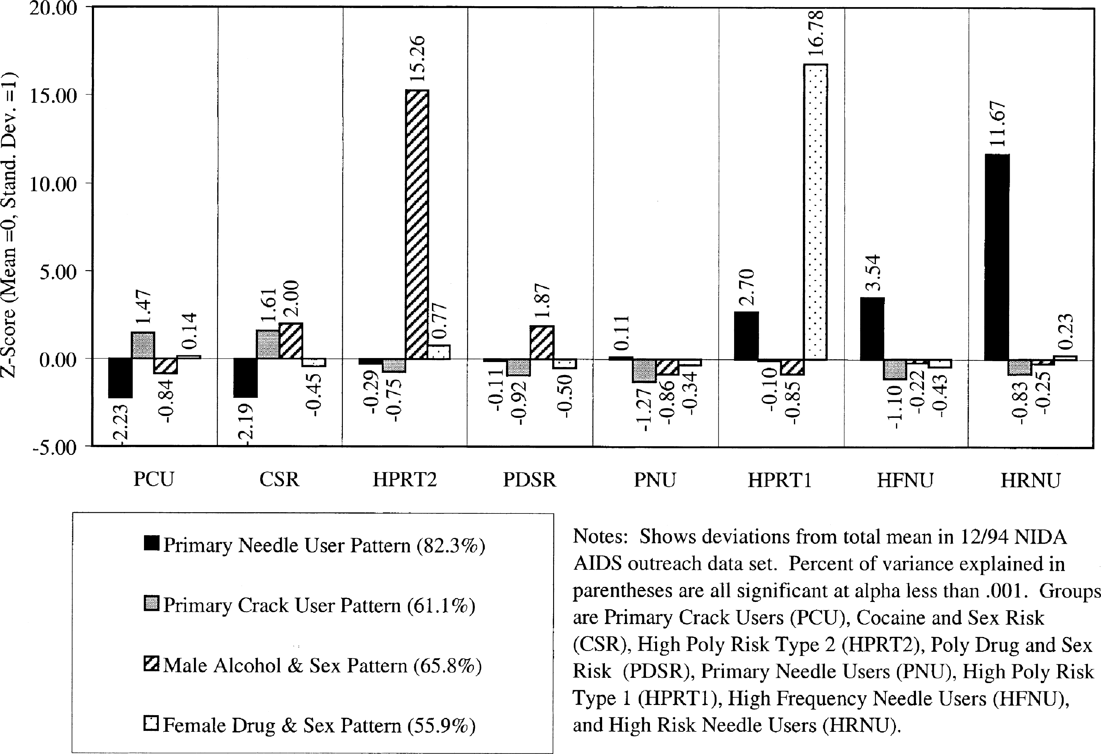
Location of clusters in four dimensions of HIV risk behaviors.
Fig. 2 compares these subgroups of drug users in terms of their rates of HIV testing and sero-prevalence. Overall 10% tested positive for HIV, and 15% went untested. The sero-prevalence rates varied significantly (, P < 0.0001) from 6 to 9% for the non-to-low frequency needle using groups, up to 15–18% in the higher frequency needle using groups, and 24% in high risk (needle sharing) group. By way of comparison, the United Nations AIDS Information Centre and World Health Organization (1998) estimates that at the end of 1997 there were approximately 810,000 adults (aged 15–49) living with HIV or AIDS in the US—or the equivalent of a sero-prevalence rate of 0.8%. This is less than 1/12th the overall rate in our out-of-treatment drug users (including the largely ‘non-needle using’ primary crack user subgroup) and less than 1/30th the rate found in the needle sharers. While it would be commonplace to collapse the three smallest groups into their nearest neighbor, from a program planning and policy perspective, it is important to note that two of these small groups have the first (HRNU) and third (HPRT1) highest rates of HIV sero-prevalence and two have the first (HPRT2) and second (HPRT1) highest rates of being ‘untested’. Thus, while work may have to be more qualitative with these smaller groups, they may represent a very promising rate of return in managing the total risk of this population.
Fig. 2.
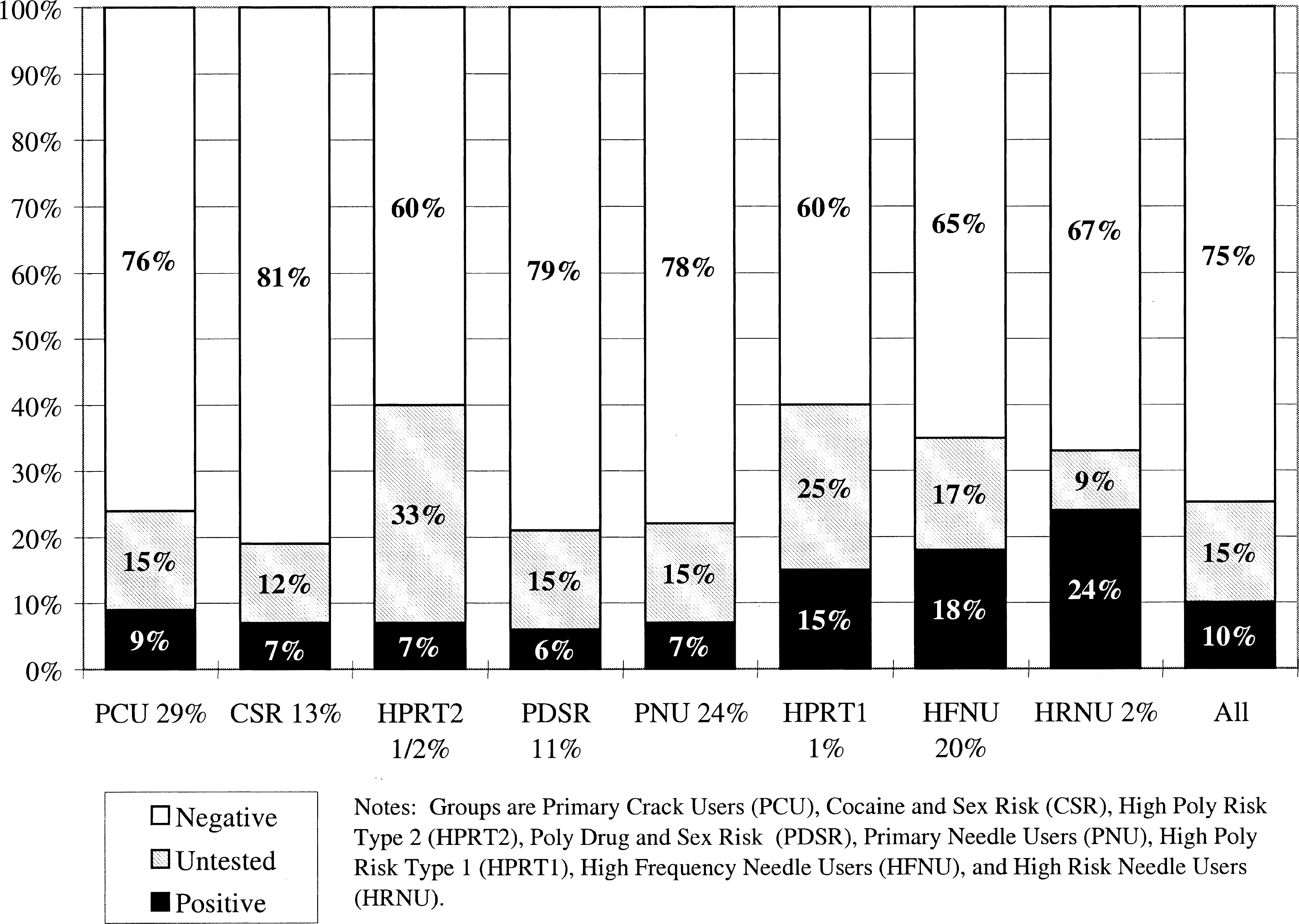
HIV status by risk group.
The risk groups were also significantly related (P < 0.0001) to demographics (gender, race, age, education), major status variables (marital, housing, employment, and criminal justice status) and simple risk factors (needle use history, substance use pattern, sexual partners, current sexual activity) as well as the 20 conceptual measures of HIV risk behaviors. Figs. 3–6 profile the eight risk groups of drug users in terms of the original 20 indices related to substance use, needle use, sexual activity, and multi-risk behaviors. Like Fig. 1, they show the deviation of each group from total mean expressed as a z-score (mean of 0, standard deviation of 1). Recall that the direction of positive scales (e.g. cleaning needles, using protection during sex, risk reduction) were all reversed so that higher numbers always mean higher risk and lower numbers always mean lower risk. The percentage of variance explained in a scale by the risk group variable is presented after the name of each scale. Again, all are significant, with the probability of Type 1 error being less than 0.0001. This is largely an artifact of the large sample size and they actually vary considerably in terms of the percentage of variance explained by the subgroups (discussed more under ‘validation’ later). Below are brief descriptions of each of the eight subgroups, including a discussion of these profiles.
Fig. 3.
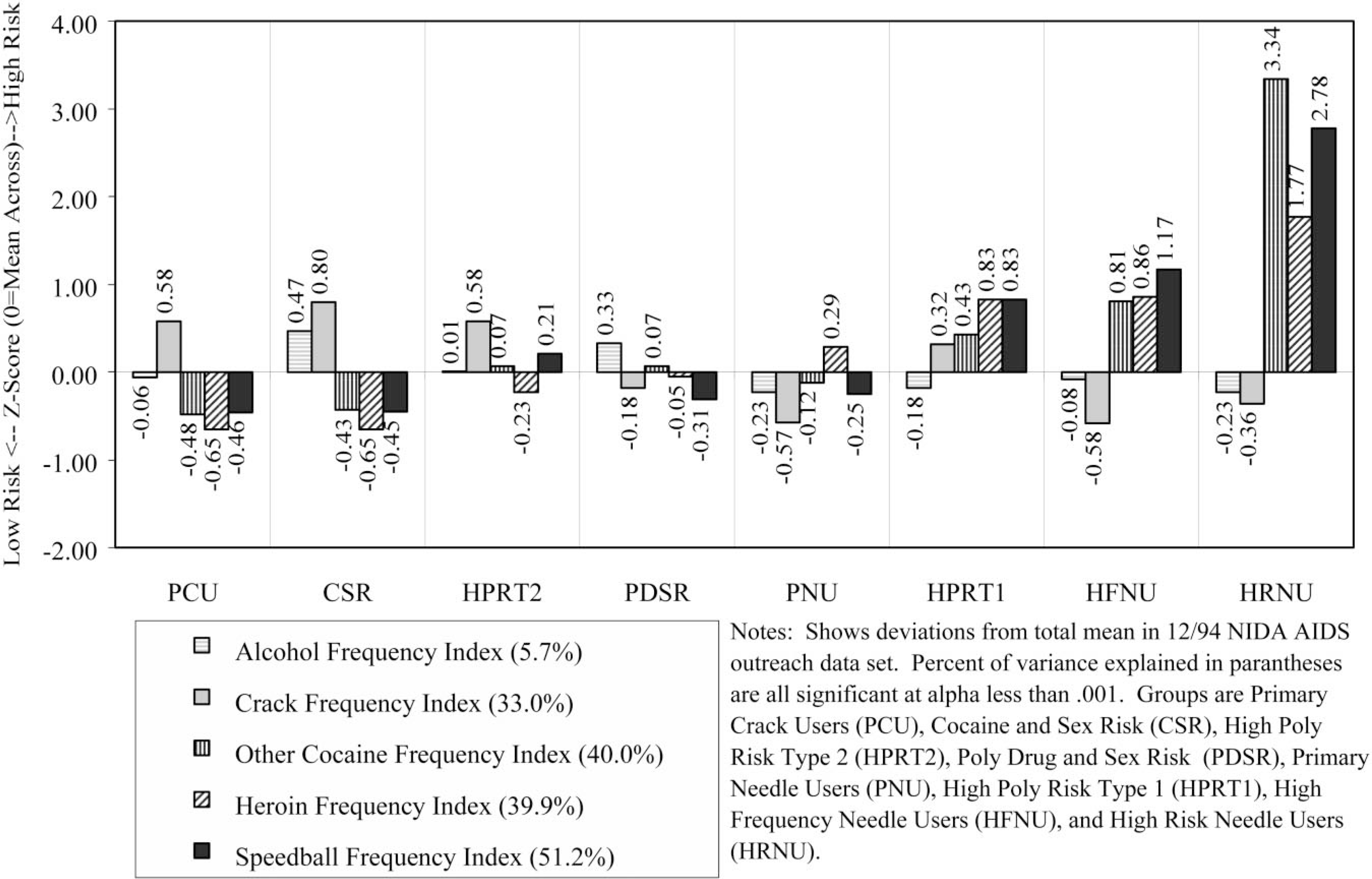
Substance use profile.
Fig. 6.
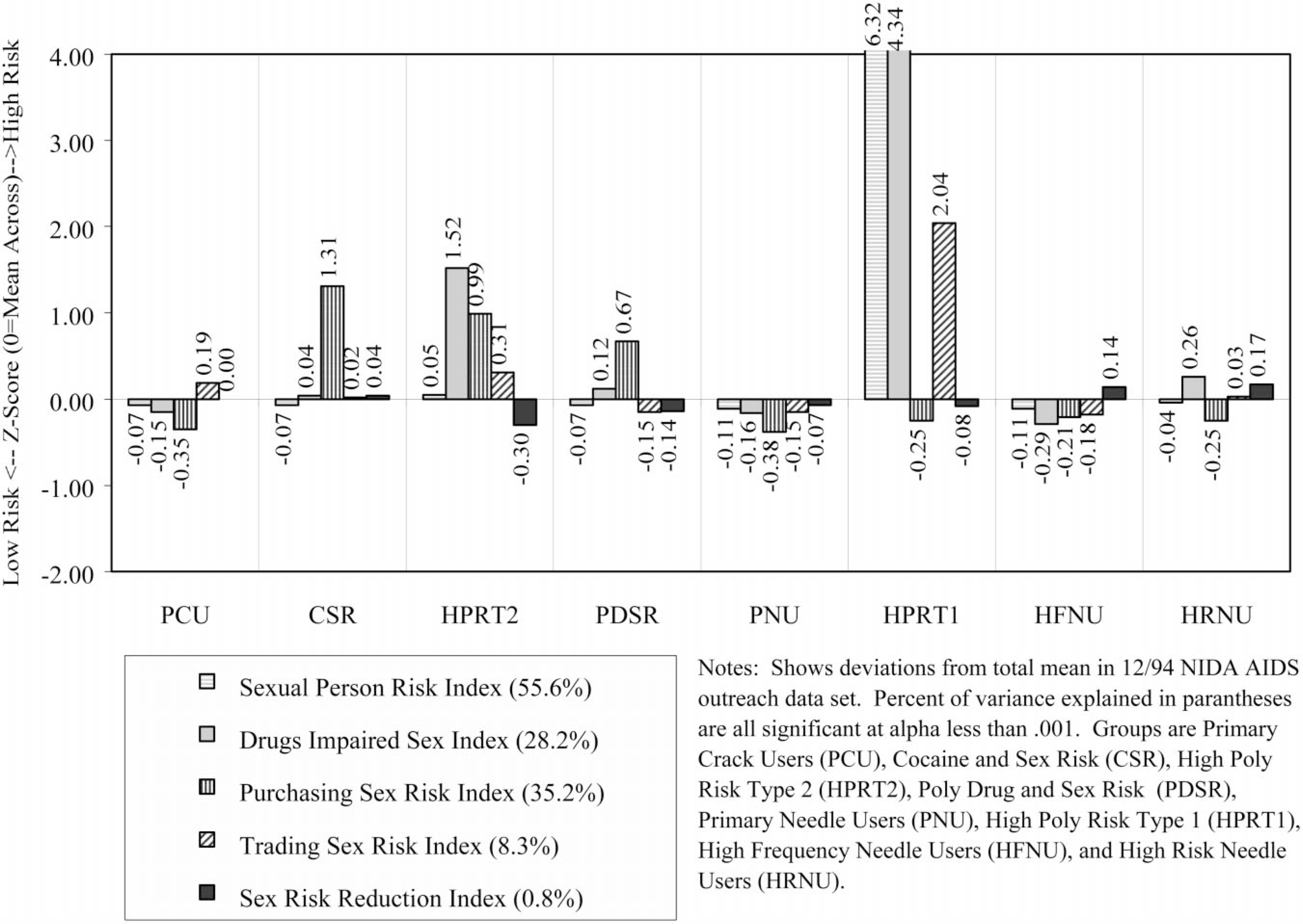
Multi-risk behavior profile.
4.2. Risk group profiles
4.2.1. Primary crack/cocaine users (29.2% PCU)
Demographically, this group was disproportionately female (52% female), predominately Black (71%), likely to be single (51%), and largely 25 years of age or older (89%). During the previous month, 30% had been homeless, 19% employed, and 7% arrested. Only 15% reported any lifetime needle use, with 9% reporting use in the past month. During the past 30 days, 96% reported using crack, 49% had a single sexual partner, 25% had multiple sexual partners, and 1% were men who had sex with men. As noted above, 9% were seropositive for HIV and 15% were untested. In terms of the substance use profile (Fig. 3), this group has an average rate of alcohol use, is tied for the second highest frequency of crack use, and is tied with CSR for the lowest rates of using cocaine, heroin, or speedballs. The high risk for failure to clean needles or change needle-related behaviors (Fig. 4) is a methods artifact, as they do not ‘need’ to do these things since they do not use needles. Rates of sexual activity (Fig. 5) are close to average, with males at particularly low risk because of condom use and/or celibacy. Rates of multi-risk behaviors (Fig. 6) for this group suggest average to lower than average risk.
Fig. 4.
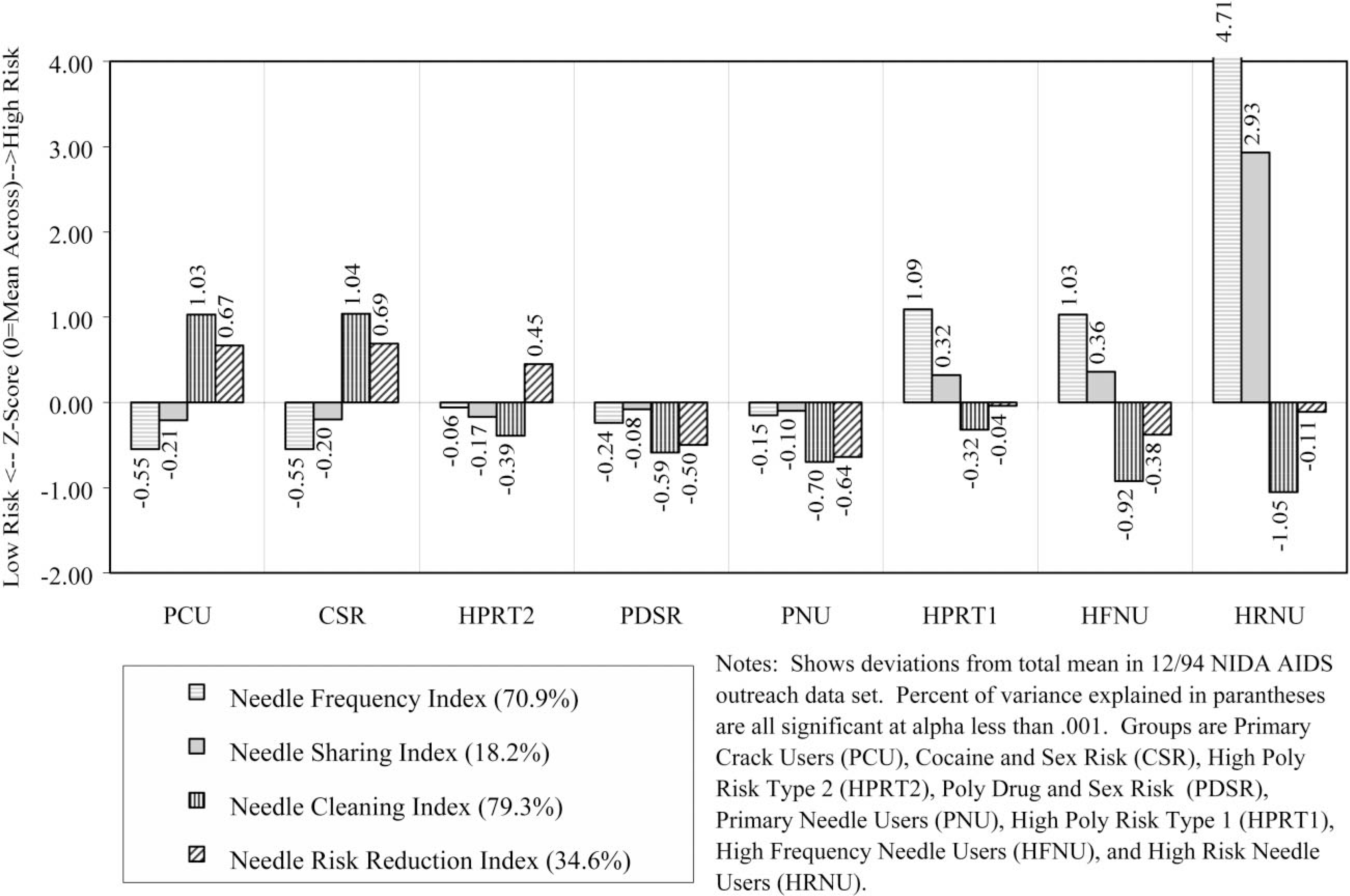
Needle use profile.
Fig. 5.
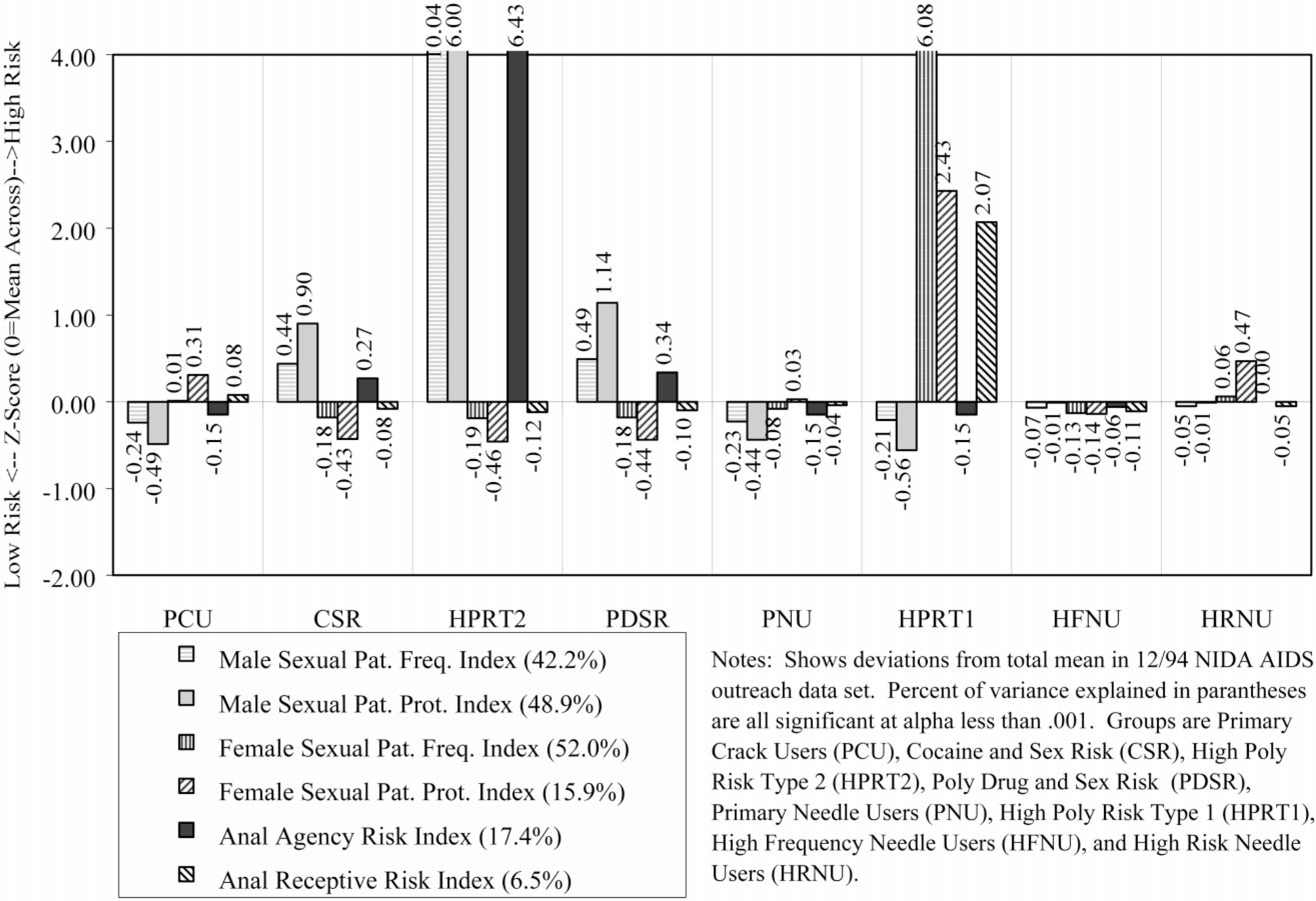
Sexual activity profile.
4.2.2. Cocaine and sexual risk (12.8% CSR)
Demographically, this group was virtually all male (99%), predominately Black (79%), the most likely to be single (52%), and largely 25 years of age or older (94%). During the prior month, 42% had been homeless, 28% employed, and 7% arrested. About 18% reported any lifetime needle use, with only 8% reporting use in the past month. During the past 30 days, 97% reported using crack, 39% had a single partner, 61% had multiple sexual partners, and 4% were men who had sex with men. As noted above, 7% were seropositive for HIV and 12% were untested. In terms of the substance use profile (Fig. 3), this group has the highest rates of alcohol and crack use, and is tied with PCU for the lowest rates of using cocaine, heroin, or speedballs. Like PCU, the high risk for failure to clean needles or change needle-related behaviors (Fig. 4) is a methods artifact as they do not ‘need’ to do these things since they do not use needles. Rates of male pattern sexual activity (Fig. 5) are the third highest in terms of both frequency, failure to use condoms, and being the agent in anal sex. Rates of multi-risk behaviors (Fig. 6) in this group are actually relatively average except for the fact that they are the group most likely to purchase sex with drugs or money.
4.2.3. High poly risk type 2 (0.3% HPRT2)
Demographically, this group was all male (100%), predominately Hispanic (47%) or Black (27%), the most likely to be separated, divorced, or widowed (53%), and it also included the largest percent of people under age 25 (20%). During the previous month, 47% had been homeless, 27% employed, and 0% reported being arrested. Over 47% reported lifetime needle use, with 49% reporting needle use in the past month. During the past 30 days, 64% reported using crack, 13% had a single partner, 87% had multiple sexual partners, and 0% were men who had sex with men. As noted above, 7% were seropositive for HIV and 33% were untested (the highest of any group). In terms of the substance use profile (Fig. 3), this group had average alcohol use, was tied with PCU for the second-highest rate of crack use, and had close to ‘average’ rates of using cocaine, heroin, or speedballs. This group did appear to clean needles but had not made many attempts to change their pattern of needle use (Fig. 4). Rates of male pattern sexual activity (Fig. 5) are the highest in terms of both frequency, failure to use condoms, and being the agent in anal sex. Rates of multi-risk behaviors (Fig. 6) in this group are the second highest for drug impaired sex and purchasing sex with drugs or money.
4.2.4. Poly drug and sexual risk (10.9% PDSR)
Demographically, this group was almost entirely male (99%), proportionately Black (60%), proportionately single (45%), and largely older than age 25 (95%). During the previous month, 32% had been homeless, 26% employed, and 9% arrested. Over 99% reported lifetime needle use, with 97% reporting needle use in the past month. During the past 30 days, 49% reported using crack, 51% had a single partner, 49% had multiple sexual partners, and 3% were men who had sex with men. As noted above, 6% were seropositive for HIV and 15% were untested. In terms of the substance use profile (Fig. 3), this group had the second highest rate of alcohol use, average rates of using crack, heroin, and other forms of cocaine and below-average rates of using speedballs. This group had below average needle use, did largely clean their needles and had attempted to change their needle use patterns (Fig. 4). Rates of male pattern sexual activity (Fig. 5) were the second highest in terms of both frequency, failure to use condoms, and being the agent in anal sex. Rates of multi-risk behaviors (Fig. 6) in this group are the third highest for purchasing sex with drugs or money but otherwise average.
4.2.5. Primary needle users (24.1% PNU)
Demographically, this group was proportionately male (67%), slightly less likely to be Black (48%), single (42%), and largely 25 years of age or older (96%). During the previous month, 29% had been homeless, 17% employed, and 8% arrested. Virtually all (99%) admitted to lifetime needle use and 97% reporting using needles in the past month. (This group did include some non-injecting opioid users.) During the previous 30 days, 30% reported using crack, 47% had a single partner, 14% had multiple sexual partners, and 1% were men who had sex with men. As noted above, 7% were seropositive for HIV and 15% were untested. In terms of the substance use profile (Fig. 3), this group was tied for the lowest alcohol use and reported the second lowest rate of crack use, average rates of other cocaine use, above average heroin use (including heroin smokers), and below average speedball use. This group had average rates of needle use and appeared to be reducing their risk by cleaning their needles or attempting to change their patterns of needle use (Fig. 4). Rates of female pattern sexual activity (Fig. 5) were below average risk; rates of male pattern sexual activity and anal sex were average. Rates of multi-risk behaviors (Fig. 6) were below average for purchasing sex but otherwise average.
4.2.6. High poly risk type 1 (1.3% HPRT1)
Demographically, this group was overwhelmingly female (95%), less likely to be Black (36%), disproportionately Hispanic (33%), proportionately single (44%), and included a sizeable group of people under age 25 years (18%). During the previous month, 49% had been homeless (the highest), 8% employed (tied for the lowest), and 21% arrested (the highest). Most (89%) reported lifetime needle use and 72% reporting using needles in the past month. During the past 30 days, 57% reported using crack, 3% had a single partner, 97% had multiple sexual partners (the highest), and 5% were men who had sex with men (all of the men in this group). De facto, this group was made up of people trading sex for drugs and to a lesser extent money. As noted above, 15% were seropositive for HIV (third highest) and 25% were untested (second highest). In terms of the substance use profile (Fig. 3), this group had average alcohol use, above average crack use, and the third highest rates of using cocaine, heroin, and speedballs. This group had the second highest rate of needle use, third highest rate of sharing, was attempting to clean their needles, and was average in attempting to reduce their risk by changing their patterns of needle use (Fig. 4). Rates of female pattern sexual activity (Fig. 5) were more than 6 standard deviations above any other group; moreover, the rates of having unprotected sex and being the receptive partner in anal sex were 2 standard deviations above any other group. Rates of multi-risk behaviors (Fig. 6) were the highest by 2–4 standard deviations for having multiple partners/IDU partners, drug-impaired sex, and trading sex to get drugs or money.
4.2.7. High frequency needle users (19.8% HFNU)
Demographically, this group was proportionately male (77%), less likely to be Black (38%) or single (37%), and largely older than 25 years of age (97%). During the previous month, 30% had been homeless, 12% employed, and 7% arrested. All (100%) reported lifetime needle use, with 99% reporting needle use in the past month. During the past 30 days, 22% reported using crack, 47% had a single partner, 22% had multiple sexual partners, and 0.5% were men who had sex with men. As noted above, 18% were seropositive for HIV (second highest) and 17% were untested. In terms of the substance use profile (Fig. 3), this group had average alcohol use, the lowest crack use, and the second highest rates of using other forms of cocaine, heroin, and speedballs. This group had the third highest rate of needle use, second highest rate of sharing, and was attempting to reduce their risk through cleaning needles and/or changing their patterns of needle use (Fig. 4). Rates of sexual activity (Fig. 5) were all average. The rates of drug-impaired sex (Fig. 6) were slightly below average, but the other multi-risk behaviors were average.
4.2.8. High risk needle users (1.6% HRNU)
Demographically, this group was proportionately male (68%), the most likely to be Hispanic (65%), second most likely to be separated, divorced or widowed (49%), and was about 12% under age 25. During the previous month, 33% had been homeless, 9% employed, and 13% arrested (second highest). All (100%) reported lifetime needle use with 99% reporting needle use in the past month. During the previous 30 days, 59% reported using crack, 33% had a single partner, 33% had multiple sexual partners, and 1% were men who had sex with men. As noted above, 24% were seropositive for HIV (highest) and 9% were untested (lowest). In terms of the substance use profile (Fig. 3), this group had below average alcohol and crack use and the highest rates of using other forms of cocaine, heroin, and speedballs. This group had the highest rate of needle use and sharing by over 2 standard deviations, but was attempting to clean needles and had made an average number of attempts to change their patterns of needle use (Fig. 4). Rates of sexual activity (Fig. 5) were average except for a higher-than-average rate of females failing to use condoms. The rates of multi-risk behaviors (Fig. 6) were slightly above average in terms of drug-impaired sex and slightly below average for trading sex to get drugs or money.
4.3. Community differences
Methodologically, the preceding profiles suggest that there is considerable risk for specification error or potentially spurious correlations when using what might otherwise seem like relatively straightforward variables. For instance, 98% of the female drug abusers are in one of four groups (PCU, PNU, HFNU, HPRT1) and two groups are less than 1% female (CSR, HPRT2). Here, we would like to focus on the issue of combining or comparing results across different communities. For multi-site analyses, many researchers would try to put in a dummy variable for site to control for community differences. The problem with this approach, as illustrated in Fig. 7, is that the site or ‘community’ is almost completely confounded with our HIV risk subgroups. Since our risk group variable is collinear with both site and virtually all of the potential measures of change in the RBA (discussed further below), including a ‘dummy’ site variable prevents almost any other clinically relevant variable from being entered into many analyses. Conversely, failure to control for the substantial differences in risk groups between sites might render multi-site comparisons fairly meaningless (e.g. if a specific intervention only works for crack users, the success rate in a given site would largely be an artifact of the percent of subjects in that site who were crack users).
Fig. 7.

Comparisons of HIV risk subgroups by site and overall.
There are some important alternative approaches to this issue. First, we can use the risk group variable to compare sites within given risk groups (e.g. how well did each do with a similar type of client). Second, we can use statistical models, such as hierarchical linear models. Third, we can use the case mix in Fig. 7 to help classify sites that are similar to each other in terms of who they are serving. In this case, we would group them into three main population patterns.
Miami, St Louis, Anchorage, Lexington, and Flagstaff, which are dominated by largely non-needle using crack groups (PCU, CSR) or the mixed groups (HPRT2, PDSR).
New York, New Orleans, Denver, Philadelphia, Houston, Long Beach, Columbus-Dayton, Puerto Rico, and Detroit, each of which has a substantial mix of both non-needle and needle using groups.
Portland, Hartford, DC, Tucson and San Francisco, which are dominated by the needle using groups (PNU, HPRT1, HFNU, HRNU).
Comparisons within each of these three groups are going be less confounded with case mix differences than those across the three groups. Moreover, we have been able to apply the group variable to the newer sites that were not included in the original sample (Dennis et al., 1998) and draw some conclusions that Rio de Janeiro, Brazil, and Durham/Wake, clearly fall in the first group, while San Antonio falls in the third.
4.4. Validation
The fundamental purpose of developing a risk group typology would be to help with program planning and evaluation. By clustering on the major dependent variables that can be used to measure change, we are basically creating a multivariate pre-test. Unlike simple pretests that only address the main effects of a single baseline behavior, our risk group typology also takes into account the interactions. But how well does this work? Below are brief summaries of several analyses we have done to evaluate this cluster solution of HIV risk groups.
4.4.1. Reverse validation
To assess the model fit of a given cluster solution, Rapkin and Luke (1993) recommend that the cluster variable be used in a multiple analysis of variance (MANOVA) to predict the variables from which it was derived—a test they referred to as ‘reverse validation’. Fig. 1 on the four factor dimensions and Figs. 3–6 on the 20 conceptual measures show the differences between each group: next to the label for each scale is the percentage of variance explained in that scale by the ‘Risk Groups’. The graphed values are z-scores and show the difference from the grand mean of the total sample (0) to the centroid of each subgroup divided by the number of standard deviations for that score. This is a form of an ‘effect size’. Thus, a score of about 0.2 is a small difference, 0.4 a moderate difference, 0.8 or larger a major difference. The observed differences range from −2.23 to +16.78 and reveal a very heterogeneous population. At baseline, these HIV Risk Groups of drug users were able to explain 55.9–82.3% of the variance in the four statistical dimensions and 99.6% of their joint distribution. For the 20 conceptual indices it explained from 0.0 to 79.3% and 99.9% of their joint distribution, this includes 50% or more for the variance of five measures, 30–49% for the variance of seven, 10–29% of the variance of four, and 0–10% for four (alcohol frequency, anal receptive anal risk, trading sex risk, and sex risk reduction). The high percentage of variance explained in the joint distribution can be interpreted as a good model fit (i.e. reverse validation) and minimizes the need for additional covariates unless one is just looking at a handful of the measures (Rapkin & Luke, 1993).
4.4.2. Predictive validity
In terms of evaluation, one of the most important tests of our risk group typology is the extent to which it can be used as a blocking or stratifying variable when predicting the future. Though the NIDA cooperative agreement studies were still collecting data in the field at the time these data were created (and still are at this writing), we had access to follow-up RBFAs for 1799 drug users (~40%). The risk group variable was significantly related to the probability of completing a follow-up interview (, P < 0.0001). Moreover, three of the four lowest rates of follow-up were in the groups with above average rates of HIV (HPRT1, HFNU, HRNU), and the fourth had the highest rate of being untested (HPRT2).
Using the baseline risk group, we were able to explain from 12.8 to 36.4% of the variance in the four statistical dimensions, 62.8% of their joint distribution at follow-up, 0.3–37.2% of the variance of the 20 conceptual indices, and 77.1% of their joint distribution.
This means that our risk group measure can be used as a multidimensional covariate or blocking variable and dramatically increase power or reduce the required sample size. For a given level of power (80%) and Type 1 error (0.05), using the risk group measure would reduce the sample size required to detect a given effect size of:
0.01 from 1569 to 199 people;
0.35 from 274 to 35 people;
0.50 from 68 to 10 people (Dennis, Lennox & Foss, 1997).
More important, however, is the fact that these risk groups help bring the impact of interventions into focus. To illustrate this, we calculated the effect size of the pre- to-post change in each of the 21 simple questions overall and then within each of the eight risk groups. Then, we classified the effects by direction (increased or decreased risk) and by effect sizes (according to one widely used convention (Cohen, 1988; Lipsey, 1990). Effect sizes can be interpreted as: no effect if 0 to 0.19, small if 0.2–0.39, medium if 40–0.79, and large if 0.80 or more (Dennis et al., 1997 for a discussion of effect sizes). Out of the 21 measures evaluated across groups, 12 showed no effect, eight showed a small reduction in risk behaviors, and one showed a small increase in risk behaviors. However, because effect sizes vary by subgroup, the average effect size is likely to be misleading and may vary largely as a function of the case mix ( i.e. driven by the effectiveness of the largest subgroups in a given sample). The ‘within individual risk groups’ comparisons showed an average of five no effects, eight small decreases in risk behaviors, four medium decreases, two large decreases, and two small increases in risk behaviors. The difference between these results occurred because many of the large effects were limited to the relevant group (e.g. reduced needle sharing among needle sharers, reduced trading sex among the small groups of women who were actively trading sex). Averaging these effects over other people washed them out. Fig. 8 also shows that the number of ‘no effects’ ranged from a high of 18 of the 21 questions evaluated to a low of three.
Fig. 8.

Range of effect sizes for 21 questions by HIV risk group.
4.4.3. Comparison with alternative adjustments
To evaluate how well the risk groups work at explaining risk behaviors, Table 2 compares how well our expected risk group did at predicting the variance of the four main dimensions at baseline and follow-up relative to (a) site dummy variables, (b) gender, (c) NIDAs prior target population variable (Injector, crack user or both), and (d) current sexual activity. At baseline it did better than all of the other models. At follow-up it did better on every measure than all the models except for ‘target population’, which did slightly better at predicting the crack user dimensions (37.6 vs. 36.4%).
Table 2.
Percentage of variance explained at baseline and follow-up by alternative models for predicting risk
| Criterion Variables | [Variable] | Individual risk group (Initial)a |
||||
|---|---|---|---|---|---|---|
| Sitea [PSITE] | Gender [GENDER] |
Target populationb [TARPOP] |
Current sexual patternc [CSEXPAT] |
Baseline expected risk groupd [ERG8] |
||
|
| ||||||
| Risk Behavior Assessment (RBA)e | ||||||
| Primary Needle User Pattern Dimension | [PNUPD_6F] | 19.9† | 0.3* | 41.0† | 3.3† | 82.3† |
| Primary Crack User Pattern Dimension | [PCUPD_4F] | 20.4† | l.3† | 53.4† | l.9† | 61.1† |
| Male Alcohol and Sex Pattern Dimension | [MASPD_5F] | 2.6† | 13.9† | 1.0† | 28.2† | 65.8† |
| Female Drug and Sex Pattern Dimension | [FDSPD_6F] | 1.4† | 15.l† | 0.4* | 27.6† | 55.9† |
| Joint Distribution (1-Lambda) | 46.51 | 29.4† | 64.2† | 50.3† | 99.6† | |
| Risk Behavior Follow-up Assessment (RBFA)f | ||||||
| Primary Needle User Pattern Dimension | [PNUPD_6F] | 10.7† | 0.1nsd | 21.2† | 0.4nsd | 31.0† |
| Primary Crack User Pattern Dimension | [PCUPD_4F] | 23.7† | 1.0† | 37.6† | 2.1† | 36.4† |
| Male Alcohol and Sex Pattern Dimension | [MASPD_5F] | 2.7† | 9.0† | 0.9* | 12.l† | 12.8† |
| Female Drug and Sex Pattern Dimension | [FDSPD_6F] | 1 –5† | 16.1† | 0.2nsd | 20.4† | 19.5† |
| Joint Distribution (1-Lambda) | 31.3† | 25.7† | 42.7† | 32.6† | 62.8† | |
| Degrees of Freedom Required by the Model | 18 | 1 | 2 | 5 | 7 | |
Anchorage, Columbus-Dayton, Denver, Detroit, Flagstaff, Hartford, Houston, Lexington, Long Beach, Miami, New Orleans, New York, Philadelphia, Portland, Puerto Rico, San Francisco, St Louis, Tucson, Washington, DC.
Injection Drug User, Crack User, or Both.
Celibate, Male Heterosexual, Male Bisexual, Male Homosexual, Female Heterosexual, Female Bisexual, Female Lesbian.
Primary Crack Users (PCU), Crack and Sexual Risk (CSR), High Poly Risk Type 1 (HPRT1), Poly Drug and Sexual Risk (PDSR), Primary Needle Users (PNU), High Poly Risk Type 2 (HPRT2), High Frequency Needle Users (HFNU), High Risk Needle Users (HRNU).
Observed at Month = 0, with n = 4445.
Observed at Month = 6, with n = 1799
(nsd no significant difference, *P < 0.001, †P < 0.0001). Source: NIDA AIDS Cooperative Agreement Q1 Methodology Study Data Set (25% of 12/94 Data Set)
4.4.4. Cross validation and replication
We also wanted to be able to prospectively classify future individual respondents on a case-by-case basis for cross-site analyses and even for prospective blocking ( i.e. stratification) prior to randomization. All of the alphas and percents of variance predicted were within a tenth of a percentage point when we ran them on the second random quarter of the national data. This result is not really surprising since, with such large sample sizes, this comparison turns into a test of ‘random sampling’ and the ‘law of large numbers’ to average things out. We, therefore, replicated the analysis again on a third sample from our North Carolina site that had not been in the original data. Note that, despite the small sample size, the North Carolina sample included all eight subgroups (as did nearly every other site in the original analysis). This time it actually did better in terms of the observed alpha and percentage of variance it was able to predict in the future. The latter factor may result because North Carolina follow-ups were being completed an average of one month earlier than in the older national data set. We also look at the ability of the discriminant rule based on only 21 items to predict the group. Despite the fact that it was based on 1/10th of the variables, the percent of variance predicted at intake and follow-up was never off by more than one percentage point.
4.4.5. Checking for potential regression to the mean
One of the questions that repeatedly comes up discussing these results is whether they might simply be the result of regression to the mean (Campbell & Stanley, 1963; Cook & Campbell, 1979). This happens when people are initially selected based on extreme scores on a pretest score (or a closely related measure) and then changes are measured in this score (or the related measure). We do not believe this happened here for several reasons. First, the thresholds for inclusion (dirty urine from any use or needle tracks) were very low relative to those used in treatment studies (e.g. dependence and averages of weekly or daily use). If any lower, people would be out of the target population to whom the study was designed to generalize. Second, many of the variables that did change (e.g. frequency of alcohol use, sexual protection, trading sex for drugs) were not part of the inclusion/exclusion criteria but showed the same pattern. The reader may wonder whether the risk groups differences are due to regression to the mean. If this were so, then the low groups should go up and the high groups go down. Yet here, all groups go down; in fact, a quick review of Fig. 8 shows that the ratio of positive to negative effect sizes ranged from 2:1 to 13:0.
5. Implications and next steps
Like most multivariate methods, cluster analysis is highly dependent on what is included in the model and is often open to multiple interpretations. Our approach here was to focus on the measures of change that could be used in arguably the largest multi-site study of AIDS outreach to drug users in the US, Puerto Rico, and Brazil. Our assumption was that, if things like gender or homelessness were going to be correlated with a risk behavior at follow-up, they would probably also be correlated with that behavior at baseline. By clustering on the dependent variables at baseline, we believe that we have constructed a multivariate pretest that combines main effects and several interactions. While this may be somewhat more difficult to interpret, we believe that it is actually a more accurate representation of the answers given by out-of-treatment drug users (who had nothing near factorially distributed risk behaviors).
From a program planning point of view, we have tried to demonstrate that, while a focus on needle use is important, it is not sufficient. While 60% of the drug users in this study had used needles, most did so infrequently, and were trying to clean or change their pattern of use: 76% did not share needles. Interventions should acknowledge the steps they have taken but check on their effectiveness. If they recognize and use information on early attempts to change, outreach workers may also be able to help motivate drug users to enter more formal substance abuse treatment.
The big news for program planning, however, is the complicated mosaic of relationships between drugs and sex. The three male groups purchasing sex for drugs or money (CSR, HPRT2, and PDSR) and the one female group selling sex for drugs or money (HPRT1) are coming in contact with many people, and they may need very different interventions than the other groups that were dominated by people who had been with 0–1 sexual partner in the past month. Moreover, it is not clear that these four high-risk groups even need the same things. For instance, the HPRT2 and HPRT1 also had significantly higher elevations of using drugs during sex, whereas the other two seemed not to be doing so.
Further investigation of primary crack users is needed. Neither their needle use nor sexual practices offer a simple explanation as to why their rates of HIV are so high and are comparable with primary needle users. Anecdotal evidence suggests that it may be related to increased genital abrasions that result from prolonged intercourse and/or their ignoring pain or the lack of lubrication. However, this is just speculation and needs to be confirmed qualitatively.
Methodologically, this paper also helped to demonstrate the heterogeneity of community-based samples and the importance of subgroup analysis for increasing design sensitivity and interpretation. We have already used this risk group variable as a blocking variable before randomization took place in our Durham/Wake site to facilitate other cross-site analyses (Wechsberg et al., 1998). We also continue to explore other potentially simpler ways of controlling for these real differences among out-of-treatment drug users. Our current work is aimed at the development of simpler classification rules based on a few variables in this data set that would capture most of the critical variation in the eight groups and could be used in other studies.
Acknowledgements
This research was supported by Cooperative Agreement No. U01 DA08007 from the National Institute on Drug Abuse (NIDA). The opinions expressed are solely those of the authors and do not reflect official positions of NIDA. This research was undertaken in response to several methodological problems raised by the NIDA and cooperative agreement staff over the past several years and builds heavily on their earlier works. In addition to their advice, this entire study would not have been possible without the use of data pooled across the all of the contributing sites. We are deeply indebted to the principal investigators of the individual sites for sharing their data, staff from NIDA, NOVA, Inc., and several sites working on methodological issues, and the feedback several individuals. To list only some, they include: Marcia Anderson, Robert Booth, Linda Cottler, Susan Coyle, Sherry Deren, David Desmond, Dennis Fisher, Jeffrey Hoffman, James Inciardi, Lynne Kotranski, Carl Leukefeld, Clyde McCoy, Isaac Montoya, Richard Needle, Fen Rhodes, Rafaela Robles, Vernon Shorty, Harvey Siegal, Merrill Singer, Joe Sonnefeld, Michael Stark, Sally Stevens, Robert Trotter, John Watters, Norman Weatherby, and Mark Williams. We would also like to thank Theresa Gurley, Bruce MacDonald, Rebecca Perritt, Nat Rodman, and Joan Unsicker for their assistance in preparing this manuscript. We are deeply indebted to Joe Sonnefeld and Robert Orwin for detailed reviews.
Appendix
Fisher’s Linear Discriminant Functions Classification Coefficients Used in Simplified Scale (Will be available at www.chestnut.org/li/posters/erq8disc.pdf or from first author)
| Variable | Discriminant Function Coefficients For Each ERG8 Group |
|||||||
|---|---|---|---|---|---|---|---|---|
| PCU | CSR | HPRT2 | PDSR | PNU | HPRT1 | HFNU | HRNU | |
| (Constant) | −9.5256811 | −14.2354952 | −107.6834213 | −23.9992212 | −22.1523119 | −92.0019890 | −28.7661984 | −58.2098691 |
| ABDYIJD E_Q11c(2)D Days cocaine inject,30days | −0.0167314 | −0.0508543 | −0.0611582 | 0.0155422 | 0.0373515 | 0.1517761 | 0.1971307 | 0.4986981 |
| ABDYIJE E_Q11c(2)E Days heroin inject,30days | 0.0116773 | 0.0135438 | 0.0261488 | 0.0244880 | 0.0693353 | 0.1914762 | 0.1727936 | 0.2433349 |
| ABDYIJF E_Q11c(2)F Days speedball inject,30days | −0.0126573 | 0.0011325 | 0.1044831 | 0.0167040 | 0.0247315 | 0.2181187 | 0.3157803 | 0.4763756 |
| ACTIJ30 E_Q12 Times injected drugs Iast30days | −0.0010523 | 0.0011298 | −0.0021240 | −0.0022537 | −0.0040802 | 0.0159642 | 0.0173840 | 0.0726617 |
| ACTUSED E_Q13a Times know used works used,30days | 0.0126154 | 0.0130732 | 0.0092146 | 0.0305794 | 0.0321655 | 0.0446481 | 0.0512644 | 0.1339841 |
| DCTOW30 Times reused own works (30 days) | 1.0604183 | 0.6499748 | 1.5912349 | 9.6545387 | 10.6243217 | 9.7571089 | 10.7821165 | 10.2263333 |
| ABDYLSTC E_Q11c(1)C Days used crack,30days | 0.1454098 | 0.1541702 | 0.1065052 | 0.0802779 | 0.0501068 | 0.1087166 | 0.0564465 | 0.0917287 |
| DCNSW30 # new works used (30 days) | 1.2426918 | 1.2065855 | 6.2934652 | 14.9218451 | 14.7965543 | 11.2982872 | 13.4820601 | 11.9478459 |
| AHRISKC E_Q76a-C Cleaned needles with bleach | −0.2706532 | −0.6026369 | 0.0085517 | 1.6470681 | 2.7048649 | 1.1739651 | 2.7265570 | 2.9856181 |
| AHRISKF E_Q76a-F Other change in sexual patterns | 0.5657241 | 0.3557716 | 0.7587281 | 1.3505697 | 1.2305001 | 2.1226581 | 1.1160563 | 1.6708755 |
| ABDYLSTA E_Q11c(1)A Days used alcohol,30days | 0.0752217 | 0.0992712 | 0.0086143 | 0.1132084 | 0.0836163 | 0.0596288 | 0.1025394 | 0.0930018 |
| DGEGDHST Q60a Given Drugs for Sex (30 days) | −0.9537802 | 6.7853522 | 12.3069080 | 4.8898304 | −0.8241450 | −1.9443025 | 0.2448226 | −0.2130950 |
| VAG_A Vaginal Sex Agency Frequency | 0.0987901 | 0.2346209 | 1.1739707 | 0.2263290 | 0.0711337 | 0.0457593 | 0.0866663 | 0.0605612 |
| VAG_APR Vaginal Sex Agency Protection | 7.0019701 | 5.1781147 | 12.3656640 | 5.2405423 | 7.1327368 | 6.6789699 | 6.0508261 | 5.6026158 |
| ANA_A Anal Sex Agency Frequency | −0.0239295 | 0.4187242 | 6.4717658 | 0.2289126 | −0.2470253 | −0.5935229 | −0.3341066 | −0.5121560 |
| AFSEXP E_Q26 # of different people had sex with | −0.0163367 | −0.0211577 | −0.0906294 | −0.0175450 | −0.0194834 | 0.6941934 | −0.0386776 | −0.0685959 |
| AFTDDSC E_Q58-C Times used crack w/ sex | −0.0272316 | −0.0098714 | 0.3234193 | −0.0042885 | 0.0042722 | −0.0176920 | 0.0126183 | 0.0234946 |
| DGEGSGDT Q59a Give Sex to Get Drugs (30 days) | 1.2280306 | 0.0977336 | −3.5023939 | −0.4094149 | 0.0743621 | 4.1204153 | −0.2524749 | −0.5232699 |
| VAG_R Vaginal Sex Reception Frequency | 0.1016081 | 0.0881481 | 0.0240879 | 0.1254822 | 0.1277311 | 0.5666543 | 0.1442765 | 0.1898007 |
| VAG_RPR Vaginal Sex Reception Protection | 9.3239297 | 10.5729857 | 8.8112935 | 10.9127429 | 10.5104164 | 15.5200120 | 11.0075956 | 11.7893287 |
| ANA_R Anal Sex Reception Frequency | 0.2670791 | 0.1950068 | −0.1570425 | 0.1000703 | 0.0574662 | 3.2282755 | −0.0320661 | −0.0480036 |
References
- Aldenderfer MS, & Blashfield RK (1984). Cluster analysis, Newbury Park, CA: Sage Publications. [Google Scholar]
- Anderberg M (1973). Cluster analysis for applications, New York, NY: Academic Press. [Google Scholar]
- Anderson M, Hockman E, & Smereck GAD (1996). Effect of a nursing outreach intervention to drug users in Detroit, Michigan. Journal of Drug Issues, 26 (3), 619–634. [Google Scholar]
- Anderson RN, Kochanek KD, & Murphy SL (1997). Report of final mortality statistics, 1995. Monthly Vital Statistics Report, l45(11), (Supp. 2, Table 7). Hyattsville, MD: National Center for Health Statistics. www.cdc.gov/nchswww/SSBR/45112t07.htm [Google Scholar]
- Association of State and Territorial Health Officers (ASTHO) (1988). Intravenous drug use and HIV transmission: recommendations by the ASTHO Committee on HIV, Washington, DC: ASTHO. [Google Scholar]
- Ben-Abdallah A, Cottler LB, Compton WM, Dinwiddie SH, & Woodson SM (1996). Subtyping Risks of HIV Infection: A Latent Class Analysis of Drug and Sex Behaviors. Presentation at the American Psychological Association Conference, Toronto, Canada. [Google Scholar]
- Blattner WA, Biggar RJ, Wiess SH, Melbye M, & Goedert JJ (1985). Epidemiology of human T-lymphotropic virus type III and the risk of acquired immunodeficiency syndrome. Annals of Internal Medicine, 103, 665–670. [DOI] [PubMed] [Google Scholar]
- Booth R, Crowley TJ, & Zhang Y (1996). Substance abuse treatment entry, retention, and effectiveness: Out-of-treatment opiate injection drug users. Drug and Alcohol Dependence, 42, 11–20. [DOI] [PubMed] [Google Scholar]
- Brown B, Beschner G, & The National AIDS Consortium. (1993). At risk for AIDS: Injection drug users and sexual partners, Westport, CT: Greenwood Press. [Google Scholar]
- Campbell DT, & Stanley JS (1963). Experimental and quasi-experimental designs for research on teaching. In Gage NL, Handbook of research on teaching. Boston: Houghton Mifflin Co. [Google Scholar]
- Carlson RG, Wang J, Siegal HA, Falck RS, & Guo J (1994). An ethnographic approach to targeted sampling: Problems and solutions in AIDS prevention research among injection drug and crack cocaine users. Human Organization, 53, 279–286. [Google Scholar]
- Centers for Disease Control (1987). HIV virus in the US: a review of current knowledge. MMWR, 36(Supp. 6), 52–53. [Google Scholar]
- Centers for Disease Control (1995). HIV/AIDS prevention, Atlanta, GA: Centers for Disease Control. [Google Scholar]
- Centers for Disease Control (1996). HIV/AIDS Surveillance Report, 8(1). Atlanta, GA: Author. [Google Scholar]
- Centers for Disease Control and Prevention. (1997). HIV/AIDS Surveillance Report, 9(2). Atlanta, GA: Author. [Google Scholar]
- Cohen J (1988). Statistical power analysis for the behavioral sciences, Hillsdale, NJ: Lawrence Erlbaum Associates. [Google Scholar]
- Colon H, Sahai H, Robles RR, & Matos TD (1995). Effects of a community outreach program in HIV risk behaviors among injection drug users in San Juan, Puerto Rico: An analysis of trends. AIDSS Education and Prevention, 7 (3), 195–209. [PubMed] [Google Scholar]
- Cook TD, & Campbell D (1979). Quasi-experimentation: Design and analysis issues for field settings, Boston, MA: Houghton-Mifflin. [Google Scholar]
- Coyle S (1993). The NIDA standard intervention model for injection drug users not in treatment: Intervention manual, Rockville, MD: National Institute on Drug Abuse. [Google Scholar]
- Coyle SL, Boruch RF, & Turner CF (Eds.). (1989). Evaluating AIDS prevention programs. Washington, DC: National Academy Press. [PubMed] [Google Scholar]
- Dennis ML & Wechsberg WM (1996). Methodological lessons from the NIDA AIDS outreach program. Paper presented at the American Psychological Association Meeting, Toronto, Ontario, Canada. [Google Scholar]
- Dennis ML, Lennox RD, & Foss MA (1997). Practical power analysis for planning substance abuse prevention and services research. In Bryant KJ, Windle M & West SG, Recent advances in prevention research methodology: Lessons from alcohol and substance abuse research. Washington, DC: American Psychological Association. [Google Scholar]
- Dennis ML, McDermeit M, & Wechsberg WM (1998). Overview of the NIDA new cohort cross-site meta analysis. Presentation at the American Public Health Association conference, Washington, DC, November 17. [Google Scholar]
- Deren S, Davis WR, Beardsley M, Tortu S, & Clatts M (1995). Outcomes of a risk reduction intervention with high risk populations: The Harlem AIDS Project. AIDS Education and Prevention, 7 (5), 379–390. [PubMed] [Google Scholar]
- Des Jarlais DC, & Friedman SR (1987). HIV infection among intravenous drug users: Epidemiology and risk reduction. AIDS, 1 (1), 67–76. [PubMed] [Google Scholar]
- Dowling-Guyer S, Johnson ME, Fisher DG, Needle R, Watters J, Anderson M, Williams M, Kotranski L, Booth R, Rhodes F, Wearthby N, Estrada AL, Fleming D, Deren S, & Tortu S (1994). Reliability of drug users’ self-reported HIV risk behaviors and validity of self-reported recent drug use. Assessment, 1, 383–392. [Google Scholar]
- Dwyer R, Richardson D, Ross MW, Wodak A, Miller ME, & Gold J (1994). A comparison of HIV risk between women and men who inject drugs. AIDS Education and Prevention, 6 (5), 379–389. [PubMed] [Google Scholar]
- Friedland GH, Harris C, Butkus-Small C, Shine D, Moll B, Darrow W, & Klein R (1985). Intravenous drug users and the Acquired Immunodeficiency Syndrome: Demographics, drug users and needle sharing patterns. Archives of Internal Medicine, 145, 1413–1417. [PubMed] [Google Scholar]
- Gerstein DR, Ingles J, Datta R, Talley K, Jordan K, Schildhaus S, Johnson R, Rasinski K, Taylor J, Bacellar H, Anderson D, Phillips D, Collins J, Condelli W, Ciftan E, & Rohde F (1997). National Treatment Improvement Evaluation Study (NTIES) Main Findings. Rockville, MD: SAMHSA Center for Substance Abuse Treatment. [Google Scholar]
- Haverkos HW, & Lange WR (1990). Serious infections other than immunodeficiency virus among intravenous drug abusers. Journal of Infectious Diseases, 161, 894–902. [DOI] [PubMed] [Google Scholar]
- Higgins DL, Galavotti C, O’Reilly KR, Schuell DJ, Moore M, Rug DL, & Johnson R (1991). Evidence for the effects of HIV antibody counseling and testing on risk behaviors. Journal of the American Medical Association, 266 (17), 2419–2429. [PubMed] [Google Scholar]
- Illinois Department of Public Health, AIDS Activity Section (1997). Special runs provided from state data. Author. [Google Scholar]
- Inciardi J (1994). HIV/AIDS risks among male, heterosexual non-injecting drug users. In NIDA Research Monograph Series: The Context of HIV Risks Among Drug Users and Their Sexual Partners. Rockville, MD: National Institute on Drug Abuse. [Google Scholar]
- Joe GW, & Simpson DD (1995). HIV risks, gender, and cocaine use among opiate users. Drug and Alcohol Dependence, 37, 23–28. [DOI] [PubMed] [Google Scholar]
- Jose B, Friedman SR, Neaigus A, Curtis R, Grund JPC, Goldstein MF, Ward TP, & Des Jarlais DC (1993). Syringe-mediated drug-sharing (backloading): A new risk factor for HIV among injection drug users. AIDS, 7, 1653–1660. [DOI] [PubMed] [Google Scholar]
- Koester SK (1994). Copping, running, and paraphernalia laws: Contextual variables and needle risk behavior among injection drug users in Denver. Human Organization, 53 (3), 287–295. [Google Scholar]
- Koester SK, Booth R, & Wiebel W (1990). The risk of HIV transmission from sharing water, drug mixing containers and cotton filters among intravenous drug users. International Journal of Drug Policy, 1 (6), 28–30. [Google Scholar]
- Kraemer HC (1992). Evaluating medical tests: Objective and quantitative guidelines, Newbury Park, CA: Sage. [Google Scholar]
- Leukefeld CG, Battjes RJ, & Amsel RJ (1990). AIDS and intravenous drug use: Community intervention and prevention, New York: Hemisphere Publishing. [Google Scholar]
- Lipsey MW (1990). Design sensitivity: Statistical power for experimental research, Newbury Park, CA: Sage. [Google Scholar]
- Little R, & Rubin DB (1989). The analysis of social science data with missing values. Sociological Methods and Research, 18 (2), 292326. [Google Scholar]
- Longshore D, & Anglin MD (1995). Number of sex partners and crack cocaine use: Is crack an independent marker for HIV risk behavior? Journal of Drug Issues, 22 (1), 1–16. [Google Scholar]
- McCoy CB, & Inciardi JA (1995). Sex, drugs, and the continuing spread of AIDS, Los Angeles, CA: Roxbury Publishing. [Google Scholar]
- McCoy CB, Weatherby NL, Metsch LR, McCoy HV, Rivers JE, & Correa R (1996). Effectiveness of HIV interventions among crack users. Drugs and Society, 7, 137–154. [Google Scholar]
- Needle RH & Coyle SL (1997). Community based outreach risk reduction strategy to prevent HIV risk behaviors in out-of-treatment injection drug users, (NIH Consensus Development Conference on Interventions to Prevent HIV Risk Behaviors). Rockville, MD: National Institute on Drug Abuse, Division of Epidemiology and Prevention Research, Community Research Branch. [Available from first author at RN28E@nih.gov.] [Google Scholar]
- Office of Applied Studies (OAS) (1997). Preliminary results from the 1996 National Household Survey on Drug Abuse. Rockville, MD: Substance Abuse and Mental Health Services Administration, Office of Applied Studies. [Google Scholar]
- Oliver KJ, Friedman SR, Maynard H, Magnuson L, & Des Jarlais DC (1992). Impact of a needle exchange program on potentially infectious syringes in public places. Journal of Acquired Immune Deficiency Syndromes, 5 (5), 534–535. [DOI] [PubMed] [Google Scholar]
- Rapkin BD, & Luke DA (1993). Cluster analysis in community research: Epistemology and practice. American Journal of Community Psychology, 21, 247277. [Google Scholar]
- Rhodes F, & Malotte CK (1996). HIV risk interventions for active drug users: Experience and prospects. In Oskamp S & Thompson SC, Understanding and preventing HIV risk behaviors (pp. 207–236). Thousand Oaks, CA: Sage. [Google Scholar]
- Sechrest L, McNight P, & McNight K (1996). Calibration of measures for psychotherapy outcome studies. American Psychologist, 51 (10), 1065–1071. [DOI] [PubMed] [Google Scholar]
- Shrout PE, Spitzer RL, & Fleiss JL (1987). Quantification of agreement in psychiatric diagnosis revisited. Archives of General Psychiatry, 44, 172–177. [DOI] [PubMed] [Google Scholar]
- Stall R, & Leigh B (1994). Understanding the relationship between drug or alcohol use and high risk sexual activity for HIV transmission: Where do we go from here? Addiction, 89, 131–134. [DOI] [PubMed] [Google Scholar]
- Stephens Simpson, Coyle McCoy, & The NADR Consortium. (1993). Comparative effectiveness of NADR interventions. In Brown BS & Beschner GM, Handbook on risk of AIDS (pp. 519–556). Westport, CT: Greenwood Press. [Google Scholar]
- Stevens SJ, Tortu S, & Coyle SL (Eds.) (1998). Women, drug use and HIV infection. New York, NY: Haworth Medical Press. [Google Scholar]
- Stryker J & Smith MD (Eds.) (1993). Dimensions of HIV prevention: Needle exchange. Menlo Park, CA: Kaiser Forums. [Google Scholar]
- Trotter RT, Bowen AM, Baldwin JA, & Price LJ (1996). The efficacy of network based HIV/AIDS risk reduction programs in mid sized towns in the United States. Journal of Drug Issues, 26 (3), 591–605. [Google Scholar]
- Turner CF, Miller HG, & Moses LE (Eds.) (1989). AIDS: Sexual behavior and intravenous drug use. Washington, DC: National Academy Press. [PubMed] [Google Scholar]
- United Nations AIDS Information Centre and World Health Organization (UNAIDS/WHO, 1998). Report on the global HIV/AIDS Epidemic June 1998. Page 66. Geneva, Switzerland: UNAIDS Information Centre. [Google Scholar]
- US Department of Health and Human Services (1994). Outreach/risk reduction strategies for changing HIV-related risk behaviors among injection drug users. (NIH Publication No. 94–3726). Rockville, MD: Author. [Google Scholar]
- Ward J (1963). Hierarchical grouping to optimize an objective function. Journal of the American Statistical Association, 58, 236–244. [Google Scholar]
- Watkins JD, Conway-Welch C, Creedon JJ, Crenshaw TL, DeVos RM, Gebbie KM, Lee BJ III, Lilly F, O’Connor JC, Primm BJ, Pullen P, SerVaas C, & Walsh WB (1988). Report of the Presidential Commission on the human immunodeficiency virus epidemic (Submitted to the President of the United States). Washington, DC: US Government Printing Office. [PubMed] [Google Scholar]
- Watters JK, & Biernacki P (1989). Targeted sampling: Options for the study of hidden populations. Social Problems, 36, 416–430. [Google Scholar]
- Weatherby NL, Needle R, Cesari H, Booth R, McCoy C, Watters J, Williams M, & Chitwood D (1994a). Validity of self-reported drug use among injection drug users and crack cocaine users recruited through street outreach. In Dennis ML & Wechsberg WM (Eds.), Special issue: Evaluating drug abuse interventions. Evaluation and Program Planning, 17, 347–355. [Google Scholar]
- Weatherby NL, Needle R, Cesari H, Booth R, McCoy C, Watters J, Williams M, & Chitwood D (1994b). Reply to Wish and Mieczkowski. In Dennis ML & Wechsberg WM (Eds.), Evaluating drug abuse interventions. Evaluation and Program Planning, 17, 331–342. [Google Scholar]
- Wechsberg WM & Cavanaugh ER (1998). Differences found between women in and out of treatment. In Stevens S and Wexler H (Eds.), Drugs and Society, 13(12), 65–82. [Google Scholar]
- Wechsberg WM, Dennis ML, & Ying Z (1995). Women and men injectors: Differences and trends in their drug use patterns and HIV risk. Presentation at the meeting of the American Public Health Association, San Diego, CA. [Google Scholar]
- Wechsberg WM, Dennis ML, & Stevens SJ (1998). Cluster analysis of HIV intervention outcomes among substance abusing women. The American Journal of Drug and Alcohol Abuse, 24 (2), 239–257. [DOI] [PubMed] [Google Scholar]
- Wechsberg WM, Stevens SJ, Rasch RFR, Dennis ML, Rodman N, & Estrada A (1997). Regional and gender Differences in drug and sexual patterns, HIV risk, and behavioral changes with ethnic diversity. Presentation at the College on Problems on Drug Dependency (CPDD), Nashville, TN. [Google Scholar]
- Weeks MR, Himmelgreen DA, Singer M, Wolley S, Romero-Daza N, & Grier M (1996). Community based AIDS prevention: Preliminary outcomes of a program for African American and Latino Injection Drug Users. Journal of Drug Issues, 26, 561–590. [Google Scholar]
- Wiebel WW, Jimenez A, Johnson W, Ouellet L, & Jovanovic B (1996). Risk behavior and HIV sero-incidence among out-of-treatment injection drug users: A four year prospective study. Journal of Acquired Immune Deficiency, 12, 282–289. [DOI] [PubMed] [Google Scholar]
- Williams ML, Zhao Z, Freeman RC, Elwood WN, Rusek R, Booth RE, Dennis ML, Fisher DG, & Rhodes F (1998). A cluster analysis of not-in-treatment drug users at risk for HIV infection. The American Journal of Drug and Alcohol Abuse, 24 (2), 199–223. [DOI] [PubMed] [Google Scholar]