Noise2Void: Unsupervised Denoising of PET Images

Abstract

Elevated noise levels in positron emission tomography (PET) images lower image quality and quantitative accuracy and are a confounding factor for clinical interpretation. Recent advances in deep learning have ushered in a wide array of novel denoising techniques, several of which have been successfully adapted for PET image reconstruction and post-processing. The bulk of the deep learning research so far has focused on supervised learning schemes, which, for the image denoising problem, require paired noisy and noiseless/low-noise images. This requirement tends to limit the utility of these methods for medical applications as paired training datasets are not always available. Furthermore, to achieve the best-case performance of these methods, it is essential that the datasets for training and subsequent real-world application have consistent image characteristics (e.g., noise, resolution, etc.), which is rarely the case for clinical data. To circumvent these challenges, it is critical to develop unsupervised techniques that obviate the need for paired training data. In this paper, we have adapted Noise2Void, a technique that relies on corrupt images alone for model training, for PET image denoising and assessed its performance using PET neuroimaging data. Noise2Void is an unsupervised approach that uses a blind-spot network design. It requires only a single noisy image as its input, and, therefore, is well-suited for clinical settings. During the training phase, a single noisy PET image serves as both the input and the target. Here we present a modified version of Noise2Void based on a transfer learning paradigm that involves group-level pretraining followed by individual fine-tuning. Furthermore, we investigate the impact of incorporating an anatomical image as a second input to the network. We validated our denoising technique using simulation data based on the BrainWeb digital phantom. We show that Noise2Void with pretraining and/or anatomical guidance leads to higher peak signal-to-noise ratios than traditional denoising schemes such as Gaussian filtering, anatomically guided non-local means filtering, and block-matching and 4D filtering. We used the Noise2Noise denoising technique as an additional benchmark. For clinical validation, we applied this method to human brain imaging datasets. The clinical findings were consistent with the simulation results confirming the translational value of Noise2Void as a denoising tool.

1. Introduction

Positron emission tomography (PET) is an in vivo molecular imaging technique that enables 3D visualization of radiotracers which bind to specific molecular targets with functional or physiological significance. PET has emerged as a vital player in clinical settings for deep-tissue mapping of cellular metabolism, neuroreceptor density, pathological protein aggregation, etc. with applications spanning oncology, neurology, cardiology, and beyond (Farwell et al. 2014, Delbeke et al. 1999, Salmon et al. 2015, Farde et al. 1989, Bergmann et al. 1984). Accurate interpretation of PET images is of high clinical significance both in the context of diagnostics and therapeutic assessment. Elevated noise levels in PET images, however, pose a challenge to accurate quantitation and adversely impact clinical workflows. Specific protocol-related contributors to PET noise include radiotracer dose reduction (which can limit a patient’s radiation exposure) and scan time reduction (possibly to limit patient discomfort or increase throughput). Both tracer dose and scan time reduction could lead to reconstructed images with reduced photon counts and, hence, higher noise levels. The reconstruction of low-count PET images is usually followed by a post-filtering step for denoising. Typically, clinical workflows rely on simple Gaussian filters that smooth over the local neighborhood of each voxel. While convenient to use, the Gaussian filter is not edge-preserving and leads to spillover of intensities across different regions-of-interest (ROIs). To date, a broad range of edge-preserving and/or non-local filters have been applied to PET images. Efforts geared toward preserving edges in PET images include anisotropic smoothing techniques like the bilateral filter (Hofheinz et al. 2011), wavelet-based techniques (Lin et al. 2001), and spatiotemporal smoothing techniques designed for dynamic PET images (Tauber et al. 2011, Christian et al. 2010, El Fakhri et al. 2005). The non-local means (NLM) filter (Buades et al. 2005), which was demonstrated to outperform traditional edge-preserving approaches, has been successfully applied to PET imaging (Dutta, Leahy & Li 2013). Block-matching and 3D (BM3D) filtering (Dabov et al. 2007) and its higher dimensional variants BM4D and BM5D have also been applied to PET imaging (Ote et al. 2020). A number of newer techniques use innovative strategies to incorporate high-resolution anatomical information into existing denoising frameworks. In particular, the performance of wavelet denoisers (Boussion et al. 2009, Le Pogam et al. 2013) and NLM filters (Chan et al. 2014, Arabi and Zaidi 2020) have been improved by the incorporation of anatomical information. Guided filtering (He et al. 2013), another approach that integrates cross-modality information, has also been used for PET image denoising (Yan et al. 2015).

Over the last several years, the image processing and computer vision community has witnessed the emergence of a broad range of novel denoising techniques that exploit recent advances in deep learning. Several of these methods have been adapted for the PET image denoising and low-dose image reconstruction tasks. Neural networks used to denoise PET images include those with simpler architectures, such as basic convolutional neural networks (CNNs) (Gong et al. 2019, da Costa-Luis and Reader 2021), as well as those with more sophisticated architectures like encoder-decoder setups (Chen et al. 2020, Xu et al. 2017), U-Net (Liu and Qi 2019, Schaefferkoetter et al. 2020), or generative adversarial networks (Wang et al. 2018, Zhou et al. 2020). However, the majority of existing deep learning based denoising approaches are supervised learning techniques, which require paired training data, i.e., corrupt input and clear target image pairs for network training. In addition, despite their high best-case accuracy in one dataset, the generalizabilty of these approaches rests on the consistency of image characteristics across datasets. These constraints have generated a strong interest in unsupervised denoising techniques for PET (Cui et al. 2019). The Noise2Noise (N2N) technique, which relies on two or more input noise realizations and obviates the need for high-count ground truth images, partially addresses the challenges associated with supervised learning (Lehtinen et al. 2018). This technique has been adapted for PET image denoising (Chan et al. 2019, Yie et al. 2020), but its utility is limited by the additional constraint it poses in that it requires more than one noise realization. Very recently, a new technique known as Noise2Void (N2V) has been developed, which does not require paired training samples or multiple noise realizations (Krull et al. 2019). In this paper, we present an adaptation of N2V denoising for PET neuroimaging and assess the performance of this approach using simulation and clinical studies. We show here that N2V denoising performance can be enhanced by transfer learning (via group-level, simulation-based pretraining) and the incorporation of anatomical information. In section 2, we describe the network architecture, the simulation and clinical datasets, and strategies for network training, validation, and group-level pretraining. In section 3, we present simulation and clinical results evaluating the performance of the N2V denoising framework and comparing it with alternative denoising techniques. In section 4, we discuss this approach and highlight its benefits and limitations. Finally, we summarize our results in section 5.

2. Methods

2.1. Network Architecture

The N2V approach is based on network training using input and target images that are identical and noisy. In this setting, a conventional network would generate a prediction that is identical to the input. N2V, however, uses a blind-spot network design as illustrated in Figure 1. A blind-spot network applies a mask on each input patch that excludes the central pixel. Whereas a network with a regular receptive field and the noisy image patch set as both the input and the training target would output a replica of the noisy input, a blind-spot masking scheme that excludes the central pixel of the input encourages a blind-spot network to seek information from neighboring pixels and use this information to learn to remove noise.

Figure 1. The blind spot concept.

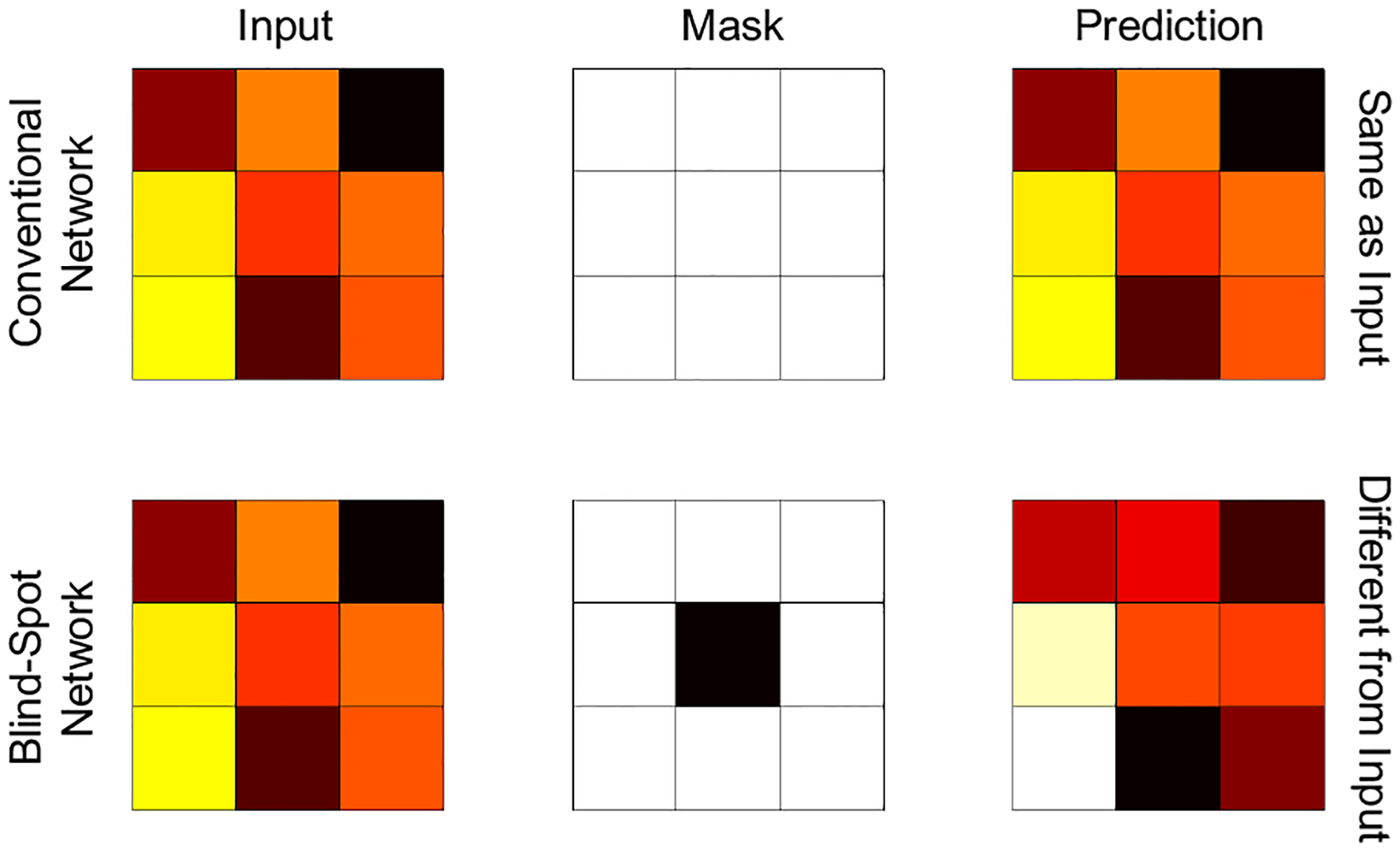
Unlike a conventional network, a blind-spot network has a masked receptive field that excludes the central pixel and can learn to suppress noise by focusing on the neighboring pixels. Thus, it can generate a prediction distinct from the input even when the input and target images are identical and noisy.

We implemented the well-known U-Net architecture (Ronneberger et al. 2015) as a blind-spot network. The network has three resolution levels. The first convolutional (conv) layer has 64 3 × 3 filters with the filter number doubling after each downsampling step, which is realized by 2 × 2 max pooling (max pool) layers. The last (output) layer has only one filter. Each convolutional layer is followed by a rectified linear unit (ReLU) activation function, except for the last layer. The stride of convolution is set to 1 with a padding of 1 pixel. The full network is shown in Figure 2.

Figure 2. Network architecture.

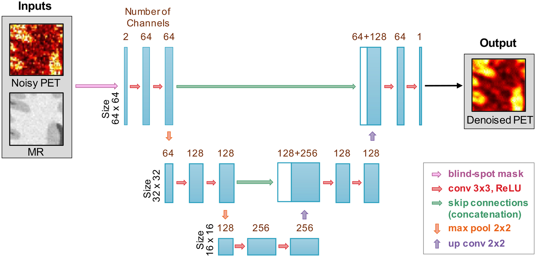
A U-Net network with a blind-spot mask applied to the input is used here for N2V denoising. Each convolutional layer is followed by a ReLU activation function, except for the last layer.

The network is trained using an L₂ loss function. For an unknown denoised PET image vectorized as $\widehat{\mathit{x}}\in {ℝ}^N$ and a target PET image (which, in this case, is the same as the input noisy image) $x_{\text{input}}\in {ℝ}^N$, where N is the number of voxels, the L₂ loss function, denoted as ${\Phi }_{\text{training}}\left(\widehat{\mathit{x}}\mid x_{\text{input}}\right)$, is computed as:

$${\Phi }_{\text{training}}\left(\widehat{\mathit{x}}\mid x_{\text{input}}\right)={\Vert \widehat{\mathit{x}}-x_{\text{input}}\Vert }_2.$$ (1)

It is not efficient to train N2V using patches where only the central pixel is excluded. To improve the method’s efficiency, 5% of the pixels in a given patch were selected to be masked out on a random basis – an idea proposed in the original N2V paper (Krull et al. 2019).

2.2. Network Inputs

Two versions of the network were implemented: one with a noisy PET image as a single-channel input and another with a multi-channel input consisting of a noisy PET image and a magnetic resonance (MR) image. The inputs consist of transverse patches of size 64 × 64 (PET only) or 64 × 64 × 2 (PET and MR input channels) extracted from the 3D image volumes. The input intensities were normalized to the intensity range [0, 1]. Data augmentation was achieved by randomly rotating the inputs by 1 to 360° and randomly cropping them to the size of 64 × 64 or 64 × 64 × 2.

2.3. Simulation Data

Realistic simulations were performed using the 3D BrainWeb digital phantom (http://brainweb.bic.mni.mcgill.ca/brainweb/). For training and validation of the N2V network, we used 3D segmented image volumes from 20 subjects derived from the BrainWeb simulated brain database. The atlases contained the following ROI labels: gray matter, white matter, and cerebrospinal fluid (CSF). PET images with a realistic gray-to-white contrast ratio of 4:1 emulating the ¹⁸F-fluorodeoxyglucose (¹⁸F-FDG) radiotracer were synthesized from the segmented volumes (Song et al. 2020b). The 3D static noiseless (ground truth) PET images had a voxel size of 1 mm × 1 mm × 1 mm with grid dimensions of 256 × 256 × 256. These “ground-truth” PET images were used for validation purposes alone as the network training is unsupervised and does not require knowledge of the true image.

The geometric model of the Siemens ECAT HR+ scanner was used to generate sinogram data. Noisy data were generated using Poisson deviates of the projected sinograms, a noise model widely accepted in the PET imaging community (Dutta, Ahn & Li 2013). The Poisson deviates were generated with mean counts of 12.5M, 25M, 50M, and 100M to test performance at different noise levels. The data were then reconstructed using the ordered subset expectation-maximization (OSEM) algorithm (12 iterations, 16 subsets). Our noisy image set consisted of OSEM-reconstructed images with no post-filtering. The N2V network uses these noisy images as both the input and target during the training phase. T1-weighted MR images derived from the BrainWeb database and downsampled to the PET resolution scale were used as additional anatomical inputs for the anatomically guided version of N2V.

2.4. Clinical Data

Clinical neuroimaging datasets used for this paper were obtained from the Alzheimer’s Disease Neuroimaging Initiative (ADNI, http://adni.loni.usc.edu/) database, a public repository containing images and clinical data from 2000+ human datasets. We selected ¹⁸F-FDG PET scans and corresponding anatomical T1-weighted MR scans for clinical validation of our method. For consistency, all datasets were based on the ADNI2 protocol. The subject details and demographics are as follows: n = 17, 10 female, age 77.41 ± 7.98 years. ¹⁸F-FDG PET data were acquired following a 5 ± 10% mCi bolus injection using a Siemens BioGraph TruePoint scanner. The scan started 30 minutes post-injection. The full scan duration was 30 minutes (6 × 5-minute frames). The OSEM algorithm (4 iterations, 14 subsets) was used for reconstruction. Our noisy image set consisted of OSEM-reconstructed images with no post-filtering. The clinical PET images had a voxel size of 1 mm × 1 mm × 2 mm with grid dimensions of 336 × 336 × 109. The image corresponding to the 3rd time-frame is used as the noisy input (and training target). There is no noiseless ground-truth image available for this clinical dataset. The mean image across the 6 time-frames was used as the reference low-noise image for validation after checking to ensure similarity of contrast levels across the 6 time-frames.

2.5. Network Training, Fine-Tuning, and Validation

The N2V network was implemented on the TensorFlow platform, and all computations were performed using an NVIDIA GTX 1080Ti graphics card. For individual validation samples, we tested two strategies. The first of these involved directly training the N2V network for individual noisy validation images. The second strategy, which is based on transfer learning, involved group-level pretraining of the network followed by fine-tuning for individual validation samples, all using noisy data alone. Validation was performed on 5 BrainWeb digital phantoms and clinical data from 10 human subjects. Separate cohorts were used for the pretraining step and the fine-tuning/validation step to ensure that the validation results are more easily generalizable to future applications involving data not encountered by the model during the pretraining step.

2D image patches of size 64 × 64 were generated from the 3D image volumes for network training/fine-tuning. The network was trained for 100 epochs. The L₂ loss function was minimized using the Adam optimizer. The learning rate was set to 0.0003, and the batch size was set to 10.

2.6. Network Pretraining

The original N2V method trains the network using identical, noisy input and target image patches. While this obviates the need for a separate “labeled” training dataset consisting of noisy and clean image pairs, it also adds a more substantial computational burden for each test/validation case. To facilitate N2V network training for individual validation samples, we introduce a group-level network pretraining strategy for N2V in this work. This pretraining step is based on the same idea of using identical noisy images as the input and the training target. But this step is performed on a separate subset of the data reserved for pretraining. Subsequently, the pretrained network is individually fine-tuned for each noisy image from the validation dataset used as both the input and the target. Both the pretraining and fine-tuning steps are unsupervised as they require noisy data samples and assume no knowledge of the ground truth.

For the BrainWeb simulations, out of the 20 digital phantoms available through the database, we used 15 noisy PET phantom images for pretraining the network model. For the human imaging studies, we used hybrid data, consisting of 15 noisy BrainWeb PET phantom images and 7 noisy human PET images for pretraining. Pretraining was based on 2D image patches generated from the 3D image volumes. Patches were created dynamically across different training epochs by randomly cropping and rotating the 3D image into 64 × 64 2D subimages.

2.7. Compared Techniques

To evaluate the proposed N2V framework, we compared the denoising performance of the Gaussian, NLM-MR, BM4D, N2N, and N2V techniques as described below. While Gaussian filtering is considered the clinical standard, NLM-MR and BM4D are recognized as reliable benchmarks for denoising in the image processing community and have therefore been included in this study. N2N, on the other hand, can be thought of as a gold-standard reference.

• Gaussian denoising: The first reference method used is conventional Gaussian filtering based on a 2D Gaussian-weighted kernel that enables averaging over the local neighborhood of a given voxel. Gaussian denoising is chosen as a reference because of its popularity and clinical prevalence for the task of post-reconstruction image smoothing. The Gaussian full at half maximum was varied over the range 2–3.75 mm to find the parameter setting that maximizes a given performance evaluation metric (peak signal-to-noise ratio).

• NLM-MR denoising: The second reference method is NLM with MR-based anatomical guidance. The NLM filter has been shown to outperform a broad range of denoising approaches, including methods that rely on local kernels as well as transform-domain methods such as wavelets. The NLM similarity metric is based on 2D spatial patches. The NLM search window size was set to 11 × 11. The patch width was varied over the range 3–7 pixels, and the filtering parameter (i.e., the standard deviation of the Gaussian weighting kernel) was varied over the range 0.25–0.6 to find the parameter setting that maximizes the evaluation metric.

• BM4D denoising: The third reference method is the BM4D filter, which is based on an enhanced sparse representation in a transform domain. The percentage of noise standard deviation for the BM4D filter was varied over the range 15–30% to find the parameter setting that maximizes the evaluation metric.

• N2N denoising: The fourth reference method is the N2N approach. For our N2N implementation, we adopted the same U-Net architecture as N2V minus the blind-spot scheme and used two noise realizations as inputs. This method is expected to exhibit stronger performance than N2V and is, therefore, more of a gold-standard reference.

• N2V denoising: The first N2V variant tested here is similar to the original N2V implementation (Krull et al. 2019). In this variant, the network training is done from scratch for individual noisy test images. There is no group-level pretraining. The noisy PET image is the sole input.

• N2V-MR denoising: The second N2V variant tested here is one where the network training is done from scratch for individual noisy test images, i.e., without group-level pretraining, and where anatomical image patches are provided as additional inputs. This method is subsequently referred to as N2V-MR.

• N2V-PT denoising: The third N2V variant tested here is one where the network is pretrained at the group level using noisy images and fine-tuned for individual images and where the noisy PET image is the sole input. This method is subsequently referred to as N2V-PT.

• N2V-PT-MR denoising: The last N2V variant tested here is one where the network is pretrained at the group level using noisy images and fine-tuned for individual images, and anatomical image patches are provided as additional inputs. This method is subsequently referred to as N2V-PT-MR.

2.8. Evaluation Metric

The primary evaluation metric used in this paper is the peak signal-to-noise ratio (PSNR). The PSNR is the ratio of the maximum signal power to noise power and is defined as:

$$\text{PSNR}(\widehat{\mathit{x}},x)=20{\text{ log}}_{10}\left(\frac{\text{max }(x)}{\text{RMSE}(\widehat{\mathit{x}},x)}\right).$$ (2)

Here the true and estimated images are denoted x and $\widehat{\mathit{x}}$ respectively, and the root-mean-square error (RMSE) is defined as:

$$\text{RMSE}(\widehat{\mathit{x}},x)=\sqrt{\frac{1}{N}\sum _k{\left({\widehat{x}}_k-x_k\right)}^2},$$ (3)

where k is the the voxel index. A second evaluation metric reported here is the structural similarity index (SSIM). The SSIM (Wang et al. 2004) is a well-accepted measure of perceived image quality and is defined as:

$$\text{SSIM}(\widehat{\mathit{x}},x)=\frac{\left(2{\mu }_x{\mu }_{\widehat{x}}+c_1\right)\left(2{\sigma }_{x\widehat{x}}+c_2\right)}{\left({\mu }_x^2+{\mu }_{\widehat{x}}^2+c_1\right)\left({\sigma }_x^2+{\sigma }_{\widehat{x}}^2+c_2\right)}.$$ (4)

Here c₁ and c₂ are parameters stabilizing the division operation. We use the notations μ_x and σ_x respectively for the mean and standard deviation of x, ${\mu }_{\widehat{x}}$ and ${\sigma }_{\widehat{x}}$ respectively for the mean and standard deviation of $\widehat{\mathit{x}}$, and ${\sigma }_{x\widehat{x}}$ for the covariance of x and $\widehat{\mathit{x}}$.

3. Results

3.1. Simulation Results

Figure 3 shows a comparison of the PSNR obtained by applying the different denoising methods to the simulation data. The PSNR was computed using the noiseless phantom images as the reference. To ensure fair comparison, we report the best value of the PSNR yielded by each method. For all noise levels, N2N has the strongest performance. This is expected since, unlike other methods, N2N uses two noise realizations. The N2V variants that use anatomical information, pretraining, or a combination of the two lead to higher mean PSNR than vanilla N2V consistently for all noise levels. Among the non-deep-learning approaches, BM4D exhibits higher PSNRs than both NLM-MR and Gaussian filtering. For the lowest noise case (100M counts), N2V-PT-MR (21.41 dB), N2V-PT (21.37 dB), N2V-MR (21.37 dB), and BM4D (21.22 dB) exhibit comparable mean PSNR performance. For this case, the mean PSNR for vanilla N2V is somewhat lower (20.92 dB) while that for NLM-MR and Gaussian is considerably lower (20.32 and 20.30 dB respectively). The margins of improvement of the N2V variants over other methods consistently increase as the noise level increases. For the highest noise case (12.5M counts), all N2V variants yield substantially higher mean PSNRs (N2V-PT-MR: 18.38 dB, N2V-PT: 18.24 dB, N2V-MR: 18.21 dB, N2V: 17.94 dB) than conventional filters (BM4D: 17.72 dB, NLM-MR: 17.64 dB, Gaussian: 17.58 dB). In summary, while N2V with pretraining and/or anatomical guidance outperforms other methods that use a single noisy PET image for all noise levels, this family of methods is the most promising for higher noise settings. Figure 4 shows a comparison of the SSIM obtained by applying the different denoising methods to the simulation data. N2V-PT-MR and N2V-MR, the two anatomically guided variants of N2V, exhibit the strongest SSIM performance relative to all other methods, including N2N. This is explained by the fact that the simulated digital phantom has a high level of consistency with the MR image.

Figure 3. PSNR comparison for the simulation data.

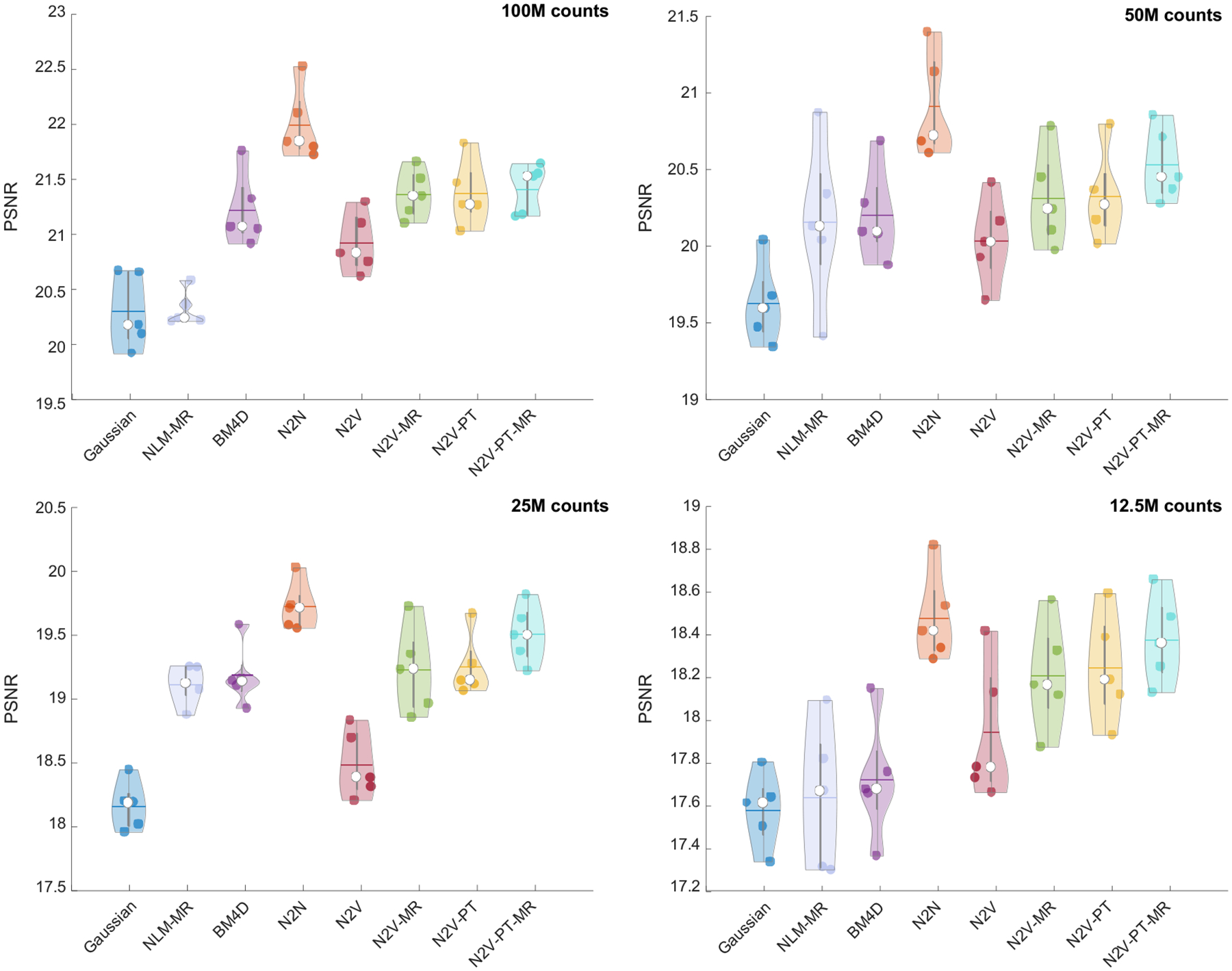
Violin plots showing the PSNR distributions for the PET images obtained using Gaussian, NLM-MR, BM4D, N2N, N2V, N2V-MR, N2V-PT, and N2V-PT-MR denoising. The results are shown for four different noise levels: 100M counts, 50M counts, 25M counts, and 12.5M counts.

Figure 4. SSIM comparison for the simulation data.

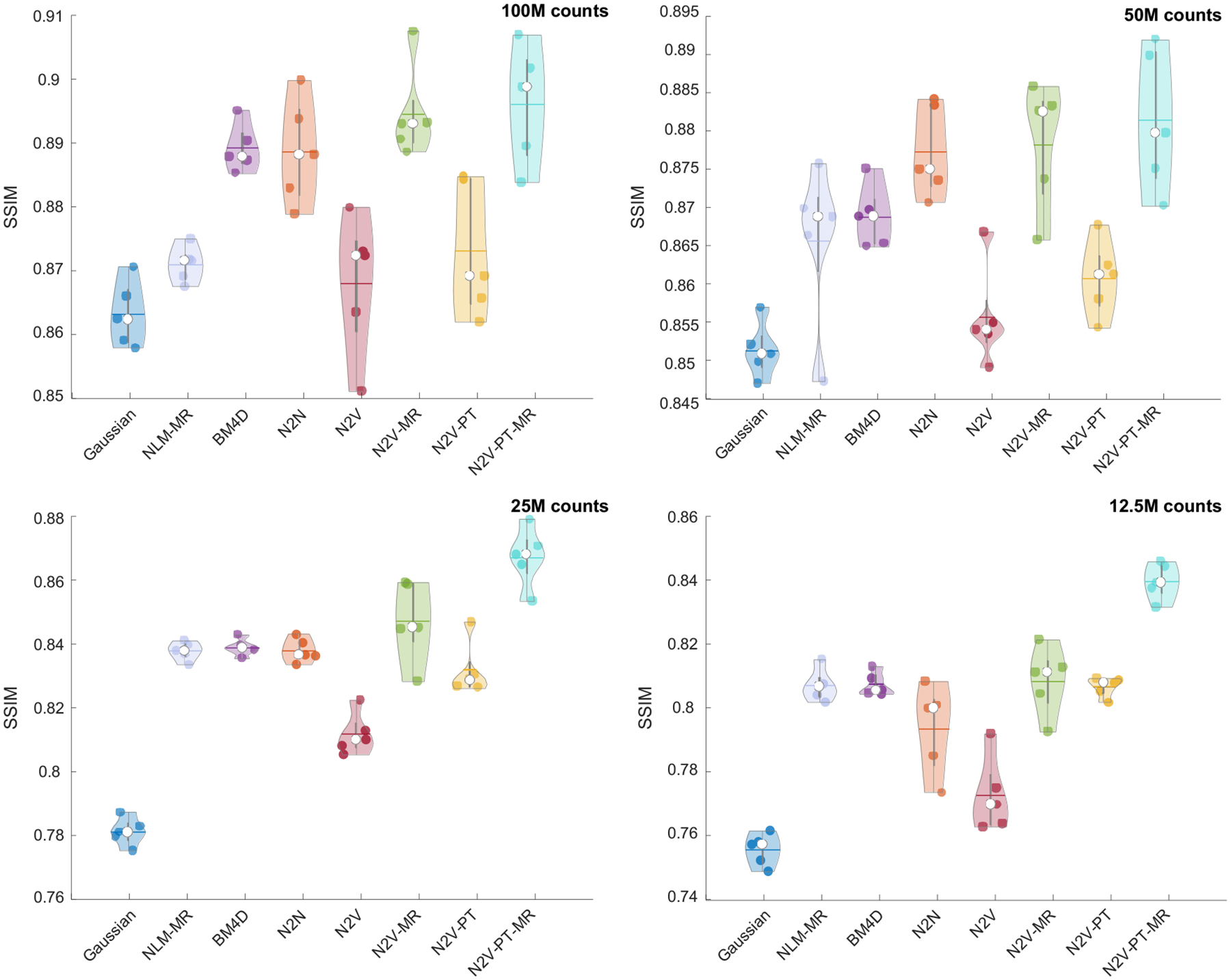
Violin plots showing the SSIM distributions for the PET images obtained using Gaussian, NLM-MR, BM4D, N2N, N2V, N2V-MR, N2V-PT, and N2V-PT-MR denoising. The results are shown for four different noise levels: 100M counts, 50M counts, 25M counts, and 12.5M counts.

Figure 5 shows sample 2D slice plots from a BrainWeb phantom belonging to the validation subset. The visualized examples have PSNR values close to the mean PSNR and correspond to the datapoints indicated as circles with a white fill in Figure 3. Transverse slices from the MR and the true (noiseless) PET are shown in the top row. The noisy and denoised images corresponding to 100M, 50M, 25M, and 12.5M simulated photon counts are displayed in the subsequent rows of the figure. Denoising results have been shown for the Gaussian, NLM-MR, BM4D, N2N, N2V, N2V-MR, N2V-PT, and N2V-PT-MR techniques. To facilitate qualitative comparison via close visual inspection of image characteristics, a part of the image (indicated by a blue box on the full-sized MR image) has been magnified and displayed in Figure 6. As expected, the Gaussian filter causes a significant amount of blurring at all noise levels. In comparison, NLM-MR leads to a sharper gray-white boundaries but shows some pixellated texture as the noise level increases. BM4D leads to low background (white matter) noise and high gray-to-white matter contrast at lower noise levels, but its performance sharply declines for high noise levels, and severe degradation of gray matter features and poor gray-to-white contrast are observed in the 12.5M counts case. N2N, which leads to consistently higher PSNR than all other methods also leads to better gray-to-white contrast than other methods for all noise levels. All N2V variants also show good gray-to-white matter contrast at all noise levels. Pretraining is particularly effective at restoring visual image quality and generates smoother and less pixellated textures in N2V-PT and N2V-PT-MR. Anatomical information (in N2V-MR and N2V-PT-MR) aids gray-white delineation and prominently reduces white matter variability. MR guidance has a noticeable impact on both high- and low-intenity regions of the image when there is no pretraining. For the pretrained cases, MR guidance has less impact on the high-intensity gray matter ROI but is instrumental at reducing the variability in the low-intensity white matter ROI. Figure 6 also shows the differences between the true and denoised PET images. From the difference images, it can be seen that N2V-MR, N2V-PT, and N2V-PT-MR lead to smaller negative differences (indicative of less underestimation of the activity) in the gray matter ROI than the N2V, NLM-MR, BM4D, and Gaussian techniques at both higher and lower noise levels.

Figure 5. Example image slices for the simulation data.

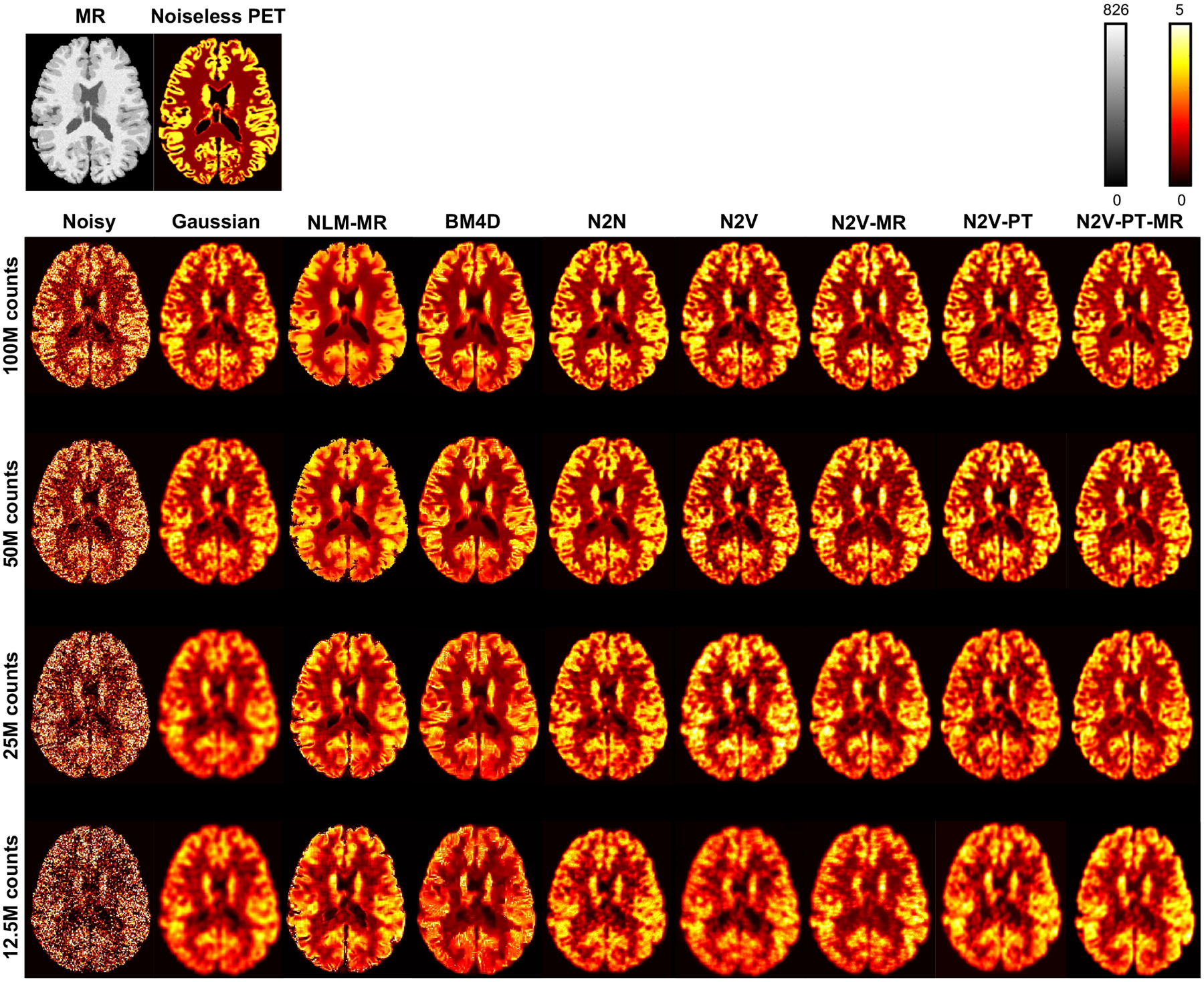
Transverse image slices from the MR and the true (noiseless) PET are shown on the top. The noisy PET images and denoised PET images based on Gaussian, NLM-MR, BM4D, N2N, N2V, N2V-MR, N2V-PT, and N2V-PT-MR are shown for four different noise levels: 100M, 50M, 25M, and 12.5M counts. The cases visualized here have PSNR values close to the mean PSNR and correspond to the datapoints indicated as circles with a white fill in Figure 3.

Figure 6. Magnified image slices and difference image slices for the simulation data.

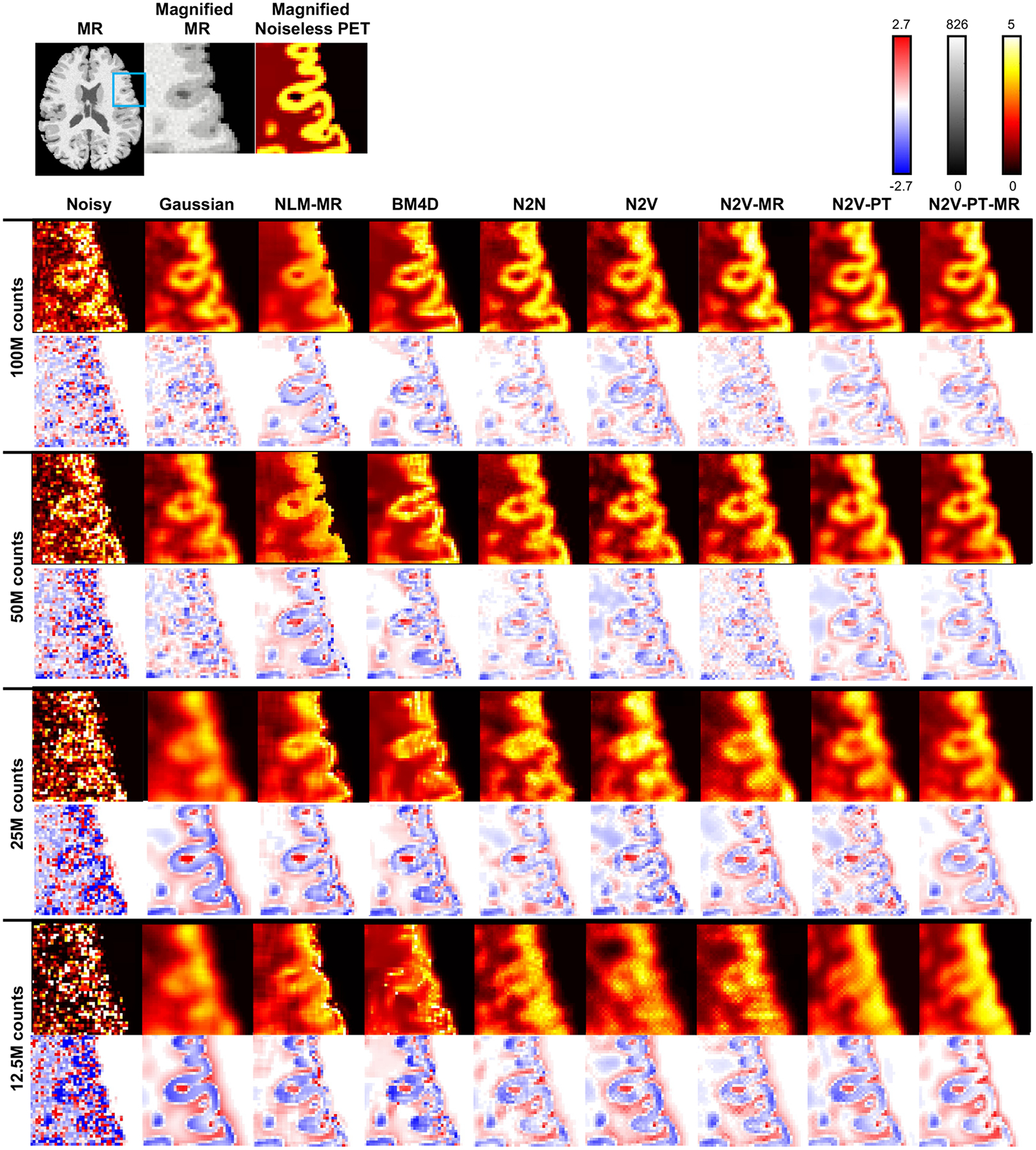
Transverse image slices from the full MR image, the magnified MR subimage, and the magnified true (noiseless) PET subimage are shown on the top row. The blue box on the full MR image indicates the region magnified for closer inspection. The noisy and denoised PET subimages are shown using a “hot” colormap for Gaussian, NLM-MR, BM4D, N2N, N2V, N2V-MR, N2V-PT, and N2V-PT-MR methods and for four different noise levels: 100M, 50M, 25M, and 12.5M counts. The corresponding difference subimages (i.e., noisy - true or denoised - true) are displayed to underneath each image slice using a red-white-blue colormap.

3.2. Clinical Results

Figure 7 shows a comparison of the PSNR obtained by applying the different denoising methods to the clinical data. For a PSNR computation, a low-noise image generated by averaging images corresponding to 6 time-frames was used as the gold-standard reference. To ensure fair comparison, we report the best value of the PSNR yielded by each method. As expected, N2N leads to the highest mean PSNR among all the methods. We should note here that the N2N result for the clinical data is based on two time-frames (the 3rd and the 4th) being used as the two noise realizations required by N2N. Among the non-deep-learning-based approaches, BM4D (32.06 dB) and NLM-MR (31.75 dB) led to higher mean PSNR than Gaussian filtering (30.68 dB). The N2V variants yielded higher PSNR than all denoising methods other than N2N. Among the N2V variants, the mean PSNR order was as follows: N2V-PT-MR (32.42 dB) > N2V-PT (32.25 dB) > N2V-MR (32.11 dB) > N2V (31.92 dB). Figure 8 shows a comparison of the SSIM obtained by applying the different denoising methods to the simulation data. N2N led to the highest SSIM overall. All N2V variants yielded higher SSIM values than the non-deep-learning-based denoisers.

Figure 7. PSNR comparison for the clinical data.

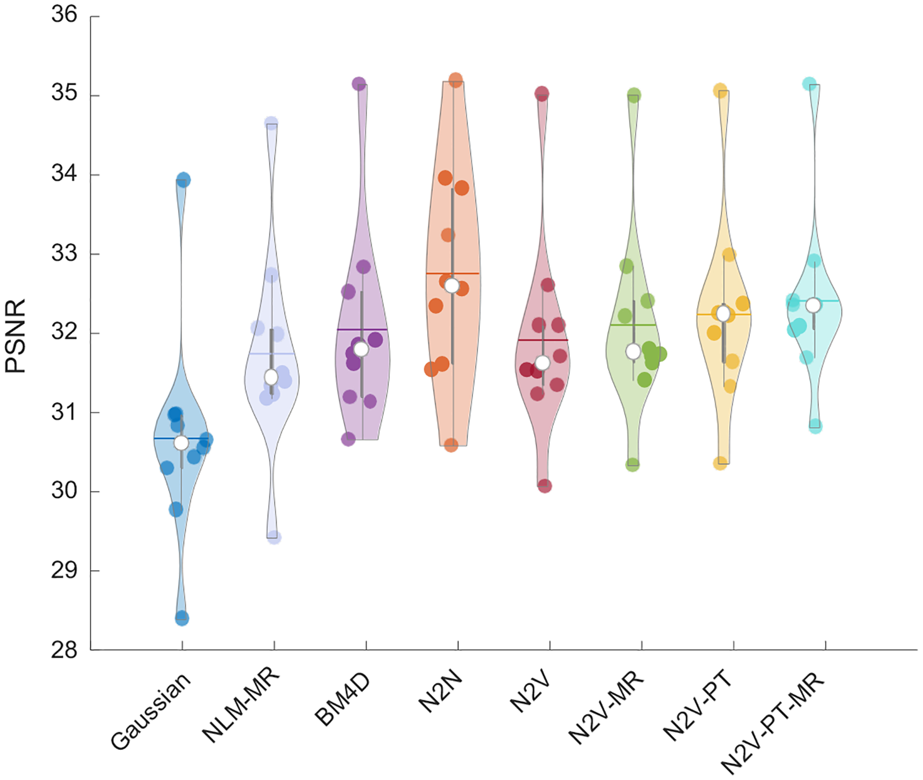
Violin plots showing the PSNR distributions for the PET images obtained using Gaussian, NLM-MR, BM4D, N2N, N2V, N2V-MR, N2V-PT, and N2V-PT-MR denoising.

Figure 8. SSIM comparison for the clinical data.

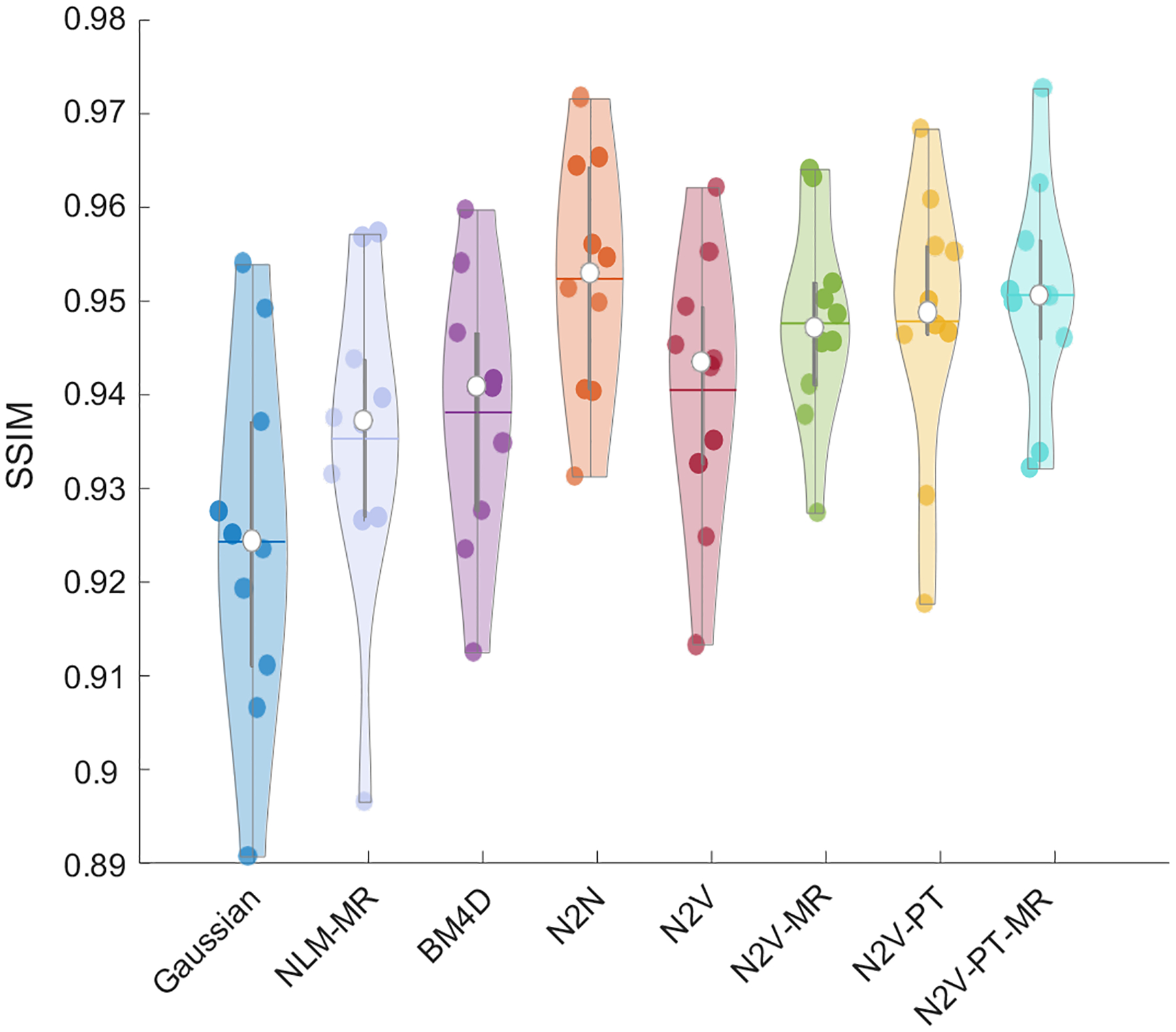
Violin plots showing the SSIM distributions for the PET images obtained using Gaussian, NLM-MR, BM4D, N2N, N2V, N2V-MR, N2V-PT, and N2V-PT-MR denoising.

Figure 9 shows sample 2D slice plots from the brain PET of a human subject from the validation subset. The visualized examples have PSNR values close to the mean PSNR and correspond to the datapoints indicated as circles with a white fill in Figure 7. Transverse slices from the MR, the noisy PET, and the low-noise PET (mean image across 6 time-frames) are shown in the top row. Denoised image slices obtained using the Gaussian, NLM-MR, BM4D, N2N, N2V, N2V-MR, N2V-PT, and N2V-PT-MR techniques are shown in the bottom row. All variants of N2V lead to low background noise in the white matter and CSF regions while largely preserving the higher intensity values of the gray matter areas. BM4D and NLM-MR seem to produce sharper features in the gray matter (purple arrows), but comparison with the low-noise image and N2N suggests that these are more likely to be noise patterns than signal patterns. To facilitate qualitative comparison via close visual inspection of image characteristics, a part of the image (indicated by a blue box on the full-sized MR image) has been magnified and displayed in Figure 10. Figure 10 also shows the differences between the low-noise and denoised PET images. While gray matter activity levels are best preserved by N2N, the pretrained N2V variants, particularly N2V-PT-MR, are also able to restore a wider high-intensity area in the gray matter (green arrows) suggestive of less underestimation.

Figure 9. Example image slices for the clinical data.

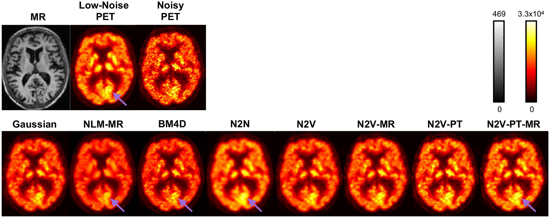
Transverse image slices from the MR, the noisy PET, and low-noise PET are shown in the top row. Transverse image slices from the denoised PET images based on the Gaussian, NLM-MR, BM4D, N2N, N2V, N2V-MR, N2V-PT, and N2V-PT-MR techniques are shown in the bottom row. The cases visualized here have PSNR values close to the mean PSNR and correspond to the datapoints indicated as circles with a white fill in Figure 7.

Figure 10. Magnified image slices and difference image slices for the clinical data.

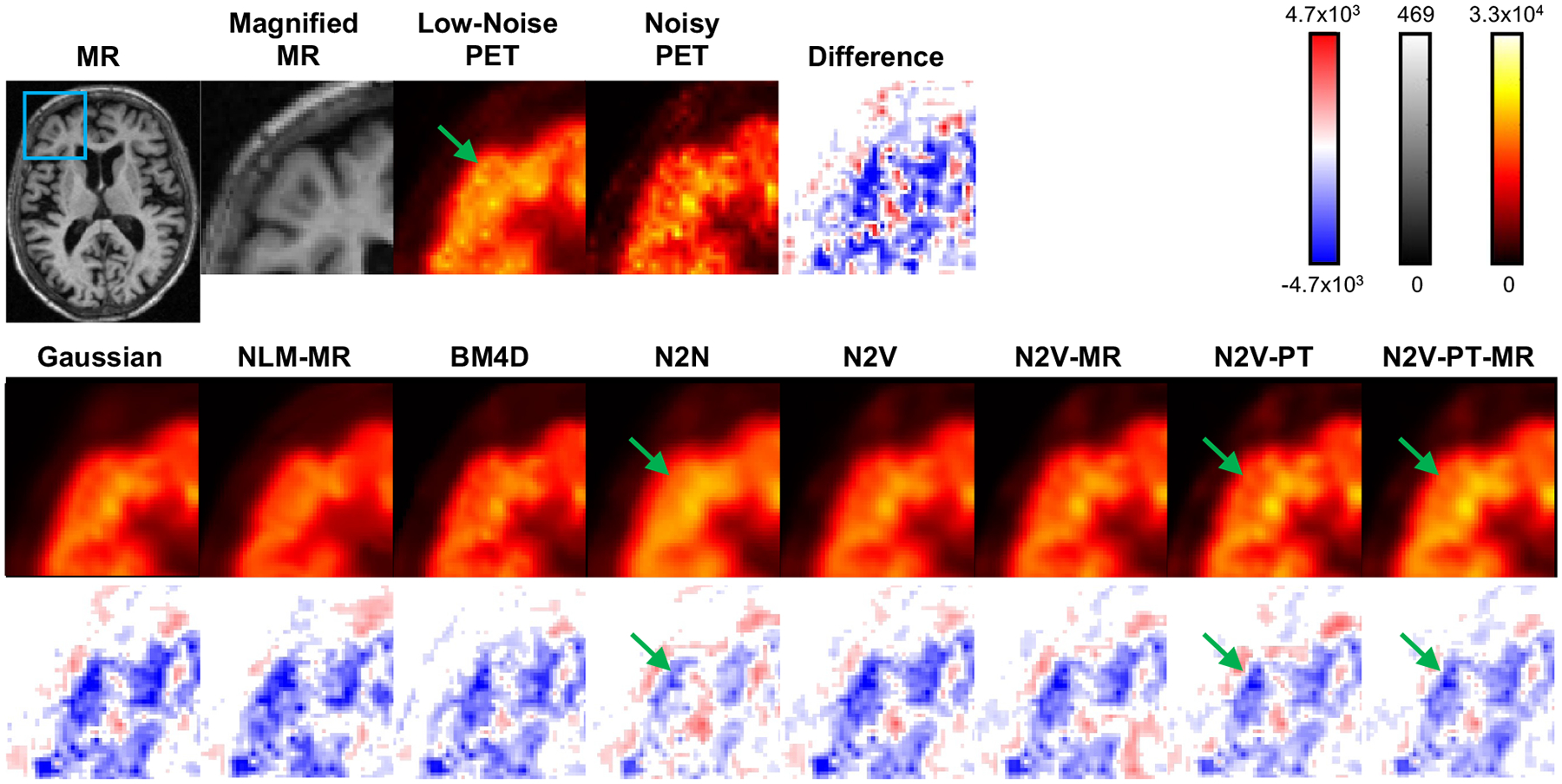
Transverse image slices from the full MR image, the magnified MR subimage, the magnified low-noise PET subimage, the magnified noisy PET subimage, and the magnified noisy PET difference subimage are shown in the top row. The blue box on the full MR image indicates the region magnified for closer inspection. Transverse image slices from the denoised PET images based on the Gaussian, NLM-MR, BM4D, N2N, N2V, N2V-MR, N2V-PT, and N2V-PT-MR techniques are shown using a “hot” colormap in the middle row. The corresponding difference subimages (i.e., denoised - true) are displayed underneath each image slice using a red-white-blue colormap.

4. Discussion

While PET has great clinical value as a molecular imaging modality, radiation dose from the radiotracer injection and extended scan times pose practical and logistical challenges for PET. Tracer dose and scan time reduction both lead to elevated noise in PET images. The high levels of noise lower the quantitative accuracy of PET. The PET image denoising problem is, therefore, one of high clinical significance. While a wide variety of neural network architectures have been developed for image denoising, the vast majority of these rely on paired low-count and high-count images for network training. Despite the high best-case accuracies of supervised methods, their clinical translational promise is diminished by the need for paired training data. In comparison, the N2V denoising technique investigated in this paper is unsupervised and, therefore, has the potential for wide adoptability.

We demonstrated here via realistic BrainWeb digital phantom simulations and ADNI brain PET data analyses that N2V denoising with pretraining and/or anatomical guidance leads to superior performance over conventional approaches like NLM-MR, BM4D, and Gaussian filtering. The margins are the highest in high-noise scenarios. While we included N2N as a reference approach, we consider it as a gold standard as it requires two noise realizations. While N2N leads to consistently higher PSNR than N2V, one should note that multiple noise realizations are not available for every clinical dataset. In comparison, unsupervised denoising methods like N2V which rely on a single noisy image have great practical utility in the clinic.

We should note here that we did not compare our method against other methods that require knowledge of ground-truth images for training (i.e., techniques that are supervised). These methods, while expected to exhibit superior performance than N2V in best-case scenarios, have practical limitations. Besides the stringent requirement of paired training data, these methods are also limited by their inability to generalize well when the training and test data have different resolution or noise characteristics. An advantage of N2V over supervised alternatives is its customizability to individual patient images since training is performed for each individual test sample. This step, however, adds some amount of computational burden, which we recognize as a limitation.

A key factor that poses a fundamental limit to the performance of an unsupervised method like N2V is its sole reliance on corrupt images for training the denoising model. When the training data is of inferior quality, it could be challenging to learn finer details of texture from the images. This challenge is offset to some extent by our pretraining strategy, which adds robustness to the approach overall. A particular vulnerability of N2V arises in some cases where a single voxel has a very different value from its neighbors. Since the blind-spot masking step assigns zero weight to the central voxel, there could be erroneous estimation of activity in such distinctive voxels. Additionally, at higher noise levels, N2V is prone to over- or underestimating activity as the model is trained without knowledge of the ground truth.

A limitation of this work is the relatively modest data size – 20 phantoms for the simulation study and 17 human subjects for the clinical study. Future investigations in much larger datasets would be needed for more thorough benchmarking of the N2V approach. In the clinical data analysis, we relied on a hybrid (simulation + clinical) dataset. Hybrid datasets consisting of both simulation and experiment data have been used for neural network training in many applications to improve model fitting in data-limited settings (Gong et al. 2019, Song et al. 2020a, Lu et al. 2021). A detailed comparison of hybrid, simulation, and clinical datasets for pretraining remains pending and will be the topic of a future investigation involving a larger dataset.

5. Conclusion

We have designed, implemented, and validated a family of denoising techniques adapted from the Noise2Void methodology, underlying which is the concept of the blind-spot network. The significance of this approach for PET image denoising lies in the fact that it is unsupervised, relies on a single noisy image, and is therefore well-suited for clinical settings. We showed that the N2V denoising performance can be improved by means of transfer learning via a pretraining step that relies only on a population of noisy images followed by fine-tuning using a single noisy image (the validation sample). We also demonstrated that the incorporation of anatomical information through an additional input channel can further improve denoising performance. This current study focused on neuroimaging datasets alone. In the future, we will extend this work to investigate the wider clinical applicability of Noise2Void. To this end, we will validate this method on a larger clinical dataset, apply it to whole-body PET data, and also apply it to data from non-FDG radiotracers.

References

- Arabi H and Zaidi H 2020. Spatially guided nonlocal mean approach for denoising of PET images Med Phys 47(4), 1656–1669. [DOI] [PubMed] [Google Scholar]
- Bergmann S, Fox K, Rand A, McElvany K, Welch M, Markham J and Sobel B 1984. Quantification of regional myocardial blood flow in vivo with Circulation 70(4), 724–733. [DOI] [PubMed] [Google Scholar]
- Boussion N, Cheze Le Rest C, Hatt M and Visvikis D 2009. Incorporation of wavelet-based denoising in iterative deconvolution for partial volume correction in whole-body PET imaging Eur J Nucl Med Mol Imaging 36(7), 1064–1075. [DOI] [PubMed] [Google Scholar]
- Buades A, Coll B and Morel JM 2005. A non-local algorithm for image denoising in ‘Computer Vision and Pattern Recognition, IEEE Computer Society Conference on’ Vol. 2 pp. 60–65. [Google Scholar]
- Chan C, Fulton R, Barnett R, Feng DD and Meikle S 2014. Postreconstruction nonlocal means filtering of whole-body PET with an anatomical prior IEEE Trans Med Imaging 33(3), 636–650. [DOI] [PubMed] [Google Scholar]
- Chan C, Zhou J, Yang L, Qi W and Asma E 2019. Noise to noise ensemble learning for PET image denoising in ‘IEEE NSS MIC’ pp. 1–3. [Google Scholar]
- Chen KT, Gong E, de Carvalho Macruz FB, Xu J, Boumis A, Khalighi M, Poston KL, Sha SJ, Greicius MD, Mormino E, Pauly JM, Srinivas S and Zaharchuk G 2020. Ultra-low-dose 18F-Florbetaben amyloid PET imaging using deep learning with multi-contrast MRI inputs Radiology 296(3), E195. [DOI] [PMC free article] [PubMed] [Google Scholar]
- Christian BT, Vandehey NT, Floberg JM and Mistretta CA 2010. Dynamic PET denoising with HYPR processing J Nucl Med 51(7), 1147–1154. [DOI] [PMC free article] [PubMed] [Google Scholar]
- Cui J, Gong K, Guo N, Wu C, Meng X, Kim K, Zheng K, Wu Z, Fu L, Xu B, Zhu Z, Tian J, Liu H and Li Q 2019. PET image denoising using unsupervised deep learning Eur J Nucl Med Mol Imaging 46(13), 2780–2789. [DOI] [PMC free article] [PubMed] [Google Scholar]
- da Costa-Luis CO and Reader AJ 2021. Micro-networks for robust MR-guided low count PET imaging IEEE Trans Radiat Plasma Med Sci 5(2), 202–212. [DOI] [PMC free article] [PubMed] [Google Scholar]
- Dabov K, Foi A, Katkovnik V and Egiazarian K 2007. Image denoising by sparse 3-D transform-domain collaborative filtering IEEE Trans Image Process 16(8), 2080–2095. [DOI] [PubMed] [Google Scholar]
- Delbeke D et al. 1999. Oncological applications of FDG PET imaging: brain tumors, colorectal cancer lymphoma and melanoma J Nucl Med 40, 591–603. [PubMed] [Google Scholar]
- Dutta J, Ahn S and Li Q 2013. Quantitative statistical methods for image quality assessment Theranostics 3(10), 741–756. [DOI] [PMC free article] [PubMed] [Google Scholar]
- Dutta J, Leahy RM and Li Q 2013. Non-local means denoising of dynamic PET images PLoS ONE 8(12), e81390. [DOI] [PMC free article] [PubMed] [Google Scholar]
- El Fakhri G, Sitek A, Guérin B, Kijewski M, Di Carli M and Moore S 2005. Quantitative dynamic cardiac 82Rb PET using generalized factor and compartment analyses J Nucl Med 46(8), 1264–1271. [PubMed] [Google Scholar]
- Farde L, Eriksson L, Blomquist G and Halldin C 1989. Kinetic analysis of central [11C] raclopride binding to D2-dopamine receptors studied by PET – A comparison to the equilibrium analysis J Cereb Blood Flow Metab 9(5), 696–708. [DOI] [PubMed] [Google Scholar]
- Farwell MD, Pryma DA and Mankoff DA 2014. PET/CT imaging in cancer: current applications and future directions Cancer 120(22), 3433–3445. [DOI] [PubMed] [Google Scholar]
- Gong K, Guan J, Liu C and Qi J 2019. PET image denoising using a deep neural network through fine tuning IEEE Trans Radiat Plasma Med Sci 3(2), 153–161. [DOI] [PMC free article] [PubMed] [Google Scholar]
- He K, Sun J and Tang X 2013. Guided image filtering IEEE Trans Pattern Anal Mach Intell 35(6), 1397–1409. [DOI] [PubMed] [Google Scholar]
- Hofheinz F, Langner J, Beuthien-Baumann B, Oehme L, Steinbach J, Kotzerke J and van den Hoff J 2011. Suitability of bilateral filtering for edge-preserving noise reduction in PET EJNMMI Res 1(1), 23. [DOI] [PMC free article] [PubMed] [Google Scholar]
- Krull A, Buchholz T and Jug F 2019. Noise2Void – Learning denoising from single noisy images in ‘IEEE/CVF CVPR’ pp. 2124–2132. [Google Scholar]
- Le Pogam A, Hanzouli H, Hatt M, Cheze Le Rest C and Visvikis D 2013. Denoising of PET images by combining wavelets and curvelets for improved preservation of resolution and quantitation Med Image Anal 17(8), 877–891. [DOI] [PubMed] [Google Scholar]
- Lehtinen J, Munkberg J, Hasselgren J, Laine S, Karras T, Aittala M and Aila T 2018. Noise2Noise: Learning image restoration without clean data in ‘ICML’ Vol. 80 pp. 2965–2974. [Google Scholar]
- Lin JW, Laine AF and Bergmann SR 2001. Improving PET-based physiological quantification through methods of wavelet denoising IEEE Trans Biomed Eng 48(2), 202–212. [DOI] [PubMed] [Google Scholar]
- Liu CC and Qi J 2019. Higher SNR PET image prediction using a deep learning model and MRI image Phys Med Biol 64(11), 115004. [DOI] [PMC free article] [PubMed] [Google Scholar]
- Lu T, Chen T, Gao F, Sun B, Ntziachristos V and Li J 2021. LV-GAN: A deep learning approach for limited-view optoacoustic imaging based on hybrid datasets J Biophotonics 14(2), e202000325. [DOI] [PubMed] [Google Scholar]
- Ote K, Hashimoto F, Kakimoto A, Isobe T, Inubushi T, Ota R, Tokui A, Saito A, Moriya T, Omura T, Yoshikawa E, Teramoto A and Ouchi Y 2020. Kinetics-induced block matching and 5-D transform domain filtering for dynamic PET image denoising IEEE Trans Radiat Plasma Med Sci 4(6), 720–728. [Google Scholar]
- Ronneberger O, Fischer P and Brox T 2015. U-Net: Convolutional networks for biomedical image segmentation arXiv preprint arXiv:1505.04597 [Google Scholar]
- Salmon E, Bernard Ir C and Hustinx R 2015. Pitfalls and limitations of PET/CT in brain imaging Semin Nucl Med 45(6), 541–551. [DOI] [PubMed] [Google Scholar]
- Schaefferkoetter J, Yan J, Ortega C, Sertic A, Lechtman E, Eshet Y, Metser U and Veit-Haibach P 2020. Convolutional neural networks for improving image quality with noisy PET data EJNMMI Res 10(1), 105. [DOI] [PMC free article] [PubMed] [Google Scholar]
- Song TA, Chowdhury SR, Yang F and Dutta J 2020a. PET image super-resolution using generative adversarial networks Neural Netw 125, 83–91. [DOI] [PMC free article] [PubMed] [Google Scholar]
- Song TA, Chowdhury SR, Yang F and Dutta J 2020b. Super-resolution PET imaging using convolutional neural networks IEEE Trans Comput Imaging 6, 518–528. [DOI] [PMC free article] [PubMed] [Google Scholar]
- Tauber C, Stute S, Chau M, Spiteri P, Chalon S, Guilloteau D and Buvat I 2011. Spatio-temporal di usion of dynamic PET images Phys Med Biol 56(20), 6583–6596. [DOI] [PubMed] [Google Scholar]
- Wang Y, Yu B, Wang L, Zu C, Lalush DS, Lin W, Wu X, Zhou J, Shen D and Zhou L 2018. 3D conditional generative adversarial networks for high-quality PET image estimation at low dose Neuroimage 174, 550–562. [DOI] [PMC free article] [PubMed] [Google Scholar]
- Wang Z, Bovik AC, Sheikh HR and Simoncelli EP 2004. Image quality assessment: from error visibility to structural similarity IEEE Trans. Image Process 13(4), 600–612. [DOI] [PubMed] [Google Scholar]
- Xu J, Gong E, Pauly J and Zaharchuk G 2017. 200× Low-dose PET reconstruction using deep learning arXiv preprint arXiv:1712.04119 [Google Scholar]
- Yan J, Lim JC and Townsend DW 2015. MRI-guided brain PET image filtering and partial volume correction Phys Med Biol 60(3), 961–976. [DOI] [PubMed] [Google Scholar]
- Yie SY, Kang SK, Hwang D and Lee JS 2020. Self-supervised PET denoising Nucl Med Mol Imaging 54(6), 299–304. [DOI] [PMC free article] [PubMed] [Google Scholar]
- Zhou L, Schaefferkoetter JD, Tham IWK, Huang G and Yan J 2020. Supervised learning with CycleGAN for low-dose FDG PET image denoising Med Image Anal 65, 101770. [DOI] [PubMed] [Google Scholar]