Improved Performance of a Multipinhole SPECT for DAT Imaging by Increasing Number of Pinholes at the Expense of Increased Multiplexing

Abstract

SPECT imaging of dopamine transporters (DAT) in the brain is a widely utilized study to improve the diagnosis of Parkinsonian syndromes, where conventional (parallel-hole and fan-beam) collimators on dual-head scanners are commonly employed. We have designed a multi-pinhole (MPH) collimator to improve the performance of DAT imaging. The MPH collimator focuses on the striatum and hence offers a better trade-off for sensitivity and spatial resolution than the conventional collimators within this clinically most relevant region for DAT imaging. Our original MPH design consisted of 9 pinholes with a background-to-striatal (Bkg/Str) projection multiplexing of 1% only. In this simulation study, we investigated whether further improvements in the performance of MPH imaging could be obtained by increasing the number of pinholes, hence by enhancing the sensitivity and sampling, despite the ambiguity in reconstructing images due to increased multiplexing. We performed analytic simulations of the MPH configurations with 9, 13, and 16 pinholes (aperture diameters: 4–6mm) using a digital phantom modeling DAT imaging. Our quantitative analyses indicated that using 13 (Bkg/Str: 12%) and 16 (Bkg/Str: 22%) pinholes provided better performance than the original 9-pinhole configuration for the acquisition with 2 or 4 angular views, but a similar performance with 8 and 16 views.

I. Introduction

Dopamine transporter (DAT) I-123-ioflupane single photon emission tomography (SPECT) is a widely utilized study to improve the diagnostic accuracy of Parkinsonian syndromes, which can be clinically challenging to separate from other neurologic disorders given the overlap of signs and symptoms [1]. Additionally, clinical trials have increasingly utilized DAT-SPECT for monitoring progression of Parkinson disease [2]. The target region for DAT imaging is the striatum, a small structure in the central part of the brain, composed of putamen and caudate nuclei. DAT imaging is typically performed using general-purpose dual-head SPECT cameras with low-energy high-resolution (LEHR) parallel-hole (or fanbeam, if available) collimators, as recommended by the European Association of Nuclear Medicine, EANM [3, 4] and the Society of Nuclear Medicine and Molecular Imaging, SNMMI [5] guidelines. However, spatial resolution and sensitivity offered by these collimators are not optimal for DAT imaging as large portion of the detector area remains unused because of the smaller size of the brain compared to the detectors. This low sensitivity results in unnecessarily long scan durations lasting typically between 30–45 minutes. Hence, both EANM and SNMMI guidelines also recommend dedicated systems for I-123 DAT imaging, if available.

A number of dedicated brain SPECT designs, employing mainly cone-beam or pinhole collimators and various detector sizes and shapes, have been developed to improve the sensitivity and spatial-resolution tradeoff for better imaging performance in the brain [6–13]. Computer-based simulations [14–16] and real acquisitions [17–19] of some of these dedicated systems have shown superior performance for DAT imaging over the usage of the conventional (i.e., parallel-hole and fanbeam) collimators on general-purpose scanners.

With similar motivations, we have proposed a multi-pinhole (MPH) collimator specifically designed to improve the performance of DAT imaging by replacing the conventional collimators on a dual-head SPECT system. Unlike many other dedicated brain systems, our MPH covers a smaller field-of-view (FOV) including the striatum rather than the entire brain to further improve the trade-off between sensitivity and spatial resolution within this region. In a previous study, we have shown that 9- and 16-pinhole MPH collimators with 5 mm diameter apertures provide about 3 and 5 times higher striatal counts, respectively compared to a parallel-hole LEHR collimator [20]. Our original MPH collimator with 9 pinholes was designed to have a minimal background-to-striatal projection overlap (Bkg/Str multiplexing of 1%) [21, 22], as in many other MPH collimator designs to avoid artifacts in reconstructions from the ambiguity created by the multiplexed data. However, numerous publications have indicated that artifact-free reconstructions from multiplexed data are achievable depending on the system and imaging task, especially if non-multiplexed data are available and/or sampling is sufficient, as summarized in a review paper by Van Audenhaege et al (and the references in) [23] and in [14]. If the non-multiplexed data are not available, the effects of multiplexing can be reduced by using a de-multiplexing approach, as described in [24], which incorporates an additional iterative procedure in the reconstruction. Another approach for handling multiplexing proposed the usage of a dedicated MPH system made by stacking silicon (Si) and germanium (Ge) detectors, where “little multiplexed Si projections” help reducing the artifacts from the “highly multiplexed Ge projections” [25].

Motivated by these findings, we investigated whether we could obtain further improvements in the performance of our original MPH collimator design by increasing the number of pinholes, hence enhancing sensitivity and sampling (angular and axial), at the expense of increased multiplexing. For this purpose, we performed a series of analytic simulations of DAT imaging using MPH configurations with 9, 13, and 16 pinholes for aperture diameters of 4, 5, and 6 mm.

II. Methods

A. DAT Phantom

We used the XCAT digital phantom [26] to model the distributions of the I-123-ioflupane in the brain for DAT imaging with striatum:background activity concentration ratios of 8:1 and 4:1, which are among the typical ratios seen in the clinic [27], covering normal and decreased striatum uptake due to the disease and/or aging [28].

We generated non-uniform random backgrounds [29] in the brain to approximately model the variation in uptake [30] by applying a 3D Gaussian filter (σ = 2 mm) after adding white Gaussian noise (signal-to-noise ratio = 1) to the uniform background for all the distributions investigated herein, as shown in Fig. 1. This resulted in about ±10% variation in the background, and about ±1.25% and ±2.5% variations in the striatum for a contrast ratio (CR) of 8 and 4, respectively, as the striatum was added over the non-uniform background.

Fig. 1.

Steps for generating the non-uniform background in the DAT activity phantom. The activity in the striatum was then added over this phantom.

B. Simulations of the MPH Collimators

We performed analytic simulations of the MPH configurations with 9, 13, and 16 knife-edge pinholes all focusing on the center of the FOV (CFOV), referred to as 9MPH, 13MPH and 16MPH, respectively, for the aperture diameters of 4, 5, and 6 mm. These MPH configurations and aperture sizes were narrowed down from our previous studies covering a larger number of combinations [31, 32]. Herein, the plane at which all the pinhole centers are located is defined as the aperture plane, which is parallel to the detector plane. The aperture plane-to-detector and the axis-of-rotation (AOR)-aperture plane distances were 17.25 and 14 cm, respectively, providing an image magnification of ~1.23 for all the pinholes at the CFOV, which is located over the AOR.

The planar spatial resolutions listed in Table I were measured from the projections of a point source at the CFOV and averaged over all the pinholes in the horizontal and vertical directions. The sensitivities calculated using the geometric sensitivity equation described in [33] at the CFOV are also listed in this table. Herein, the geometric sensitivity of the 9MPH with 4 mm diameter circular knife-edge apertures was 0.034%. The geometric sensitivity of the previously studied 9MPH with the same pinhole positions and orientations, but with 2.2 mm knife-edge square-apertures was 0.013% [22].

Table I.

Multiplexing, sensitivity, and planar resolution

Collimators	9MPH			13MPH			16MPH
Bkg/Str %		0.7			12			22
Bkg/Bkg %		11			27			35
Pinhole ∅	4mm	5mm	6mm	4mm	5mm	6mm	4mm	5mm	6mm
Relative Sensitivity	1	1.5	2.2	1.4	2.2	3.2	1.6	2.6	3.6
Geometric Sensitivity%	0.034	0.053	0.076	0.048	0.075	0.108	0.054	0.084	0.122
*Res (mm)	7.4	8.8	10.8	7.2	9.0	10.3	7.1	8.9	10.3
Total Counts	1.6M	2.5M	3.6M	2.3M	3.5M	5.1M	2.6M	4.1M	5.8M

^*Planar resolutions at the center of the FOV averaged over all the pinhole projections in horizontal and vertical directions.

We set the acceptance angles of all the MPH configurations such that we can maintain the coverage of the FOV for the 9MPH (diameter: ~12 cm and height:~8 cm). The pinhole acceptance angles for the 9MPH ranged from 38° to 43° (bottom row of pinholes: 43°- 48°- 43°, middle row: 38°- 40°- 38°, and top row: 40°- 40°- 40°). The 13MPH had the same acceptance angles for the similarly positioned nine pinholes. The acceptance angles for the extra four pinholes in the 13MPH and for all the 16MPH pinholes were set to 40°.

To assess the importance of the number of angular views in the reconstructed image quality, we simulated projection datasets over different number of angular views (n) of 2, 4, 8, and 16, providing a total of 9 × n, 13 × n, and 16 × n unique views for 9MPH, 13MPH, and 16MPH, respectively. Fig. 2 shows these MPH configurations and their corresponding noise-free projections of the DAT phantom obtained from a 16-view acquisition and summed over all the views. As illustrated, the cameras were simulated as stationary in 90° mode for the 2-view acquisition, while the rest of the acquisitions were obtained in 180° mode with equally separated angular views over 360°.

Fig. 2.

MPH configurations and their noise-free projections for the DAT tracer distribution for CR=8. The projections shown here are summed over 360° using the 16-view acquisition mode as illustrated (right) along with the other modes. The stationary 2-view acquisition was in 90° mode while the rest of the acquisitions were in 180° mode.

C. Multiplexing Calculations

We designed all three MPH collimator configurations to have no striatal-to-striatal (Str/Str) multiplexing to avoid an ambiguity in the images for the main region of interest (ROI) in DAT imaging. Then based on separate projections of the background (non-striatal) and striatal components (caudate, putamen, and substantia nigra) of the DAT phantom source distribution, we determined the regions with background-to-background (Bkg/Bkg) and background-to-striatal (Bkg/Str) multiplexing using binary masks. The Bkg/Bkg and Bkg/Str multiplexing percentages over all projection angles were calculated as following:

$$\text{Multiplexing}\%\text{=100}\times \frac{{\sum }_{\text{proj }}\text{num}.\text{of pixels in multiplexed regions}}{{\sum }_{\text{proj }}\text{num}.\text{of pixels of non-zero regions}}$$ (1)

Note, the small amount of additional Bkg/Bkg multiplexing occurring among a set of three neighboring pinholes (i.e., 3-way intersections in Fig. 2) for the 13MPH and 16MPH configurations was not taken into account in the multiplexing calculations.

Table I summarizes the multiplexing percentages obtained from the 16-view projections of the DAT phantom using (1). Note, the multiplexing measurements were nearly independent of the pinhole diameters, hence we presented the values based on the 5 mm pinholes only.

D. Count Levels, Projections, and Reconstructions

We set the total acquired counts of the 9MPH with 4 mm diameter apertures to be 1.6 million, slightly higher than the minimum counts recommended by the SNMMI guidelines [5], which corresponds to 30–45 minutes of scan time for a typical injection of 185 MBq activity with the conventional SPECT acquisitions. The count levels of the other cases were determined based on the relative sensitivities obtained from the DAT phantom projections for equal acquisition time and the same activity distribution. The relative sensitivities and the total acquired counts are listed in Table I. Based on the geometric sensitivity of the 9MPH-4mm system relative to that of a parallel-hole LEHR collimator on a dual-head SPECT system with an 8 mm resolution at the CFOV [34, 35]. we estimate that the count levels listed in this table could be obtained at half of the imaging time of that system. Note, the dead time between the different acquisition angles needed for the detector head rotation was not simulated in this study, which would result in slightly increased total scan durations as the number of rotation steps increases.

For the simulations and reconstructions, we used an in-house GPU-accelerated analytic simulation and iterative reconstruction software for MPH systems that shared the same forward projector using multi-ray tracing for the emission and single-ray tracing for the attenuation modeling/correction [36]. The software modeled the MPH collimator geometry, object attenuation (scatter in object and system was not modeled), effective aperture diameters for resolution and sensitivity [37, 38], and the detector intrinsic resolution of 3 mm. The same physical and geometrical properties were modeled in forward and back-projectors. Therefore, the same effects and properties modeled in the simulation were corrected for in the reconstruction, including attenuation modeling and its correction using XCAT-based attenuation map. Poisson noise was applied to the noise-free projections to obtain five noise realizations for each case studied, which were then reconstructed using a maximum-likelihood expectation-maximization (MLEM) algorithm for 100 iterations [39].

The phantom matrix was 240×240×240 with a voxel size of (1 mm)³. The projection matrix was 200×270 with a pixel size of (2 mm)² corresponding to the axial and lateral detector dimensions of 400 and 540 mm, respectively. The reconstruction matrix was 120×120×120, with a voxel size of (2 mm)³. The reconstructed images were post-smoothed by a 3D Gaussian filter with standard deviation ranging from 0.5 mm to 2 mm with increments of 0.5 mm.

E. Error Quantification within the FOV

As a metric of image reconstruction fidelity, we used the normalized root-mean-square error (NRMSE) of the reconstruction values within a spherical volume of 8 cm diameter centered at the CFOV, which included the entire striatum. This region is smaller than the cylindrical FOV to avoid potential boundary effects. NRMSE was calculated as

$$\text{NRMSE}=\sqrt{\frac{{\sum }_{\text{i}}{\left(\text{Ref}\left(\text{i}\right)-\text{Recon}(\text{i})\right)}^2}{{\sum }_{\text{i}}{\left(\text{Ref}\left(\text{i}\right)\right)}^2}}$$ (2)

where, Ref(i) and Recon(i) are the ground truth (reference) and reconstructed image values, respectively, at the voxel index i. Note, the reference phantom matrix was down-sampled to the matrix size of the reconstruction. We reported the average of the NRMSE values over 5 noise realizations.

F. Bias and Variance Measurements

We calculated bias as a measure of accuracy and coefficient of variation (CV) as a measure of deviation from the mean value. We expressed bias as,

$$\text{Bias}(\%)=100\times \frac{\text{abs}\left({\text{Str}}_{\text{ref}}-{\text{Str}}_{\text{meas}}\right)}{{\text{Str}}_{\text{ref}}}$$ (3)

where mean reference (Str_ref) and mean striatum measurement (Str_meas) were obtained over the entire striatum using its known template from the reference phantom. CV% = 100 × σ/μ was calculated within an elliptical background region, where σ and μ are standard deviation and mean, respectively. We reported the average of these values over 5 noise realizations.

G. Quantifications using clinical metrics

The usage of semi-quantitative methods in DAT imaging forms an important part of the clinical evaluation. For this purpose, we calculated striatal-binding ratio (SBR), a measure of striatal specific binding relative to the non-specific binding, which is a clinically relevant quantitative task [40]. SBR is calculated as (Str – Occ) / Occ, where Str and Occ are the mean activity concentrations in the striatum and occipital regions measured from the reconstructed slices, respectively. We combined the normalized errors in the striatum and background measurements (NSB_err) in a single equation based on the square differences of the reference and measured values in the respective regions:

$${\text{NSB}}_{\text{err}}=\sqrt{\frac{{\left({\text{Str}}_{\text{meas}}-{\text{Str}}_{\text{ref}}\right)}^2}{{\text{Str}}_{\text{ref}}{}^2}+\frac{{\left({\text{Bkg}}_{\text{meas}}-{\text{Bkg}}_{\text{ref}}\right)}^2}{{\text{Bkg}}_{\text{ref}}{}^2}}$$ (4)

Here, the mean reconstructed (Str_meas) and reference (Str_ref) values were obtained over the central three slices in the striatum, where at each slice the ROI was set to be slightly smaller than the striatum to reduce the impact of the partial volume effect (PVE) [41]. We determined the ROI by applying a 3-pixel image erosion operation to the striatum template at the corresponding slices. Note, with this choice Str_ref value, obtained from down-sampled phantom, was nearly equal to the true striatum value (Str_true). For the mean background measurement (Bkg_meas) and reference (Bkg_ref), we used an elliptical ROI within the FOV close to the the occipital region, as our MPH system covers a limited FOV.

In addition to the SBR, we obtained caudate-to-putamen ratios (CP), as another semi-quantitative parameter [42]. Similar to (4), the combined error (NCP_err) in caudate (Cau) and putamen (Put) was obtained as below:

$${\text{NCP}}_{\text{err}}=\sqrt{\frac{{\left({\text{Cau}}_{\text{meas}}-{\text{Cau}}_{\text{ref}}\right)}^2+{\left({\text{Put}}_{\text{meas}}-{\text{Put}}_{\text{ref}}\right)}^2}{{\left({\text{Str}}_{\text{ref}}\right)}^2}}$$ (5)

A 2-pixel image erosion operation was applied to these regions. Our analyses are based on the average of the NSB_err and NCP_err over 5 noise realizations.

III. Results

Fig. 3 shows the Bkg/Bkg and Bkg/Str binary masks for a sample projection view. The corresponding multiplexing percentages obtained from (1) are displayed on each projection image (also listed in Table I).

Fig. 3.

Binary Bkg/Bkg and Bkg/Str masks for a sample projection view with the multiplexing percentages displayed.

As determined from 16-view acquisitions, σ =1 mm for the 3D-Gaussian postfiltering resulted in the lowest NRMSE values for all aperture sizes and MPH configurations, which were up to ~3% lower than the case of no filtering. Therefore, all the reconstructions and analyses herein are based on this selection.

Fig. 4 shows the NRMSE plots calculated within the 8 cm diameter spherical region over 100 iterations for the 2-view and 16-view acquisitions and for the CR=8 and 4. As the number of angular views increased from 2 to 16, the minimum NRMSE over iterations decreased because of the improved angular sampling. In general, NRMSE values were lower for the cases with higher sensitivity. For example, 16MPH with 5 mm and 6 mm diameter apertures had the lowest NRMSEs. For the 2-view, 16MPH with 6 mm apertures had the lowest NRMSEs.

Fig. 4.

Mean NRMSE plots over 5 noise realizations calculated within the 8 cm diameter spherical region at the CFOV for the 2-view and 16-view acquisitions and for the CR=8 and 4. The insert shows the outline of the spherical ROI (colored region inside the solid line circle) and the imaging FOV (white dashed circle) overlaid on the DAT phantom summed over axial slices.

Fig. 5 shows the scatter plots of Bias% and CV% over 100 iterations for the CR=8 and 4. In general, 16-view mode provided lower bias and variation in uptake. For most cases, MPH16 with 5 and 6mm apertures provided better trade-off between the bias and variance.

Fig. 5.

The scatter plots of the bias% versus coefficient of variation (CV%) calculated within the entire striatum and background regions, respectively, for the 2-view and 16-view acquisitions and for the CR=8 and 4. The insert shows the ROI (colored) for the calculations and the imaging FOV (white dashed circle) overlaid on the phantom image summed over axial slices.

Fig. 6 shows the NSB_err defined in (4) for the CR=8 and 4. The insert in the figure shows the ROIs for the striatum and background regions over summed images of the phantom. Three central slices were selected for both regions located at different slice depths. In general, the 16-view acquisition mode provided lower NSB_err, where 9MPH with smaller apertures were favored. For the 2-view mode, 16MPH performed better. The scatter plots in Fig. 7 show the mean values measured in the striatum and the background regions for the CR=8 and 4. The yellow circles indicate the true values for both regions (e.g., for CR=8, mean(Str)=8 and mean(Bkg)=l). The reference values used in (4) were slightly lower than these true values as the down-sampling from the true phantom reduced the pixel values around the boundary of the striatum. The estimation of the absolute values for both contrast ratios were dramatically improved with the 16 angular views, where the 9MPH with 4 mm and 5 mm apertures provided the best combined values for the striatum and background ROIs.

Fig. 6.

NSB_err calculated within the three central slices of the striatum and background regions for the 2-view and 16-view acquisitions and for the CR=8 and 4. The insert shows the ROIs (colored) for the calculations and the imaging FOV (white dashed circle) overlaid on the phantom image summed over axial slices.

Fig. 7.

The scatter plots for the mean(Str) versus mean(Bkg) over 100 iterations calculated within the three central slices of the striatum and background regions for CR=8 and 4. The yellow circles indicate the true values for both regions. The insert shows the ROIs (colored) for the calculations and the imaging FOV (white dashed circle) overlaid on the phantom image summed over axial slices.

Fig. 8 shows a subset of the axial reconstructed slices from 4-view and 16-view acquisitions for a sample noise realization at the center of the striatum and at the iteration corresponding to the lowest NSB_err for CR=8 and 4. Each image is linearly scaled between zero to its own peak. Visually, the images were of similar quality except for the more obvious differences between the 2-view and 16-view acquisition modes, which were more apparent for the CR=4. The SBR values labeled under each slice confirm these differences quantitatively. For the CR=8 (SBR_true = 7), SBR ranged from 3.5–5.2 and 7.3–8.1 for the 2-view and 16-view acquisitions, respectively. For the CR=4 (SBR_true = 3), the corresponding ranges were 1.2–1.8 and 2.8–3.1. Hence, the variation in quantitative SBR performance among the different collimators were more meaningful for the 2-view compared to the 16-view. The line profiles through the striatum are also shown for the lowest NSB_err within a set of 9 images, where the image quality and quantification obtained with 16 views was better than that of 2 views. Also, 9MPH had the lowest NSB_err for the 4 (CR=8) and 5 mm (CR=4) apertures.

Fig. 8.

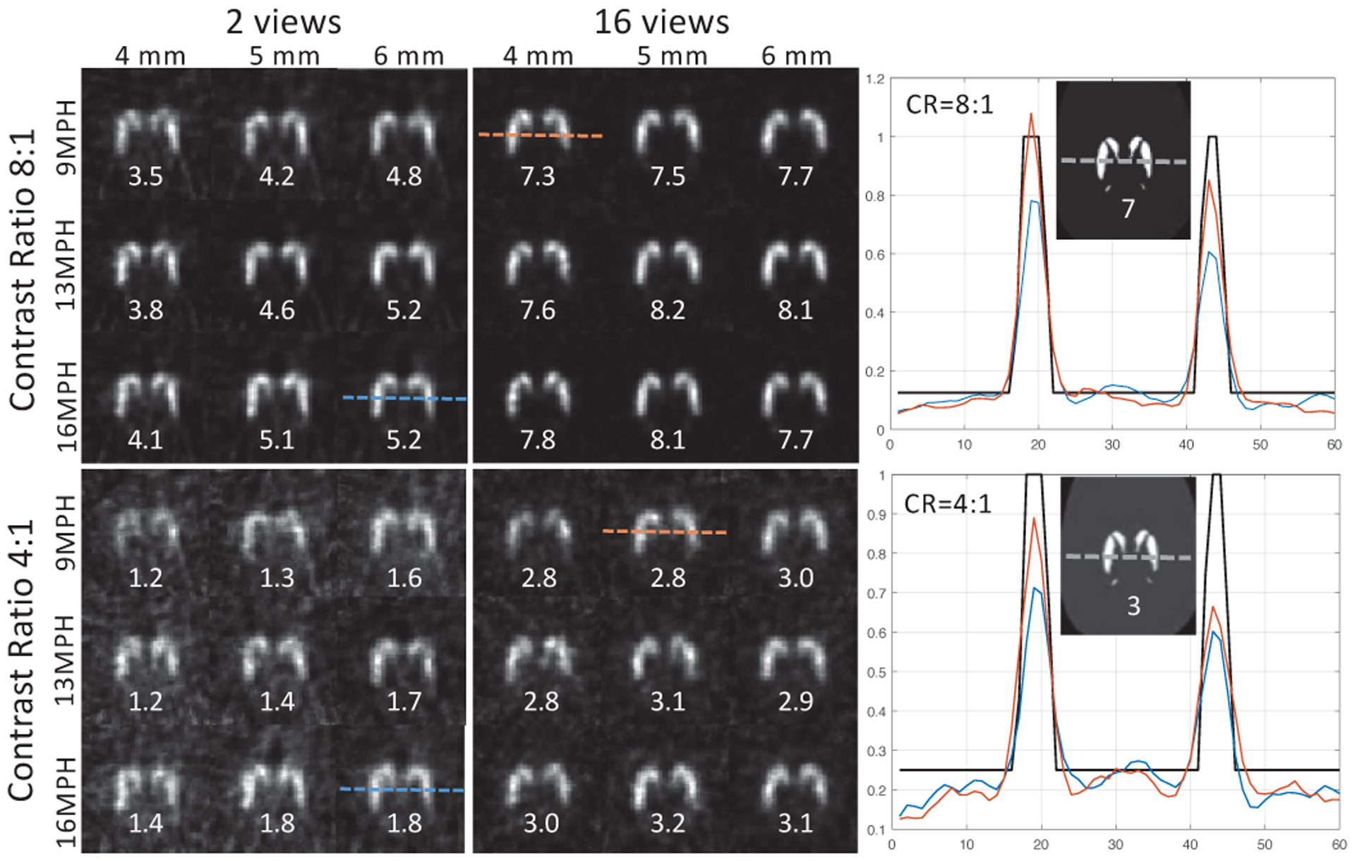
Axial reconstructed slices for a sample noise realization through the center of the striatum at the iteration corresponding to the lowest NSB_err. Each image is linearly scaled between zero to its own peak value. The measured (SBR_meas) and reference (SBR_ref) values are labeled under the corresponding images. Note, the lowest NSB_err does not necessarily provide SBR_meas closest to the SBR_ref. Line profiles through the striatum are shown with the lowest NSB_err within each set of 9 images.

IV. Discussion

We presented an analytical simulation study of various MPH configurations with different aperture sizes and under different imaging conditions as detailed in the previous sections. Determining an optimized collimator design with a specific aperture size is challenging because of the confounding factors such as source distribution, ROI, pinhole positions and orientations in the aperture plate, angular and axial sampling, truncation, multiplexing, spatial resolution, and system sensitivity. Nevertheless, this study aims to provide guidance for determining the MPH collimator parameters.

Fig. 9 presents a summary of the results based on the lowest errors obtained for NRMSE, NSB, and NCP quantitative metrics considered in this study. Note, this figure also includes the lowest errors for the 4-view and 8-view acquisition modes, which were not included in the previous figures.

Fig. 9.

Summary plots showing the lowest NRMSE within the FOV (a), lowest NSB_err within the striatum and background (b), and lowest NCP_err within the striatum (c), for CR=8 (indicated with circled markers) and CR=4 (no circle). The inserts in each subfigure shows the calculations performed in the corresponding ROIs (colored) and the imaging FOV (white dashed circle) overlaid on the phantom image summed over axial slices.

Overall, the error values for all the metrics reported herein decreased as the number of angular views increased from 2 to 16, as can be expected because of the improved angular sampling. However, because of the small ROIs and the availability of many projection views (angular views × number of pinholes), 8-view mode appears to perform generally similar to 16-view acquisition mode. Also, the range of errors for the lower number of angular views (e.g., 2-view) were more spread and hence were more meaningful compared to the larger number of angular views.

We presented NRMSE plots within the FOV (Fig. 4) to evaluate the fidelity of the reconstructed images with the ground truth. Fig. 9(a) shows the lowest NRMSEs from these plots, where 13MPH and 16MPH collimators with 5 mm and 6 mm diameter apertures performed slightly better for all the acquisition modes. This suggests that the gain in sensitivity obtained with the usage of larger size and more pinholes overcomes the impact of multiplexing and poor spatial resolution within the FOV. In addition to the gain in sensitivity, more pinholes also offer improved sampling.

The NRMSE combines bias and variance into a single metric. Therefore, to study their individual contributions to the overall error, we calculated the bias and variance separately and presented their scatter plots in Fig. 5. A small portion of this bias is related to the slight non-uniformity in the striatum as explained in Methods (up to ±2.5%). However, the main reason for the elevated errors was due to the PVE as the spatial resolution provided by the apertures were not sufficient to resolve the thin portions of the striatum. Nevertheless, for the semi-quantitative metrics this effect can be partially mitigated by using the counts in a smaller volume of the striatum avoiding the boundaries and thin portions, as shown herein with the SBR and CP calculations. Note, we applied different levels of erosion to SBR (3-pixel) and CP (2-pixel) to maintain a similar magnitude of error, as CP with 3-pixel erosion was providing about 10-fold less errors resulting in insignificant differences in error levels among different cases of MPH.

While the visual image quality was better for the CR=8, NRMSE and CV% values were lower for CR=4. The reason for this is the smaller difference between the signal and background for the case of CR=4. As the difference decreases, the image approaches to uniformity. For example, as an extreme case, NRMSE and CV% would reach to the lowest values in the absence of a signal (i.e., CR=1). Hence, NRMSE and CV% values from these two different contrast ratios should be regarded separately.

In addition to the metrics presented above, we obtained SBR calculations as a clinically relevant metric. SBR, however, is a semi-quantitative metric (a measure of uptake ratio) and thus it does not necessarily indicate the quantitative accuracy of the striatum and background regions. For example, the true SBR value could be obtained even from very poor-quality reconstructed images with inaccurate quantifications at the early iterations. Therefore, for a more meaningful performance evaluation, we presented the mean(Str) and mean(Bkg) values used in the SBR calculation (Fig. 7) and combined their corresponding errors into a single error value as NSB_err (Fig. 6). We then presented the reconstructed images obtained at iterations with the lowest NSB_err, which resulted in relatively accurate SBR values (Fig. 8).

Fig. 9(b) shows the lowest NSB_err values obtained from the data presented in Fig. 6. For the 2-view and 4-view acquisition modes, 16MPH with 5 mm and 6 mm apertures performed the best in accurate estimation of SBR for both contrast ratios. For the 16-view acquisition, however, 9MPH with 4 mm and 5 mm apertures appeared to perform better than most other cases although the error levels and their differences were very low. Also, interestingly the error level recorded in 8-view was similar and, in some cases, smaller than the NSB_err recorded with the 16-view. This indicates that when the angular sampling is sufficient, the count density (counts/view), hence the quality (less noisy) of each projection, may become more relevant than additional views.

For the SBR calculation, the background measurement is commonly obtained from the occipital cortex as the dopamine receptors are negligible in this region compared to the striatum [43]. In this study, because of the limited FOV offered by our MPH design, we obtained the background measurements from a region close to the occipital cortex, which was within the FOV and hence closer to the striatum. Note, in our original combined system design (i.e., combined usage of an MPH and a conventional collimator in a dual-head acquisition protocol), the main role of the conventional collimator was to provide a reliable quantification from the occipital region. However, if an alternative region such as mentioned here and/or a region posterior to the striatum produces similar background measurements, an MPH-only system similar to other dual-head [14] or triple-head [44] MPH systems could be considered over our original combined design. With such an approach a stationary imaging of the striatum appears possible (axial slices with 2 views in Fig. 8), but likely with reduced fidelity (plots in Fig. 4) and quantitative accuracy (plots in Fig. 6–8).

Another potential concern for the small FOV is the effect of truncated emission data in making accurate quantitative measurements due to the interior reconstruction problem. That is, values in a reconstruction within a fully sampled convex interior region are accurately reconstructed only to an additive constant, unless there is a small sub-region within the interior region whose values are exactly known and constrained to match during reconstruction. Thus, our accuracy in this work is limited to an unknown, possibly small additive constant [45], as observed in this study (Fig. 7).

The areas containing cerebrospinal fluid such as cerebral ventricles are known to have no tracer uptake [46], hence their reconstructed values would be expected to be close to zero. However, we determined that the ventricles within the FOV were on average 30% of the background and 7.5% of the striatum true values for the 16MPH collimator with 5mm apertures using 16 angular views. We then obtained projections and reconstructions of the same phantom using another MPH collimator design with 7 pinholes whose apertures we selected to result in the same spatial resolution, and which fully sample the entire brain [47] avoiding the interior problem. In this case the reconstructed values in the ventricles were 22% of the background and 5.5% of the striatum true values. Hence, the differences in these percentages for the two reconstructions were 8% and 2% for the background and striatum, which can be attributed to the interior problem assuming the same level of bias from PVE for both MPH systems. We therefore conclude that, for the structures of interest in DAT striatal imaging, the effect of the interior problem on our quantitative results is small compared to the bias introduced by the PVE. We also assume that our attenuation map is obtained from a CT, for example on a SPECT/CT system, and is not truncated. Thus, we avoid the case where both emission data and attenuation map are truncated.

An alternative to the SBR is the usage of the CP [48, 49], which does not require background measurements. This may be a reasonable approach considering the progression of Parkinson’s Disease typically starts in the posterior part of one of the putamen [50] and thus the diagnosis mainly depends on the putamen/caudate ratios in the right and left striatum [51]. Hence, as another clinically relevant metric, we obtained CP values (not shown) and their errors (only the lowest errors are shown in Fig 9). Fig. 9(c) shows the lowest NCP_err. For the 16-view acquisition, the 16MPH with 4 mm and 5 mm apertures appear to perform slightly better than the 9MPH or 13MPH for this metric due to more counts with more pinholes.

The results in this study are supporting the usage of additional pinholes with larger diameters for the acquisition modes with the fewer number of angles. All the quantitative metrics we investigated herein indicates that 13MPH and 16MPH with 5 mm and 6 mm aperture diameters are performing consistently better than all the other cases for the 2-view and 4-view acquisition modes. Also, in more cases 16MPH with 6 mm provided slightly lower errors. While with the current setup the error levels are higher for these two acquisition modes, more specific collimator designs and/or camera angles could reduce these errors. Also, 2-view stationary imaging have many advantages: enhanced resolution and sensitivity in striatum region as the aperture planes could potentially get closer to the patient head in stationary mode; increased patient safety and comfort; dynamic imaging although in a small FOV; potentially less patient motion; easier motion tracking and correction; and no imaging dead time between different acquisition angles, which may become more relevant for shorter total acquisition times with the MPH collimator approach. 4-view acquisition shares these advantages to some extent as it requires just a single rotation step.

Based on the quantitative metrics studied herein, additional pinholes do not necessarily improve the imaging performance for the 8-view and 16-view acquisition modes. The sampling advantage of the additional pinholes is apparent when there are only few angular views. For example, for the 2-view mode, while 9MPH has only 18 total views, 16MPH provides 32 total views, greatly improving the sampling needs. As the number of angular views increases, however, the need for sampling decreases, hence the importance of the additional pinholes. When larger number of angular views are available, the advantage of additional pinholes essentially reduces to higher sensitivity, which appears to barely balance the impact of multiplexing, as can be seen from very small differences in error levels presented among different cases. Nevertheless, for both 13MPH and 16MPH configurations, a further improvement could be obtained by the implementation of a de-multiplexing algorithm to reduce the artifacts originating from multiplexing [24], or usage of temporal shuttering of apertures to provide usage of a portion of the imaging time with multiplexing free imaging [16, 52].

While our original MPH collimator was designed to work in combination with a conventional collimator, in this work we focused on improving the performance of the MPH component only, which is expected to translate in the performance of the overall combined system. With a combined system, multiplexing may be better handled because of the complete dataset available from the conventional collimator, as reported for example in [53], and the avoidance of the interior reconstruction problem [45].

V. Conclusion

We determined through a series of analytic simulations that additional pinholes (going from 9 to 13 and 16 pinholes) can further improve the DAT imaging performance of our two-headed MPH-SPECT system for the 2-view stationary and 4-view (solely 1 rotation) acquisition modes. Thus, with a limited number of angular views, the increase in sampling and sensitivity with additional pinholes improved imaging performance despite the larger amount of multiplexing in the projections. Overall, 16MPH with 6 mm provided the lowest errors for the 2-view and 4-view acquisitions. Altering the pinhole positions slightly and adjusting camera views to improve the angular and axial sampling, can be also considered, which is especially important when limited number of projection views are used.

Overall the 16-view acquisition mode (with the 8-view nearly the same) provided the best performance by our metrics with only small differences among the MPHs with different number of pinholes. This indicates that with sufficient number of angular views, the benefit offered by the additional pinholes were limited, likely due to the increased multiplexing. While for the 8-view and 16-view modes we observed no considerable performance improvement with the additional pinholes, de-multiplexing algorithms and/or usage of combined multiplexed and non-multiplexed data in reconstruction, may result in quantitative improvements.

References

- [1].Ogawa T et al. , “Role of Neuroimaging on Differentiation of Parkinson’s Disease and Its Related Diseases,” Yonago Acta Med, vol. 61, no. 3, pp. 145–155, September 2018. [DOI] [PMC free article] [PubMed] [Google Scholar]
- [2].Scherfler C et al. , “Role of DAT-SPECT in the diagnostic work up of parkinsonism,” Mov Disord, vol. 22, no. 9, pp. 1229–38, July 15 2007. [DOI] [PubMed] [Google Scholar]
- [3].Darcourt J et al. , “EANM procedure guidelines for brain neurotransmission SPECT using (123)I-labelled dopamine transporter ligands, version 2,” Eur J Nucl Med Mol Imaging, vol. 37, no. 2, pp. 443–50, February 2010. [DOI] [PubMed] [Google Scholar]
- [4].Morbelli S et al. , “EANM practice guideline/SNMMI procedure standard for dopaminergic imaging in Parkinsonian syndromes 1.0,” Eur J Nucl Med Mol Imaging, vol. 47, no. 8, pp. 1885–1912, July 2020. [DOI] [PMC free article] [PubMed] [Google Scholar]
- [5].Djang DS et al. , “SNM practice guideline for dopamine transporter imaging with 123I-ioflupane SPECT 1.0,” J Nucl Med, vol. 53, no. 1, pp. 154–63, January 2012. [DOI] [PubMed] [Google Scholar]
- [6].Johnston BA, Nicol A, Bolster A, and Wright J, “Development and validation of a full model of a four-headed neuroimaging single-photon emission computed tomography scanner,” Nucl Med Commun, vol. 40, no. 1, pp. 14–21, January 2019. [DOI] [PMC free article] [PubMed] [Google Scholar]
- [7].Sensakovic WF, Hough MC, and Kimbley EA, “ACR testing of a dedicated head SPECT unit,” J Appl Clin Med Phys, vol. 15, no. 4, p. 4632, July 8 2014. [DOI] [PMC free article] [PubMed] [Google Scholar]
- [8].Park M et al. , “Introduction of a novel ultrahigh sensitivity collimator for brain SPECT imaging.,” Med Phys, vol. 43, no. 8, p. 4734, 2016. [DOI] [PMC free article] [PubMed] [Google Scholar]
- [9].Zito F, Savi A, and Fazio F, “CERASPECT: a brain-dedicated SPECT system. Performance evaluation and comparison with the rotating gamma camera,” Phys Med Biol, vol. 38, pp. 1433–1442, 1993. [Google Scholar]
- [10].Beekman FJ et al. , “G -SPECT-I: a full ring high sensitivity and ultrafast clinical molecular imaging system with < 3mm resolution,” presented at the EANM, 2015. [Google Scholar]
- [11].El Fakhri G, Ouyang J, Zimmerman RE, Fischman AJ, and Kijewski MF, “Performance of a novel collimator for high-sensitivity brain SPECT,” Med Phys, vol. 33, no. 1, pp. 209–15, January 2006. [DOI] [PubMed] [Google Scholar]
- [12].Mahmood ST, Erlandsson K, Cullum I, and Hutton BF, “Design of a novel slit-slat collimator system for SPECT imaging of the human brain,” Phys Med Biol, vol. 54, no. 11, pp. 3433–49, June 7 2009. [DOI] [PubMed] [Google Scholar]
- [13].Zeraatkar N et al. , “Preliminary Investigation of Axial and Angular Sampling in Multi-Pinhole AdaptiSPECT-C with XCAT Phantoms,” IEEE NSS/MIC, 2017. [Google Scholar]
- [14].Chen L, Tsui BMW, and Mok GSP, “Design and evaluation of two multi-pinhole collimators for brain SPECT,”Ann Nucl Med, vol. 31, no. 8, pp. 636–648, October 2017. [DOI] [PubMed] [Google Scholar]
- [15].Chen Y, Vastenhouw B, Wu C, Goorden MC, and Beekman FJ, “Optimized image acquisition for dopamine transporter imaging with ultra-high resolution clinical pinhole SPECT,” Phys Med Biol, vol. 63, no. 22, p. 225002, November 7 2018. [DOI] [PubMed] [Google Scholar]
- [16].Zeraatkar N et al. , “Investigation of Axial and Angular Sampling in Multi-Detector Pinhole-SPECT Brain Imaging,” IEEE Trans Med Imaging, vol. PP, August 7 2020. [DOI] [PMC free article] [PubMed] [Google Scholar]
- [17].Tecklenburg K et al. , “Performance evaluation of a novel multi-pinhole collimator for dopamine transporter SPECT,” Phys Med Biol, May 5 2020. [DOI] [PubMed] [Google Scholar]
- [18].Park MA et al. , “Introduction of a novel ultrahigh sensitivity collimator for brain SPECT imaging,” Med Phys, vol. 43, no. 8, p. 4734, August 2016. [DOI] [PMC free article] [PubMed] [Google Scholar]
- [19].Lee TC, Ellin JR, Huang Q, Shrestha U, Gullberg GT, and Seo Y, “Multipinhole collimator with 20 apertures for a brain SPECT application,” Med Phys, vol. 41, no. 11, p. 112501,November 2014. [DOI] [PMC free article] [PubMed] [Google Scholar]
- [20].Konik A et al. , “Primary, scatter, and penetration characterizations of parallel-hole and pinhole collimators for I-123 SPECT,” Phys Med Biol, vol. 64, no. 24, p. 245001, December 13 2019. [DOI] [PMC free article] [PubMed] [Google Scholar]
- [21].King MA, Mukherjee JM, Konik A, Zubal IG, Dey J, and Licho R, “Design of a Multi-Pinhole Collimator for I-123 DaTscan Imaging on Dual-Headed SPECT Systems in Combination with a Fan-Beam Collimator,” IEEE Trans Nucl Sci, vol. 63, no. 1, pp. 90–97, February 2016. [DOI] [PMC free article] [PubMed] [Google Scholar]
- [22].Könik A et al. , “Simulations of a Multi-Pinhole SPECT Collimator for Clinical Dopamine Transporter (DAT) Imaging,” IEEE Trans Rad Plasma Med Sci, 2018. [DOI] [PMC free article] [PubMed] [Google Scholar]
- [23].Van Audenhaege K, Van Holen R, Vandenberghe S, Vanhove C, Metzler SD, and Moore SC, “Review of SPECT collimator selection, optimization, and fabrication for clinical and preclinical imaging,” Med Phys, vol. 42, no. 8, pp. 4796–813, August 2015. [DOI] [PMC free article] [PubMed] [Google Scholar]
- [24].Moore SC, Cervo M, Metzler SD, Udias JM, and Herraiz J. n. L., “An Iterative Method for Eliminating Artifacts from Multiplexed Data in Pinhole SPECT,” in Fully Three-Dimensional Image Reconstruction in Radiology and Nuclear Medicine, 2015, [Google Scholar]
- [25].Johnson LC, Shokouhi S, and Peterson TE, “Reducing multiplexing artifacts in multi-pinhole SPECT with a stacked silicon-germanium system: a simulation study,” IEEE Trans Med Imaging, vol. 33, no. 12, pp. 2342–51, December 2014. [DOI] [PMC free article] [PubMed] [Google Scholar]
- [26].Segars WP, Sturgeon G, Mendonca S, Grimes J, and Tsui BM, “4D XCAT phantom for multimodality imaging research,” (in eng), Med Phys, vol. 37, no. 9, pp. 4902–15, September 2010. [DOI] [PMC free article] [PubMed] [Google Scholar]
- [27].Dickson JC et al. , “The impact of reconstruction method on the quantification of DaTSCAN images,” Eur J Nucl Med Mol Imaging, vol. 37, no. 1, pp. 23–35, January 2010. [DOI] [PubMed] [Google Scholar]
- [28].Nicastro N, Garibotto V, Poncet A, Badoud S, and Burkhard PR, “Establishing On-Site Reference Values for (123)I-FP-CIT SPECT (DaTSCAN(R)) Using a Cohort of Individuals with Non-Degenerative Conditions,” Mol Imaging Biol, vol. 18, no. 2, pp. 302–12, April 2016. [DOI] [PubMed] [Google Scholar]
- [29].Konik A, Kupinski M, Pretorius PH, King MA, and Barrett HH, “Comparison of the scanning linear estimator (SLE) and ROI methods for quantitative SPECT imaging,” Phys Med Biol, vol. 60, no. 16, pp. 6479–94, August 21 2015. [DOI] [PMC free article] [PubMed] [Google Scholar]
- [30].G. G and R. A, “What Can SPECT Learn from Autoradiography?,” in Proc. IEEE NSS/MIC, 1994, vol. 4, pp. 1715–1719. [Google Scholar]
- [31].Könik A et al. , “Preliminary Investigation of Multiplexed Pinholes with Circular Apertures and Elliptical Ports for I-123 DAT Imaging,” in IEEE NSS/MIC, 2017. [Google Scholar]
- [32].Könik A, Mukherjee JM, Banerjee S, Beenhouwer JD, Zubal GI, and King MA, “Optimization of Pinhole Aperture Size of a Combined MPH/FanBeam SPECT System for I-123 DAT Imaging,” in NSS/MIC, 2016. [Google Scholar]
- [33].Mallard JR and Myers MJ, “The performance of a gamma camera for the visualization of radioactive isotope in vivo,” Phys Med Biol, vol. 8, pp. 165–82, June 1963. [DOI] [PubMed] [Google Scholar]
- [34].Nillius P and Danielsson M, “Theoretical bounds and system design for multipinhole SPECT,” IEEE Trans Med lmaging, vol. 29, no. 7, pp. 1390–400, July 2010. [DOI] [PubMed] [Google Scholar]
- [35].Goorden MC, Rentmeester MC, and Beekman FJ, “Theoretical analysis of full-ring multi-pinhole brain SPECT,” Phys Med Biol, vol. 54, no. 21, pp. 6593–610, November 7 2009. [DOI] [PubMed] [Google Scholar]
- [36].Zeraatkar N, Auer B, Kalluri K, Furenlid LR, Kuo PH, and King MA, “ GPU-accelerated generic analytic simulation and image reconstruction platform for multi-pinhole SPECT systems,” Fully Three-Dimensional Image Reconstruction in Radiology and Nuclear Medicine (SPIE), 2019. [Google Scholar]
- [37].Accorsi R and Metzler SD, “Analytic determination of the resolution-equivalent effective diameter of a pinhole collimator,” IEEE Trans Med Imaging, vol. 23, no. 6, pp. 750–63, June 2004. [DOI] [PubMed] [Google Scholar]
- [38].Accorsi R and Metzler SD, “Resolution-effective diameters for asymmetric-knife-edge pinhole collimators,” IEEE Trans Med Imaging, vol. 24, no. 12, pp. 1637–46, December 2005. [DOI] [PubMed] [Google Scholar]
- [39].Shepp LA and Vardi Y, “Maximum likelihood reconstruction for emission tomography,” IEEE Trans Med Imaging, vol. 1, no. 2, pp. 113–22, 1982. [DOI] [PubMed] [Google Scholar]
- [40].Kuo PH et al. , “Receiver-operating-characteristic analysis of an automated program for analyzing striatal uptake of 123I-ioflupane SPECT images: calibration using visual reads,” J Nucl Med Technol, vol. 41, no. 1, pp. 26–31, March 2013. [DOI] [PubMed] [Google Scholar]
- [41].Kessler RM, Ellis JR Jr., and Eden M, “Analysis of emission tomographic scan data: limitations imposed by resolution and background,” J Comput Assist Tomogr, vol. 8, no. 3, pp. 514–22, June 1984. [DOI] [PubMed] [Google Scholar]
- [42].Matesan M et al. , “I-123 DaTscan SPECT Brain Imaging in Parkinsonian Syndromes: Utility of the Putamen-to-Caudate Ratio,” J Neuroimaging, vol. 28, no. 6, pp. 629–634, November 2018. [DOI] [PubMed] [Google Scholar]
- [43].Lamelle M et al. , “SPECT imaging of striatal dopamine release after amphetamine challenge,” J Nucl Med, vol. 36, no. 7, pp. 1182–90, July 1995. [PubMed] [Google Scholar]
- [44].Ogawa K and Ichimura Y, “Simulation study on a stationary data acquisition SPECT system with multi-pinhole collimators attached to a triple-head gamma camera system,” Ann Nucl Med, vol. 28, no. 8, pp. 716–24, October 2014. [DOI] [PubMed] [Google Scholar]
- [45].Zeng GL and Gullberg GT, “Exact iterative reconstruction for the interior problem,” Phys Med Biol, vol. 54, no. 19, pp. 5805–14, October 7 2009. [DOI] [PMC free article] [PubMed] [Google Scholar]
- [46].Catafau AM, “Brain SPECT in clinical practice. Part I: perfusion,” J Nucl Med, vol. 42, no. 2, pp. 259–71, February 2001. [PubMed] [Google Scholar]
- [47].Konik A et al. , “Design of a dual-head multi-pinhole collimator for brain SPECT with improved axial sampling,” in J Nucl Med, 2018, vol. 59, [Google Scholar]
- [48].Shin HY, Kang SY, Yang JH, Kim HS, Lee MS, and Sohn YH, “Use of the Putamen/Caudate Volume Ratio for Early Differentiation between Parkinsonian Variant of Multiple System Atrophy and Parkinson Disease,” Journal οf clinical neurology, vol. 3, no. 2, pp. 79–81, June 2007. [DOI] [PMC free article] [PubMed] [Google Scholar]
- [49].Soderlund TA et al. , “Value of semiquantitative analysis for clinical reporting of 123I-2-beta-carbomethoxy-3beta-(4-iodophenyl)-N-(3-fluoropropyl)nortropane SPECT studies,” J Nucl Med, vol. 54, no. 5, pp. 714–22, May 2013. [DOI] [PubMed] [Google Scholar]
- [50].Kuo PH, Eshghi N, Tinaz S, Blumenfeld H, Louis ED, and Zubal G, “Optimization of Parameters for Quantitative Analysis of (123)I-Ioflupane SPECT Images for Monitoring Progression of Parkinson Disease,” J Nucl Med Technol, vol. 47, no. 1, pp. 70–74, March 2019. [DOI] [PubMed] [Google Scholar]
- [51].Brooks DJ, “Imaging approaches to Parkinson disease,” J Nucl Med, vol. 51, no. 4, pp. 596–609, April 2010. [DOI] [PubMed] [Google Scholar]
- [52].Van Audenhaege K, Vandenberghe S, Deprez K, Vandeghinste B, and Van Holen R, “Design and simulation of a full-ring multi-lofthole collimator for brain SPECT,” Phys Med Biol, vol. 58, no. 18, pp. 6317–36, September 21 2013. [DOI] [PubMed] [Google Scholar]
- [53].Vunckx K, Suetens P, and Nuyts J, “Effect of overlapping projections on reconstruction image quality in multipinhole SPECT,” IEEE Trans Med Imaging, vol. 27, no. 7, pp. 972–83, 2008. [DOI] [PubMed] [Google Scholar]