Methods for the segmentation and classification of breast ultrasound images: a review

Abstract

Purpose

Breast ultrasound (BUS) is one of the imaging modalities for the diagnosis and treatment of breast cancer. However, the segmentation and classification of BUS images is a challenging task. In recent years, several methods for segmenting and classifying BUS images have been studied. These methods use BUS datasets for evaluation. In addition, semantic segmentation algorithms have gained prominence for segmenting medical images.

Methods

In this paper, we examined different methods for segmenting and classifying BUS images. Popular datasets used to evaluate BUS images and semantic segmentation algorithms were examined. Several segmentation and classification papers were selected for analysis and review. Both conventional and semantic methods for BUS segmentation were reviewed.

Results

Commonly used methods for BUS segmentation were depicted in a graphical representation, while other conventional methods for segmentation were equally elucidated.

Conclusions

We presented a review of the segmentation and classification methods for tumours detected in BUS images. This review paper selected old and recent studies on segmenting and classifying tumours in BUS images.

Introduction

Ultrasound (US) uses sound waves to produce images of internal structures of the body. Analysts use image processing techniques (such as segmentation, enhancement, and classification) to detect affected areas in ultrasound images. Segmentation algorithms divide images into segments and extract a region of interest (ROI). Recently, image segmentation algorithms are on the increase owing to the advancements in information technology. References [1–4] opined that recent image segmentation techniques involve the use of advanced mathematical methods. The use of advanced computer algorithms to segment medical images automatically generates the ROI [5].

Breast ultrasound (BUS) is one of the cheapest imaging modalities in clinical medicine. Primarily, it aims to diagnose breast lumps or other abnormalities during physical examination. In addition, BUS is safe and does not produce radiation, and it is used as a supplement to mammograms to improve the rate of cancer detection and to reduce false-negative occurrences [6–8]. Clinical abnormalities detected by BUS could be malignant or benign, such as fibroadenomas and cysts (see details in [9–13]). Interestingly, breast-cancer-related diseases are tumour problems; the old cells do not die when the new cells are created. Electromagnetic interference to the body might be a breast-cancer-causing agent (carcinogens). The electromagnetic waves in mobile phones, telecommunication masts, and other electromagnetic components could be carcinogens. Furthermore, breast-cancer-related problems have made the world a darker place. Individuals living with breast cancer are in pain or face an early death. The use of alcohol and cigarettes contributes to cancer. Genetics and family-related problems can also contribute to cancer. Luckily, several techniques and medical procedures have been developed to address breast-cancer-related problems. In the light of the aforementioned challenges, it is imperative to understand the techniques of breast cancer diagnosis. Hence, this paper examines various techniques and methods for diagnosing breast cancer.

This paper is organised as follows. The section “Literature review” provides a background to the fundamental principles of BUS segmentation and classification. The section “BUS datasets” discusses BUS datasets, and the section “Analyses” describes the analyses. Finally, we conclude the paper in the section “Conclusions and future directions”.

Literature review

Manual segmentation is the gold standard; however, it is time-consuming and laborious [14–16]. To overcome these limitations, several automatic segmentation methods have been proposed [17]. In this paper, BUS segmentation approaches are divided into four categories: (1) graph-based methods, (2) other methods, (3) traditional methods, and (4) semantic segmentation methods. The first three categories comprise popular approaches, while the last category contains new methods that are increasingly used. A block diagram depicting the different approaches for BUS segmentation is shown in Fig. 1.

Fig. 1.

BUS segmentation approaches

In addition, several methods exist for classifying BUS images. Interestingly, most of these classifiers are closely related to segmentation methods, which are intermittently used as a classifier. Some classifiers use domain expert algorithms to recognise classes. Others use statistical similarity algorithms to group clusters (see Fig. 2; Table 1).

Fig. 2.

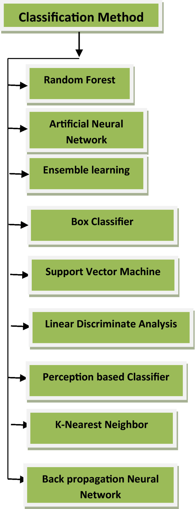
BUS classification methods

Table 1.

Acronym and meaning

Acronym	Meaning
SPC	Specificity
TPF	True-positive fraction
JS	Jaccard similarity
ASM	Area similarity measure
BF1	Boundary F1 scores
SR	Similarity ratio
TPVF	True-positive volume fraction
TP	True positive
APR	Area precision rate
ACC	Accuracy
DSC	DICE similarity coefficient
SEN	Sensitivity

Approaches for the segmentation of BUS images

Traditional methods

First, we review various thresholding algorithms. In Reference [18], the authors proposed a two-stage thresholding fuzzy entropy algorithm. The first stage involved the selection of a cancer region based on the level-set algorithm [19], and the second stage was the process of thresholding based on fuzzy entropy. A preprocessing technique was performed on the images. Then, the image was initialised to generate boundaries. Next, the part of the boundary with the cancer was segmented. Finally, a membership pattern was created by fuzzy entropy, and thresholding was used to extract the tumour. Approximately 84 images were used to validate the proposed method. In summary, the authors adopted three main strategies for thresholding: first, they used thresholding for choosing empirical values [20–22]; second, they used thresholding as a set of rules for preprocessing or segmentation [23, 24]; and finally, they used thresholding for preprocessing and segmentation based on statistical decision theory [25, 26]. Gomez-Flores et al. [27] proposed iterative thresholding for the segmentation of breast tumours. First, the original BUS image was modified to work with average radial derivatives. Then, contrast-limited adaptive histogram equalisation (CLAHE), the interference-based speckle filter, and the negative of the filter were used for preprocessing. Finally, a maximum value was generated from the preprocessed image, and the iterative thresholding segmented the tumour. A total of 544 BUS images were used to test the method. Overall, thresholding is more often used as a preprocessing method than as a segmentation method.

The second traditional method is the region-growing method. In Reference [28], the region-growing technique was adopted for the segmentation of BUS images. First, the images were divided into nine parts. Then, the divided images were denoised and enhanced. Next, seed points and neighbouring pixels were added. Finally, the region-growing method extracted an ROI. A total of 30 images were used to evaluate the method. Reference [29] used the region-growing method for BUS segmentation. First, the BUS image was reduced to an image of 512-by-512 pixels. Then, anisotropic diffusion was used to reduce speckle noise. Next, histogram equalisation was used for enhancement. Finally, iterative quadtree decomposition and the seed growing method automatically located the seeds. The process of iterative decomposition reduced the image to smaller sub-blocks. A sub-block that met the constraint then replaced the temporary seed region. This approach was evaluated with 96 BUS images. Reference [30] segmented BUS images with seed placement and region-growing algorithms. First, Gaussian constraining segmentation was applied to the BUS image. Then, image enhancement and noise removal were performed. Finally, the seed placement and region-growing algorithms were used for segmentation. The method was evaluated with 25 images.

A study by Shan et al. [31] segmented BUS images with the seed point and region-growing methods. Speckle reduction anisotropic diffusion (SRAD) was used to remove noise. Then, iterative thresholding combined with the boundary-connected region produced a technique for ranking regions. Finally, the seed point and region-growing algorithms segmented the tumour. In summary, the region-growing method extracts seeds with the intention of making the seeds bigger to accommodate the regions. There are two kinds of seed placement: seed placement by user interaction [32, 33] and automatically generated seeds [34, 35].

The third traditional method is the watershed method. The watershed method is one of the oldest segmentation methods in image processing. Beucher et al. [36] proposed a watershed method for the detection of contours in images. Methods such as those described in References [37–39] used the watershed method to segment BUS images. In Reference [40], the authors used the marker-controlled watershed algorithm to segment tumours in BUS images. First, the images were enhanced with CLAHE. Then, the anisotropic diffusion filter was used to remove speckle. The complement of the filtered image was convoluted with a Gaussian function. Subsequently, a marker morphological operation function was created. Finally, the watershed algorithm segmented the image. The interesting aspect of this approach was the iterative procedure. This procedure involved grey-level thresholding and a marker-controlled function. Once the marker-controlled function was stable, the grey-level function remained stable. The approach was evaluated with 60 BUS images and 50 simulated images. Reference [41] combined a computer-aided detection system with the watershed algorithm to segment BUS images. The images were divided into five slices with a variation and an overlapping function. Then, the minimum intensity projection was applied to the image. Finally, top–down gradient descent and the watershed method segmented the tumours. Gu et al. [42] proposed a three-phase segmentation method for BUS images. First, a morphological reconstruction method for structuring elements was used to preprocess the images. Then, the Sobel operator was used to obtain the magnitude of the gradient. Subsequently, the watershed algorithm segmented the image. Finally, the region classification procedure classified the images into different tissues. A total of 250 slices of BUS images were used in the research.

Graph-based methods

Reference [43] proposed a three-step segmentation method for BUS images. The first step reduced the noise with the nonlinear coherent diffusion (NCD) filter. The NCD filter combines isotropic diffusion, anisotropic diffusion, and the mean curvature motion. The second step constructed the segmentation graph. To construct the graph, a transverse section through the edges and pixels was calculated. The constructed graph must be well defined to exceed the proximity of the edge weight. Third, the edges were sorted with the non-decreasing coefficient. Finally, minimum spanning trees obtained the tumour. A total of 20 BUS images were used to evaluate the method. Reference [44] utilised the particle swarm optimisation technique for two key parameters in robust graph-based (RGB) segmentation. An objective function for comparing pairwise combinations was adopted, and the BUS image was cropped with respect to the tumour area. Next, nonlinear anisotropic diffusion was used to reduce speckle. Then, the objective function method was applied to the image. Finally, a combination of the update function and particle swarm optimisation was used for segmentation.

Reference [45] proposed a two-phase method for BUS segmentation. The first phase reduced speckle with the speckle-reducing anisotropic diffusion (SRAD) algorithm, followed by the creation of edge maps. Subsequently, superpixels were generated from the edge maps. Finally, a posterior likelihood algorithm and the graph cut algorithm segmented the tumours. The posterior likelihood algorithm extracted texture features (e.g., the grey-level co-occurrence matrix [GLCM] and block difference of inverse probabilities [BDIP]) from superpixels, and the features were classified with a support vector machine (SVM). Meanwhile, the graph cut algorithm was used to segment the tumour. In the second phase, a weighted function was created from the segmented image. Then, an enhanced edge map was computed. Next, the superpixels were decomposed on the edge map, and the estimated posterior likelihood and graph cut algorithms were used for segmentation. Finally, the active contour outlined the tumour. Reference [46] introduced a multiscale process that generated superpixels before segmenting the image with the graph cut method. First, the BUS image was decomposed into images with different scales. Then, the multiscaled images were filtered with a bilateral anisotropic filter. Next, superpixels were created, and a superpixel seed measure was used to guide the superpixels. Finally, a combination of the graph cut algorithm and symmetry measures segmented the tumours. This method was evaluated with 250 images. In addition, Gaussian noise of different levels was added to the image to test the robustness of the method. Reference [47] proposed an RGB segmentation method for BUS images. Nonlinear anisotropic diffusion was used to reduce speckle. Then, a graph of eight connected neighbours, with each subgraph representing a single pixel, was created. Subsequently, pairwise region comparisons were used to merge the subgraphs. Finally, the Kruskal method was used to obtain a minimum spanning tree for tumour generation. A total of 20 BUS images were used to evaluate the method.

Reference [48] suggested an extension of the RGB method. First, the tumour-centred image (TCI) was generated manually. Then, speckle was reduced with a bilateral filter. Next, the RGB method was applied to the filtered image. Finally, particle swarm optimisation (PSO) was used to segment the image. The RGB and PSO algorithms were repeated until the process segmented the tumour perfectly. Overall, the RGB and PSO algorithms produced tumour boundaries after several iterations. Reference [49] proposed a hybrid method for the segmentation of BUS images. First, the BUS image was cropped manually. Then, a Gaussian filter was used to remove noise. Subsequently, histogram equalisation was used to enhance the quality of the image. Then, the mean shift filter generated an initial segmentation. Object and background seeds were placed on the image to outline foreground and tumour boundaries. Finally, the graph cut method was used to segment the image. A total of 69 images were used to evaluate the method. Overall, graph-based segmentation methods are accurate and effective; unfortunately, because of the dominance of deep learning approaches, they are gradually becoming less important in image processing tasks. Table 2 gives the performance comparison of graph-based methods.

Table 2.

Performance measure for graph-based methods

References	Year	Performance measure	Category	Purpose	Additional comments
[45]	2019	SIR = 91.4%	Graph method	Segmentation	Two-phase superpixel graph method
[46]	2020	ACC = 94.2%	Graph method	Segmentation	Multiscale superpixel and symmetry graph method
[47]	2012	TPVF = 87.6%	Graph method	Segmentation	Improved neighbourhood graph segmentation method
[48]	2014	TPVF = 90.1%	Graph method	Segmentation	Parameter optimised graph-based method
[49]	2014	TP = 93.1%	Graph method	segmentation	Hybrid combination of mean shift and graph cut
[43]	2010		Graph method	Segmentation	Minimum Spanning tree
[44]	2014		Graph method	Segmentation	Particle swarm optimization

Other methods

Researchers have proposed several methods for BUS segmentation. The method proposed in Reference [50] involved preprocessing and ROI stages. The preprocessing stage used a Gaussian low-pass filter to smooth the image. Then, linear normalisation and a Z-shaped function were used for image enhancement. Subsequently, morphological reconstruction and seed generation enhanced the image. A candidate ROI was generated, and a frequency constraint was used to construct a cost function. Finally, an optimised edge detector segmented the image. The method was evaluated with 184 images. Reference [51] proposed a saliency-guided method for segmenting BUS images. The image was enhanced with the CLAHE algorithm. An optimised Bayesian nonlocal means filter was applied to the enhanced image to reduce speckle. Then, saliency detection and tumour seeds set the position on the object boundaries. Next, the lazy snapping algorithm generated an initial segmentation. Finally, the active contour was used to detect the tumour. The method was evaluated with 160 BUS images.

Reference [52] proposed a walking particle (WP) method that bounces on the boundary edges. The WP method used a continuous diffusion model with a multi-agent system to segment BUS images. The WP method was evaluated with 250 BUS images. Reference [53] proposed the use of the active contour algorithm for the fusion of ultrasound, Doppler, and elastography images. The images were preprocessed using Gaussian smoothing. Then, a binarisation method was performed on the images. Subsequently, an edge map for Doppler and elastography images was created, and then, the active contour algorithm segmented the images. Finally, the segmented images were fused together. The method was evaluated with 180 BUS images. The method in Reference [54] involved an exploding seed for the active contour and level-set algorithms. First, the image was preprocessed with a Gaussian filter. Then, the gradient vector fields were evaluated, and a circular projection algorithm detected the configurations. Next, the configured image was merged into a region, and the randomised WP method generated the seed for the configuration. Finally, the seed was selected inside the object, and the active contour and level-set algorithms segmented the image. The method was evaluated with 180 BUS images.

Reference [55] improved the traditional distance regularised level-set evolution (DRLSE) algorithm. First, a multiscale gradient field was applied to the image to reduce noise. Then, an improved balloon force was applied to the traditional DRLSE algorithm for segmentation. Reference [56] proposed a method involving two stages. The first stage performed the initial segmentation. Features were extracted with nonlinear diffusion, a bandpass filter, and the scale-variant mean curvature. Next, an SVM and discriminate analysis performed the initial segmentation. In the second stage, the AdaBoost algorithm and the segmented images obtained in the first stage by the active contour algorithm were used. A total of 44 images were used to evaluate the method. Reference [57] proposed a multiscale geodesic active contour method for the segmentation of BUS images. First, a pyramid multiscale representation was created from the original BUS image. Then, noise was removed from each pyramid with the SRAD filter. Subsequently, a boundary shape similarity measure was put into the scaled images (to avoid leakages). Finally, the geodesic active contour algorithm was used to detect the tumour. The method described in Reference [58] involved BUS segmentation based on neutrosophic similarity scores and the level-set algorithm. The BUS images were transformed into the neutrosophic set (NS) domain. To transform BUS images to the NS domain, three membership subsets (T, I, and F) were adopted. Then, the neutrosophic similarity scores (NSS) of the images in the NS domain were calculated. Finally, a level-set algorithm was used to segment the boundaries. The method was evaluated with 66 BUS images.

Panigrahi et al. [59] proposed the segmentation of BUS images with a multiscale Gaussian kernel and vector fields. First, multiscale images were created from the original BUS image. Then, SRAD was used to remove speckle from each scale. Next, a new clustering algorithm was created. The new clustering algorithm combined the multiscale images with the Gaussian kernel induced by fuzzy C-means. Finally, the new clustering algorithm was combined with vector field convolution to create a segmentation mask. The method was evaluated with 127 images. Huang et al. [60] proposed a BUS segmentation method using the RGB algorithm. The total variation model was applied to the BUS image to remove speckle and improve visual quality. Then, the RGB method was applied to the speckle-reduced image. The reason for applying the RGB method was to segment the image into subregions. Next, an object recognition technique was used to segment the image. Finally, the active contour identified the tumour. A total of 46 images were used to evaluate the method. Lang et al. [61] proposed a four-phase multiscale level-set segmentation algorithm. The first stage created a manually delineated ROI (done by a radiologist). The second stage created a multiscale response map from the ROI images. The response map was based on the texture measure of the visual system. The third stage segmented the tumour with the level-set algorithm. The final stage combined the morphological opening algorithm and the convex hull algorithm for postprocessing. Reference [62] proposed BUS segmentation with a superpixel algorithm. First, a cropped ROI was generated (by a radiologist). Then, a bilateral filter was used to remove noise. Histogram equalisation was applied to the filtered image for enhancement. Next, the mean shift algorithm and K-means were used for the initial segmentation. In addition, superpixels were generated from the mean shift images, and several object recognition methods were applied to the superpixel images. Finally, morphological postprocessing was used to segment the tumour. The method was evaluated with 320 images.

Lai et al. [63] used the level-set method for BUS segmentation. First, sigmoid and gradient filters preprocessed the BUS image. Next, the level-set method was used to segment the image. Finally, the morphological closing operator was used to outline the tumour. A total of 82 images were used to test the method. In the same vein, Moon et al. [64] adopted sigmoid and gradient magnitude filters for preprocessing. Then, a second filtering was performed by the sigmoid filter. Finally, the level-set and morphological closing methods generated the tumour. A total of 151 images were used to test the method. Kriti et al. [65] proposed BUS segmentation with the Chan–Vese active contour method. A total of 100 BUS images were used for the experiment. Selvan et al. [66] proposed the use of seed points to segment BUS images. Speckle noise was removed from the images with the SRAD algorithm. Then, the seed points were automatically selected, and grey-value thresholding was performed. Finally, the position of the seed points was detected, and the level-set method segmented the area of the lesion. A total of 199 BUS images were used to segment the images. Liu et al. [67] proposed a fuzzy cellular automata framework for the segmentation of BUS images. The process entailed the addition of a seed point initialisation to the cellular automata algorithm. Then, a predefined initial state and an evolution rule were added as the neighbourhood system. Finally, a combination of three seed points produced the final segmentation. A total of 235 images were used for the experiment.

Moon et al. [68] removed speckle from BUS images with a sigmoid filter. Then, a gradient magnitude filter was used to enhance the image. Next, the sigmoid filter was applied to the image again. Finally, the level-set algorithm segmented the preprocessed image. A total of 244 images were used in the experiment. Huang et al. [69] proposed a volume-of-interest method to segment and classify B-mode and elastography images. First, the TCI was created from the original image. Then, a sigmoid filter was used for preprocessing. Subsequently, gradient vector fields segmented the contours. Finally, the morphological opening and closing methods filled the holes. A total of 112 B-mode and elastography images were used in the experiment. Liu et al. [70] proposed BUS segmentation with the probability difference active contour method. The method used the boundary curve to prevent over-segmentation. Then, the proposed active contour segmented the BUS image. A total of 79 images were used in the experiment. Rodtook and Makhanov [71] proposed the addition of two distinct features to improve the gradient vector flow algorithm. First, the diffusion as a polynomial for the intensity of the edge map and the component for the orientation score of the vector field were extracted. Subsequently, these features were integrated into the smoothing and stopping criteria of the generalised gradient vector flow [72] equation. Overall, the level-set and active contour methods are prominent segmentation algorithms for segmenting BUS images. Although these methods are old, they remain relevant in BUS segmentation. The reason for this is the effectiveness and energy force associated with these methods. Table 3 gives the performance measure for all the algorithms in the other methods.

Table 3.

Performance measure for other methods

References	Year	Performance measure	Category	Purpose	Additional comments
[50]	2015	APR = 99.39%	Other methods	Segmentation	ROI and seed generation method
[51]	2020	BF1 = 98.1%	Other methods	Segmentation	Saliency guided and seed segmentation method
[52]	2020	ACC = 98%	Other methods	Segmentation	Particle edge boundary segmentation method
[53]	2019	–	Other methods	Segmentation	Fusion of ultrasound, Doppler, and elastography
[54]	2018	ACC = 99.2%	Other methods	Segmentation	Exploding seeds with active contour and level set
[55]	2019	ASM = 98%	Other method	Segmentation	Improved level set method
[56]	2015	ACC = 97%	Other methods	Segmentation/classification	Two-stage segmentation with active contour and AdaBoost
[57]	2014	JS = 95%	Other methods	Segmentation	Geodesic active contour method
[58]	2015	––	Other methods	Segmentation	Neutrosophic similarity score and level set
[59]	2019	ACC = 96%	Other methods	Segmentation	Multiscale Gaussian kernel fuzzy clustering and multi-scale vector field convolution
[60]	2015	ACC = 98.3%	Other methods	Segmentation/classification	SVM and RGB method
[61]	2016	TPF = 99.2%	Other methods	Segmentation	Multiscale texture-based level-set method
[62]	2020	F1 Score = 89%	Other methods	Segmentation/classification	K-means and KNN based classifier
[67]	2018	JS = 82.17%	Other methods	Segmentation	Automatic seed point combined with cellular automata
[101]	2013	SEN = 99.8%	Other methods	Segmentation/classification	Level-set segmentation
[69]	2013	SEN = 79.0%	Other methods	Segmentation/classification	Level-set segmentation
[93]	2018	SPC = 95%	Other methods	Segmentation/classification	Gradient vector field and morphological operation
[77]	2010	TP = 93.93%	Other methods	Segmentation	Probability density active contour method
[63]	2013	ACC = 85.37%	Other method	Segmentation/classification	Level set and morphological operation
[64]	2013	–	Other method	Segmentation/classification	Level set and morphological operation
[65]	2019	–	Other method	Segmentation/Classification	Chan vese active contour
[66]	2015	ACC = 86.9%	Other method	Segmentation	Automatic seed point select and level set
[72]	2013	TP = 99.19%	Other method	Segmentation	Improved generalised gradient vector flow

Semantic segmentation

Reference [73] segmented BUS images with the addition of an attention gate to each encoding block of the UNet architecture. The attention gate was added to each block in the encoding framework. The max-pooling layer was not used in the encoding blocks, but an upsample layer was used in the decoding blocks. A total of 510 images were used to evaluate the method. Reference [74] created the SK-UNet architecture for the segmentation of BUS images. The SK-UNet replaced each block in the encoding and decoding framework of the conventional UNet. Each SK block consisted of batch normalisation, rectified linear units (ReLUs), a fully connected (FC) layer, and global average pooling. Overall, the SK-UNet consisted of 12 convolutions. The SK block mimicked the attention gate with differently arranged layers. The SK-UNet concatenated the encoding block with the decoding blocks to produce a segmentation mask. A total of 882 BUS images were used to evaluate the SK-UNet architecture.

Reference [75] proposed a combination of deep learning and conventional segmentation methods. Conventional techniques filtered the image with the frost method. Then, the altered phase-preserving dynamic range compression method was used to enhance the image. Subsequently, the adjusted quick shift method (created from the mean shift algorithm) segmented the image. Finally, binary thresholding was used for postprocessing. Meanwhile, a deep learning method was combined with the UNet architecture and the fully connected network (FCN-AlexNet). Then, the images segmented with the conventional and deep learning methods were merged. A total of 469 images were used to evaluate the method. Singh et al. [76] proposed a context-aware deep adversary learning framework for the segmentation of BUS images. Atrous convolution [77] captured the spatial and scale context from the original BUS image. Then, channel attention and channel weighting [78] extracted the relevant features. The architecture consisted of four convolution blocks with an upsample layer connection. A total of 517 BUS images from two datasets were used in the experiment. Han et al. [79] proposed the dual-attentive generative adversary network (GAN) algorithm. The method involved a segmentation network (BUS-S) and an evaluation network (BUS-E). The data were trained and fed into the pretrained BUS-S architecture to generate a segmentation map. Meanwhile, the BUS-E network evaluated the segmentation quality of the input. Finally, adversary learning between the BUS-S and the BUS-E network was performed to generate segmentation accuracy. In a nutshell, the dual-attentive GAN algorithm involved a segmentor, an evaluator, and a dense block, as well as the Atrous spatial pyramid pooling (ASPP) block. A total of 2963 images were used to test the method. The existence of relatively few semantic segmentation methods for BUS images means that there is an open research area for analysts. Very few researchers have examined semantic segmentation techniques for BUS images. It is therefore imperative that researchers create effective semantic segmentation methods for BUS images. The performance measure for different semantic segmentation methods is shown in Table 4.

Table 4.

Performance measure for semantic segmentation

References	Year	Performance measure	Category	Purpose	Additional comments
[73]	2020	ACC = 98%	Semantic segmentation	Segmentation	Attention block end-to-end convolutional neural network
[74]	2020	Acc = 97%	Semantic segmentation	Segmentation	kernel end-to-end convolutional neural network
[75]	2020	SPC = 99%	Semantic segmentation	Segmentation	Combination of end-to-end convolutional neural network and quick shift
[76]	2020	DSC = 86.82%	Semantic segmentation	Segmentation	Combination of Atrous convolution, channel attention, and channel weighting
[79]	2020	DSC = 87.12%	Semantic segmentation	Segmentation	Dual-attentive generative adversary network

Approaches for the classification of BUS images

In this section, different methods for the classification of BUS images will be discussed. Reference [80] used a convolutional neural network (CNN) and a box classifier for object recognition. First, convolutional features were extracted from the BUS images. Then, a bounding box and object classification were used for objective scoring. Finally, the box classifier recognised the tumour. The box classifier involved a multiway classification and bounding box refinement. These two techniques positioned the box classifier on the tumour region. The method proposed in Reference [81] involved a combination of three different CNN architectures for classification. First, the original BUS, ROI BUS, tumour BUS, tumour shape BUS, and fused BUS images were extracted. Then, three CNN architectures (VGG, ResNet, and DenseNet) were built from scratch, and a base machine was used to extract features. Next, the ensemble model was combined with the CNN architectures. Finally, classification was performed with the ensemble framework. A total of 1687 BUS images were used to evaluate the method. Reference [62] extracted the grey histogram, the GLCM, and co-occurrence local binary patterns (LBP) from the superpixel-generated images. The K-means and bag-of-words algorithms were used to extract features from the GLCM and LBP. Then, a backpropagation neural network (BPNN) was used for the initial classification, and the K-nearest-neighbour (KNN) algorithm was used for reclassification and postprocessing. The BPNN merged features from superpixels, while the KNN algorithm performed the actual classification.

Reference [60] proposed a classification scheme that extracted a grey-level histogram, the GLCM, a histogram of the original gradient, and shape and location features. Then, a bicluster score algorithm selected these features. Finally, an SVM performed the classification. Reference [82] used a neural network approach for classification. Images were preprocessed with median and adaptive weighted filters. Then, the ROI and multifractal dimension features were extracted. Finally, an artificial neural network classified the images. A total of 184 images were used to evaluate the method. Reference [83] proposed a classification method for BUS images. First, a wavelet-based filter was used to remove speckle. Then, texture and shape features were extracted. Finally, adaptive gradient descent was used for classification. Adaptive gradient descent is a method for training artificial neural networks. A total of 89 BUS images were used to evaluate the method. Reference [84] proposed a combination of local distribution features with the KNN algorithm to classify BUS images. First, training and testing samples were created. Then, a construction bag was generated from the samples. Next, the Hausdorff distance, a reference set, and a locally weighted decision tree were generated. Finally, the features were combined, and the citation KNN algorithm was used for classification. A total of 116 BUS images were used to evaluate the method.

Reference [85] classified BUS images with the random forest method. First, a testing and training sample was created. Then, a high-resolution image was extracted from a low-resolution image with the super-resolution algorithm. Next, the ROI and features (GLCM, LBP, histogram of oriented gradients [HOG], and phase congruency LBP) were extracted. Finally, the random forest method performed the classification. A leave-one-out cross-validation method was used to create the training and testing sets. A total of 59 BUS images were used to evaluate the method. Reference [86] proposed an improved SVM method for the classification of BUS images. First, the image was enhanced with the multipeak generalised histogram equalisation method. Then, spatial grey-level-dependent features, HOG, and fractal features were extracted. Stepwise regression was used for feature selection. Finally, a fuzzy SVM performed the classification. A total of 151 features were derived from the ROI-extracted images. The method was evaluated with 87 BUS images. Reference [87] proposed to use distinct features from the edge maps and the SVM for BUS classification. First, the edge map of the BUS image was generated. Then, edge features (the sum of maximum curvature, the sum of maximum curvature and peak, the sum of maximum curvature, and the standard deviation) were extracted. Next, morphological features were extracted, and statistical analysis was used to determine the t test confidence interval. Finally, the SVM algorithm performed the classification. A total of 192 BUS images were used to evaluate the method. Reference [88] extracted features using the VGG19 neural network architecture. Fisher discriminant analysis was used to select and classify the features. The Fisher discriminant analysis differentiated breast lesions and showed what features were useful for contour detection. A total of 100 BUS images were used for the evaluation of the method.

Kriti et al. [65] examined the effect of different speckle filters in classifying BUS images. A total of 149 texture features and 13 morphological features were extracted. Principal component analysis (PCA) was used to select features from different categories. Finally, an SVM classified the features into different categories. Different speckle reduction filters, with a total of 100 BUS images, were used for the experiment. Jarosik et al. [89] proposed BUS classification based on radio frequency (RF) ultrasound signals. First, RF patches were extracted from the original BUS image. Then, deep learning methods utilised the 2D patches of raw RF signals and created samples. Next, the output vectors from the CNN’s global average and max-pooling layers were concatenated. Overall, the method involved three network architectures: the first applied global max pooling to extract features, the second contained five blocks (2D convolution, max pooling, average pooling, a dense layer, and sigmoid activation), and the third combined the CNN-1D model with the CNN-2D model. Singh et al. [90] proposed a computer-aided diagnosis system to classify BUS images. First, a wavelet-based despeckle filter was used to remove noise. Then, the ROI was cropped from the despeckled images. A total of 457 features, comprising 447 texture and 10 shape features, were extracted. Several feature selection methods (gain ratio, Chi-square score, symmetric uncertainty, Pearson’s coefficient, random forest, etc.) were used to select features. Finally, a fuzzy-logic-based neural network was adopted as a classifier. A total of 178 images were used in the experiment. Zhou et al. [91] proposed the classification of BUS images with five distinct features. The following five features were extracted from the BUS image: the shearlet-based texture feature descriptor, the curvelet-based texture feature descriptor, the contourlet-based texture feature descriptor, the wavelet-based texture feature descriptor, and the GLCM-based texture feature descriptor. Finally, the SVM and AdaBoost algorithms were used to classify the extracted features. A total of 200 images were used in the experiment.

Moon et al. [81] proposed an ensemble learning classification method. First, the ROI was cropped from the BUS images. Then, the images were segmented with the tumour-shaped image technique [92]. Next, features were extracted from the original BUS image and the tumour-shaped image and subsequently classified. Finally, eight CNN architectures (VGG-Like, VGG-16, ResNet-18, ResNet-50, ResNet-101, DenseNet-40, DenseNet-121, and DenseNet-161) were used to compare the diagnostic performance. A base machine with an ensemble method was also used in the experiment. A total of 2467 images were used in the experiment. Xu et al. [93] proposed an eight-layer CNN for the classification of BUS images. The proposed CNN was divided into two parts: the CNN-I architecture and the CNN-II architecture. The first architecture was used for pixel-centric classification, while the second architecture performed a comprehensive evaluation. CNN-I consisted of three layers: a pooling, a fully connected, and a softmax layer. Meanwhile, CNN-II consisted of a convolution, a fully connected, and a softmax layer. A total of 250 slices of BUS images were used in the experiment. Kozegar et al. [94] proposed a combination of the iso-contour and cascaded random under-sampling boosting (RUSBoosts) algorithms to detect breast cancer. The first step used the optimised Bayesian nonlocal means (OBNLM) algorithm to reduce speckle. Then, the iso-contour algorithm was applied to detect initial candidates in the boundary of the image. Next, features (such as hypoechogenicity and roundness) were extracted with the GLCM, LBP, and Garbon algorithms. Finally, the RUSBoost algorithm was used to classify the images. In a nutshell, only a few deep learning classifiers have been used to classify BUS images. Apparently, researchers still need to learn how to use deep-learning-based classifiers for BUS images. The most used classifiers for BUS images are the SVM and KNN algorithms.

BUS datasets

The methods reviewed in this paper have used specific datasets for segmentation and classification. These datasets are used for specific methods. However, a good segmentation or classification algorithm is expected to perform effectively on different datasets. Hence, this section provides the following list of BUS datasets: Thammasat University Hospital dataset [54]; Baheya Hospital for Early Detection and Treatment of Women's Cancer, Cairo, Egypt [95]; Open Access Series of Breast Ultrasonic Data [96]; Ultrasound Diagnostic Instruments (VINNO 70, Feino Technology Co., Ltd., Suzhou); BUS dataset of the Engineering Department of Cambridge University (http://mi.eng.cam.ac.uk/research/projects/elasprj/); Cancer Center of Sun Yat-sen University; Department of Ultrasound of the Second Affiliated Hospital of Harbin Medical University(Harbin, China); Seoul National University Hospital (SNUH, dataset); the professional didacticmedia file for breast imaging specialists [97]; UDIAT Diagnostic Centre of the Parc Taul Corporation, Sabadell (Spain); Pt. J.N.M Government Medical College Raipur (C.G, India); Breast Cancer Department of the Oncology Specialist Hospital in Baghdad (Iraq); Palace of the Golden Horses Screening Center (Malaysia); HIFU center of the Second Affiliated Hospital of Chongqing Medical University; Hospital daCova daBeira (Portugal), ultrasonic department; Hubei Cancer Hospital; Dr. Bhimrao Ambed-kar Memorial Hospital, Raipur (Chhattisgarh, India);Queen Sirikit Center for Breast Cancer of Bangkok [98]; National Cancer Institute (INCa), Rio de Janeiro, Brazil; Hitachi Medical Systems (Japan); OASBUD dataset [99]; Mendeley dataset [78], UDIAT diagnostic centre of Sabadell (Spain) [100]; Balaji Hospital Raipur, India; Cancer Hospital of Fudan University; West China Hospital of Sichuan University; and Department of Radiology of the University of Michigan (USA). Figure 3 provides the list of datasets used by analysts for the segmentation and classification of BUS images. Interestingly, the datasets from Harbin Medical University and Sun Yat-sen University have the highest usage.

Fig. 3.

Datasets for BUS segmentation and classification methods

Analyses

This paper gives an overview of the techniques for segmenting and classifying BUS images. A total of 80 research articles have been reviewed and summarised. Specifically, 53 articles were reviewed from Science Direct, 6 from IEEE, 4 from Wiley, 6 from Springer, 2 from ICPR, 1 from Open Medicine, 1 from SPIE, and 7 from other publication outlets (see Fig. 4.). A conscious effort has been made to include all research articles relating to BUS segmentation and classification; however, some interesting studies might have been missed. In addition, the publication profiles and year of publication of each research article used in this paper were analysed (see Fig. 5). Finally, the number of segmentation and classification techniques adopted by different research articles is shown in Figs. 6 and 7.

Fig. 4.

Research article by publishers

Fig. 5.

Number of papers published yearly

Fig. 6.

Analyses of segmentation methods

Fig. 7.

Analyses of classification methods

Conclusions and future directions

This paper has reviewed several BUS segmentation and classification methods. The basic techniques associated with several BUS methods have been enumerated. From the study, it was observed that the level-set and active contour algorithms are popular methods in the category of other methods. The graph cut and UNet segmentation algorithms are popular methods in the categories of graph-based and semantic segmentation methods. This paper also examined several datasets used for the segmentation and classification of BUS images.

Finally, we tried to collect codes and software for BUS segmentation and classification; however, these were not available. This could be a future research area. Combinations of different classifiers and segmentation methods can be used to segment and classify BUS images.

Compliance with ethical standards

Conflict of interest

The authors declare that they have no conflict of interest.

Ethical standards

This study did not use any human participants and no animal experiments were performed by any of the authors.

Informed consent

This article does not contain patient data.

References

- 1.Smistad E, Falch TL, Bozorgi M, Elster AC, Lindseth F. Medical image segmentation on GPUs—a comprehensive review. Med Image Anal. 2015;20(1):1–18. doi: 10.1016/j.media.2014.10.012. [DOI] [PubMed] [Google Scholar]
- 2.Wang Z, Cui Z, Zhu Y. Multi-modal medical image fusion by Laplacian pyramid and adaptive sparse representation. Comput Biol Med. 2020;123:103823. doi: 10.1016/j.compbiomed.2020.103823. [DOI] [PubMed] [Google Scholar]
- 3.Huang Q, Luo Y, Zhang Q. Breast ultrasound image segmentation: a survey. Int J CARS. 2017;12:493–507. doi: 10.1007/s11548-016-1513-1. [DOI] [PubMed] [Google Scholar]
- 4.Shen D, Wu G, Suk HI. Deep learning in medical image analysis. Annu Rev Biomed Eng. 2017;19:221–248. doi: 10.1146/annurev-bioeng-071516-044442. [DOI] [PMC free article] [PubMed] [Google Scholar]
- 5.Xue Y, Xu T, Zhang H, Long LR, Huang X. Segan: adversarial network with multi-scale l 1loss for medical image segmentation. Neuroinformatics. 2018;16:1–10. doi: 10.1007/s12021-018-9377-x. [DOI] [PubMed] [Google Scholar]
- 6.Catalano O, Varelli C, Sbordone C, et al. A bump: what to do next? Ultrasound imaging of superficial soft-tissue palpable lesions. J Ultrasound. 2019 doi: 10.1007/s40477-019-00415. [DOI] [PMC free article] [PubMed] [Google Scholar]
- 7.Carlino G, Rinaldi P, Giuliani M, et al. Ultrasound-guided preoperative localization of breast lesions: a good choice. J Ultrasound. 2019;22:85–94. doi: 10.1007/s40477-018-0335-0. [DOI] [PMC free article] [PubMed] [Google Scholar]
- 8.Alikhassi A, Azizi F, Ensani F. Imaging features of granulomatous mastitis in 36 patients with new sonographic signs. J Ultrasound. 2020;23:61–68. doi: 10.1007/s40477-019-00392. [DOI] [PMC free article] [PubMed] [Google Scholar]
- 9.Pesce K, Binder F, Chico MJ, Swiecicki MP, Galindo DH. S Terrasa (2020) Diagnostic performance of shear wave elastography in discriminatingmalignant and benign breast lesions. J Ultrasound. 2020;23:575–583. doi: 10.1007/s40477-020-00481-8. [DOI] [PMC free article] [PubMed] [Google Scholar]
- 10.Bartolotta TV, Orlando AAM, Spatafora L, Dimarco M, Gagliardo C, Taibbi A. S-Detect characterization of focal breast lesions according to the US BI RADS lexicon: a pictorial essay. J Ultrasound. 2020;23:207–215. doi: 10.1007/s40477-020-00447-w. [DOI] [PMC free article] [PubMed] [Google Scholar]
- 11.Elia D, Fresilli D, Pacini P, Cardaccio S, et al. Can strain US-elastography with strain ratio (SRE) improve the diagnostic accuracy in the assessment of breast lesions? Preliminary results. J Ultrasound. 2020 doi: 10.1007/s40477-020-00505-3. [DOI] [PMC free article] [PubMed] [Google Scholar]
- 12.Guo R, Guolan Lu, Qin B, Fei B. Ultrasound imaging technologies for breast cancer detection and management: a review. Ultrasound Med Biol. 2018;44(1):37–70. doi: 10.1016/j.ultrasmedbio.2017.09.012. [DOI] [PMC free article] [PubMed] [Google Scholar]
- 13.Moon WK, Chienchang S, Huang CS, Chang R-F. Breast tumor classification using fuzzy clustering for breast elastography. Ultrasound Med Biol. 2011;37(5):700–708. doi: 10.1016/j.ultrasmedbio.2011.02.003. [DOI] [PubMed] [Google Scholar]
- 14.Di Segni M, De Soccio V, Cantisani V, et al. Automated classification of focal breast lesions according to S detect: validation and role as a clinical and teaching tool. J Ultrasound. 2018;21(2):105–118. doi: 10.1007/s40477-018-0297-2. [DOI] [PMC free article] [PubMed] [Google Scholar]
- 15.Wu JY, Zhao ZZ, Zhang WY, Liang M, Ou B, Yang HY, Luo BM. Computer-aided diagnosis of solid breast lesions with ultrasound: factors associated with false-negative and false-positive results. J Ultrasound Med. 2019 doi: 10.1002/jum.15020. [DOI] [PubMed] [Google Scholar]
- 16.Caballo M, Pangallo DR, Mann RM, Sechopoulos I. Deep learning-based segmentation of breast masses in dedicated breast CT imaging: radiomic feature stability between radiologists and artificial intelligence. Comput Biol Med. 2020;118:103629. doi: 10.1016/j.compbiomed.2020.103629. [DOI] [PMC free article] [PubMed] [Google Scholar]
- 17.Sudarshan VK, Mookiah MRK, Acharya U, Chandran V, Molinari F, Fujita H, Ng KH. Application of wavelet techniques for cancer diagnosis using ultrasound images: a review. Comput Biol Med. 2016;69:97–111. doi: 10.1016/j.compbiomed.2015.12.006. [DOI] [PubMed] [Google Scholar]
- 18.Maolood IY, Yea A, Lu S. Thresholding for medical image segmentation for cancer using fuzzy entropy with level set algorithm. Open Med Warsaw. 2018;13:374–383. doi: 10.1515/med-2018-0056. [DOI] [PMC free article] [PubMed] [Google Scholar]
- 19.Khosravanian A, Rahmanimanesh M, Keshavarzi P, Mozaffari S. Fast level set method for glioma brain tumor segmentation based on Superpixel fuzzy clustering and lattice Boltzmann method. Comput Methods Progr Biomed. 2021;198:105809. doi: 10.1016/j.cmpb.2020.105809. [DOI] [PubMed] [Google Scholar]
- 20.Ikedo Y, Fukuoka D, Hara T, Fujita H, Takada E, Endo T, Morita T. Development of a fully automatic scheme for detection of masses in whole breast ultrasound images. Med Phys. 2007;34:4378–4388. doi: 10.1118/1.2795825. [DOI] [PubMed] [Google Scholar]
- 21.Xu F, Xian M, Cheng H, Ding J, Zhang Y (2016) Unsupervised saliency estimation based on robust hypotheses. In: Proceedings of the IEEE WACV, pp 1–6.
- 22.Yap MH. A novel algorithm for initial lesion detection in ultrasound breast images. J Appl Clin Med Phys. 2008;9:181–199. doi: 10.1120/jacmp.v9i4.2741. [DOI] [PMC free article] [PubMed] [Google Scholar]
- 23.Joo S, Yang YS, Moon WK, Kim HC. Computer-aided diagnosis of solid breast nodules: use of an artificial neural network based on multiple sonographic features. IEEE Trans Med Imaging. 2004;23:1292–1300. doi: 10.1109/TMI.2004.834617. [DOI] [PubMed] [Google Scholar]
- 24.Shan J, Cheng HD, Wang YX (2008) A novel automatic seed point selection algorithm for breast ultrasound images. In: Proceedings of the ICPR, pp 3990–3993
- 25.Chang RF, Wu WJ, Moon WK, Chen DR. Automatic ultrasound segmentation and morphology based diagnosis of solid breast tumors. Breast Cancer Res Treat. 2005;89:179–185. doi: 10.1007/s10549-004-2043-z. [DOI] [PubMed] [Google Scholar]
- 26.Xian M, Cheng HD, Zhang Y (2014) A fully automatic breast ultrasound image segmentation approach based on neutro-connectedness. In: Proceedings of the ICPR, pp 2495–2500
- 27.Gómez-Flores W, Aruiz-Ortega B. New fully automated method for segmentation of breast lesions on ultrasound based on texture analysis. Ultrasound Med Biol. 2016;42(7):1637–1650. doi: 10.1016/j.ultrasmedbio.2016.02.016. [DOI] [PubMed] [Google Scholar]
- 28.Yu Y, Xiao Y, Cheng J, Chiu B. Breast lesion classification based on supersonic shear-wave elastography and automated lesion segmentation from B-mode ultrasound images. Comput Biol Med. 2018;93:31–46. doi: 10.1016/j.compbiomed.2017.12.006. [DOI] [PubMed] [Google Scholar]
- 29.Fan H, Meng F, Liu Y, Kong F, Ma J, Lv Z. A novel breast ultrasound image automated segmentation algorithm based on seeded region growing integrating gradual equipartition threshold. Multimed Tools Appl. 2019;78:27915–27932. [Google Scholar]
- 30.Massich J, Meriaudeau F, Pérez E, Martí R, Oliver A, Martí J. Lesion segmentation in breast sonography. In: Martí J, Oliver A, Freixenet J, Martí R, editors. IWDM 2010. LNCS. Heidelberg: Springer; 2010. pp. 39–45. [Google Scholar]
- 31.Shan J, Cheng HD, Wang Y. Completely automated segmentation approach for breast ultrasound images using multiple-domain features. Ultrasound Med Biol. 2012;38(2):262–275. doi: 10.1016/j.ultrasmedbio.2011.10.022. [DOI] [PubMed] [Google Scholar]
- 32.Kwak JI, Jung MN, Kim SH, Kim NC (2003) 3D segmentation of breast tumor in ultrasound images. In: Proceedings of the SPIE, MI, pp 193–200
- 33.Kwak JI, Kim SH, Kim NC (2005) RD-based seeded region growing for extraction of breast tumor in an ultrasound volume. In: Proceedings of the computational intelligence and security, Springer, pp 799–808
- 34.Madabhushi A, Metaxas DN. Combining low, high level and empirical do- main knowledge for automated segmentation of ultrasonic breast lesions. IEEE Trans Med Imaging. 2003;22:155–169. doi: 10.1109/TMI.2002.808364. [DOI] [PubMed] [Google Scholar]
- 35.Massich J, Meriaudeau F, Pérez E, Martí R, Oliver A, Martí J (2010) Lesion segmentation in breast sonography. In: Proceedings of the digital mammography, Springer, pp 39–45
- 36.Beucher S, Lantuéjoul C (1979) Use of watersheds in contour detection. In: Proceedings of the international workshop on image processing: real-time edge and motion detection/estimation, Rennes, France
- 37.Cousty J, Bertrand G, Najman L, Couprie M. Watershed cuts: minimum spanning forests and the drop of water principle. IEEE Trans Pattern Anal Mach Intell. 2009;31:1362–1374. doi: 10.1109/TPAMI.2008.173. [DOI] [PubMed] [Google Scholar]
- 38.Beucher S, Meyer F (1993) The morphological approach to segmentation: the watershed transformation. In: Mathematical morphology in image processing, Marcel Dekker Inc., New York, pp 433–481
- 39.Huang Y-L, Chen DR. Watershed segmentation for breast tumor in 2-D sonography. Ultrasound Med Biol. 2004;30:625–632. doi: 10.1016/j.ultrasmedbio.2003.12.001. [DOI] [PubMed] [Google Scholar]
- 40.Gomez W, Leija L, Alvarenga A, Infantosi A, Pereira W. Computerized lesion segmentation of breast ultrasound based on marker-controlled watershed transformation. Med Phys. 2010;37(1):82–95. doi: 10.1118/1.3265959. [DOI] [PubMed] [Google Scholar]
- 41.Lo CM, Chen RT, Chang YC, Yang YW, Hung MJ, Huang CS, Chang RF. Multi-dimensional tumor detection in automated whole breast ultrasound using topographic watershed. IEEE Trans Med Imaging. 2014;33:1503–1511. doi: 10.1109/TMI.2014.2315206. [DOI] [PubMed] [Google Scholar]
- 42.Gu P, Lee W, Roubidoux MA, Yuan J, Wang X, Carson PL. Automated 3D ultrasound image segmentation to aid breast cancer image interpretation. Ultrasonics. 2016;65:51–58. doi: 10.1016/j.ultras.2015.10.023. [DOI] [PMC free article] [PubMed] [Google Scholar]
- 43.Lee S, Huang Q, Jin L, Lu M, Wang T (2010) A graph-based, segmentation method for breast tumors in ultrasound images. In: Proceedings of IEEE iCBBE, pp 1–4 [DOI] [PubMed]
- 44.Zhang Q, Zhao X, Huang Q (2014) A multi-objectively-optimized graph-based segmentation method for breast ultrasound image. In: International conference on biomedical engineering and informatics, pp 116–120
- 45.Daoud MI, Atallah AA, Awwad F, Al-Najjar M, Alazrai R. Automatic superpixel-based segmentation method for breast ultrasound images. Expert Syst Appl. 2019;121:78–96. [Google Scholar]
- 46.Ilesanmi AE, Idowu OP, Makhanov SS. Multiscale superpixel method for segmentation of breast ultrasound. Comput Biol Med. 2020;125:103879. doi: 10.1016/j.compbiomed.2020.103879. [DOI] [PubMed] [Google Scholar]
- 47.Huang Q, Lee S, Liu L, Lu M, Jin L, Li A. A robust graph-based segmentation method for breast tumors in ultrasoundimages. Ultrasonics. 2012;52:266–275. doi: 10.1016/j.ultras.2011.08.011. [DOI] [PubMed] [Google Scholar]
- 48.Huang Q, Bai X, Li Y, Jin L, Li X. Optimized graph-based segmentation for ultrasound images. Neurocomputing. 2014;129:216–224. [Google Scholar]
- 49.Zhou Z, Wu W, Wu S, Tsui P, Lin C, Zhang L, Wang T. Semi-automatic breast ultrasound image segmentation based on mean shift and graph cuts. Ultrason Imaging. 2014;36(4):256–276. doi: 10.1177/0161734614524735. [DOI] [PubMed] [Google Scholar]
- 50.Xian M, Zhang Y, Cheng HD. Fully automatic segmentation of breast ultrasound images based on breast characteristics in space and frequency domains. Pattern Recogn. 2015;48:485–497. [Google Scholar]
- 51.Ramadan H, Lachqar C, Tairi H. Saliency-guided automatic detection and segmentation of tumor inbreast ultrasound images. Biomed Signal Process Control. 2020;60:101945. [Google Scholar]
- 52.Karunanayake N, Aimmanee P, Lohitvisate W, Makhanov SS. Particle method for segmentation of breast tumors in ultrasound images. Math Comput Simul. 2020;170:257–284. [Google Scholar]
- 53.Keatmanee C, Chaumrattanakul U, Kotani K, Makhanov SS. Initialization of active contours for segmentation of breast cancer via fusion of ultrasound Doppler, and elasticity images. Ultrasonics. 2019;94:438–453. doi: 10.1016/j.ultras.2017.12.008. [DOI] [PubMed] [Google Scholar]
- 54.Rodtook A, Kirimasthong K, Lohitvisate W, Makhanov SS. Automatic initialization of active contours and level set method in ultrasound images of breast abnormalities. Pattern Recogn. 2018;79:172–182. [Google Scholar]
- 55.Zhao W, Xu X, Liu P, Xu F, He L. The improved level set evolution for ultrasound imagesegmentation in the high-intensity focused ultrasound ablationtherapy. Optik Int J Light Electron Opt. 2020;202:163669. [Google Scholar]
- 56.Rodrigues R, Braz R, Pereira M, Moutinho J, Pinheiro AMG. A two-step segmentation method for breast ultrasound masses based on multi-resolution analysis. Ultrasound Biol Med. 2015;41(6):1737–1748. doi: 10.1016/j.ultrasmedbio.2015.01.012. [DOI] [PubMed] [Google Scholar]
- 57.Wang W, Zhu L, Qin J, Chui Y, Li B, Heng P. Multiscale geodesic active contours for ultrasound image segmentation using speckle reducing anisotropic diffusion. Opt Lasers Eng. 2014;54:105–116. [Google Scholar]
- 58.Guo Y, Şengür A, Tian J-W. A novel breast ultrasound image segmentation algorithm based on neutrosophic similarity score and level set. Comput Methods Progr Biomed. 2015;123:43–53. doi: 10.1016/j.cmpb.2015.09.007. [DOI] [PubMed] [Google Scholar]
- 59.Panigrahi L, Verma K, Singh BK. Ultrasound image segmentation using a novel multi-scale Gaussian kernel fuzzy clustering and multi-scale vector field convolution. Expert Syst Appl. 2019;115:486–498. [Google Scholar]
- 60.Huang Q, Yang F, Liu L, Li X. Automatic segmentation of breast lesions for interaction in ultrasonic computer-aided diagnosis. Inf Sci. 2015;314:293–310. [Google Scholar]
- 61.Lang I, Levy MS, Spitzer H. Multiscale texture-based level-set segmentation of breast B-mode images. Comput Biol Med. 2016;72:30–42. doi: 10.1016/j.compbiomed.2016.02.017. [DOI] [PubMed] [Google Scholar]
- 62.Huang Q, Huang Y, Luo Y, Yuan F, Li X. Segmentation of breast ultrasound image with semantic classification of superpixels. Med Image Anal. 2020;61:101657. doi: 10.1016/j.media.2020.101657. [DOI] [PubMed] [Google Scholar]
- 63.Lai Y, Huang Y, Wang D, Tiu C, Chou Y, Chang R. Computer-aided diagnosis for 3-D power Doppler breast ultrasound. Ultrasound Med Biol. 2013;39(4):555–567. doi: 10.1016/j.ultrasmedbio.2012.09.020. [DOI] [PubMed] [Google Scholar]
- 64.Moon WK, Chang S, Chang JM, Cho N, Huang C, Kuo J, Chang R. Classification of breast tumors using elastographic and B-mode features: comparison of automatic selection of representative slice and physician-selected slice of images. Ultrasound Med Biol. 2013;39(7):1147–1157. doi: 10.1016/j.ultrasmedbio.2013.01.017. [DOI] [PubMed] [Google Scholar]
- 65.Kriti, Virmani J, Agarwal R. Effect of despeckle filtering on classification of breast tumors using ultrasound images. Biocybern Biomed Eng. 2019;39:536–560. [Google Scholar]
- 66.Selvan S, Devi SS. Automatic seed point selection in ultrasound echography images of breast using texture features. Biocybern Biomed Eng. 2015;35:157–168. [Google Scholar]
- 67.Liu Y, Chen Y, Han B, Zhang Y, Zhang X, Su Y. Fully automatic Breast ultrasound image segmentation based on fuzzy cellular automata framework. Biomed Signal Process Control. 2018;40:433–442. [Google Scholar]
- 68.Moon WK, Chen I, Yi A, Bae MS, Shin SU, Chang R. Computer-aided pre diction model for axillary lymph node metastasis in breast cancer using tumor morphological and textural features on ultrasound. Comput Methods Progr Biomed. 2018;162:129–137. doi: 10.1016/j.cmpb.2018.05.011. [DOI] [PubMed] [Google Scholar]
- 69.Huang Y, Takada E, Konno S, Huang C, Kuo M, Chang R. Computer-aided tumor diagnosis in 3-D breast elastography. Comput Methods Progr Biomed. 2018;153:201–209. doi: 10.1016/j.cmpb.2017.10.021. [DOI] [PubMed] [Google Scholar]
- 70.Liu B, Cheng HD, Huang J, Tian J, Tang X, Liu J. Probability density difference-based active contour for ultrasound image segmentation. Pattern Recogn. 2010;43:2028–2042. [Google Scholar]
- 71.Rodtook A, Makhanov SS. Multi-feature gradient vector flow snakes for adaptive segmentation of the ultrasound images of breast cancer. J Vis Commun Image R. 2013;24:1414–1430. [Google Scholar]
- 72.Xu C, Prince JL. Generalized gradient vector flow external forces for active contours. Signal Process. 1998;71(2):131–139. [Google Scholar]
- 73.Vakanski T, Xian M, Freer PE. Attention-enriched deep learning model for breast tumor segmentation in ultrasound images. Ultrasound Med Biol. 2020;46:2819–2833. doi: 10.1016/j.ultrasmedbio.2020.06.015. [DOI] [PMC free article] [PubMed] [Google Scholar]
- 74.Byra M, Jarosik P, Szubert A, Galperin M, Ojeda-Fournier H, Olson L, O’Boyle M, Comstock C, Andre M. Breast mass segmentation in ultrasound with selective kernel U-Netconvolutional neural network. Biomed Signal Process Control. 2020;61:102027. doi: 10.1016/j.bspc.2020.102027. [DOI] [PMC free article] [PubMed] [Google Scholar]
- 75.Osman FM, Yap MH. Adjusted quick shift phase preserving dynamic range compression method for breast lesions segmentation. Inform Med Unlocked. 2020;20:100344. [Google Scholar]
- 76.Singh VK, Abdel-Nasser M, Akram F, Rashwan HA, Sarker MMK, Pandey N, Romani S, Puig D Breast tumor segmentation in ultrasound images using contextual-information-aware deep adversarial learning framework. Expert Syst Appl (in press)
- 77.Chen LC, Papandreou G, Schroff F, Adam H (2017) Rethinking Atrous convolution for semantic image segmentation. arXiv preprint. arXiv:1706.05587
- 78.Rodrigues PS (2017) Breast ultrasound image. Mendeley Data. 10.17632/wmy84gzngw.1
- 79.Han L, Huang Y, Dou H, Wang S, Ahamad S, Luo H, Liu Q, Fan J, Zhang J. Semi-supervised segmentation of lesion from breast ultrasound images with attentional generative adversarial network. Comput Methods Progr Biomed. 2020;189:105275. doi: 10.1016/j.cmpb.2019.105275. [DOI] [PubMed] [Google Scholar]
- 80.Yap MH, Goyal M, Osman F, Martí R, Denton E, Juette A, Zwiggelaar R. Breast ultrasound region of interest detection and lesion localization. Artif Intell Med. 2020;107:101880. doi: 10.1016/j.artmed.2020.101880. [DOI] [PubMed] [Google Scholar]
- 81.Moon WK, Lee Y, Ke H, Lee SH, Huang C, Chang R. Computer-aided diagnosis of breast ultrasound images using ensemble learning from convolutional neural networks. Comput Methods Progr Biomed. 2020;190:105361. doi: 10.1016/j.cmpb.2020.105361. [DOI] [PubMed] [Google Scholar]
- 82.Mohammed MA, Al-Khateeb B, Rashid AN, Ibrahim DA, Ghani MK, Mostaf SA. Neural network and multi-fractal dimension features for breast cancer classification from ultrasound images. Comput Electr Eng. 2018;70:871–882. [Google Scholar]
- 83.Singh BK, Verma K, Thoke AS. Adaptive gradient descent backpropagation for classification of breast tumors in ultrasound imaging. Proc Comput Sci. 2015;46:1601–1609. [Google Scholar]
- 84.Ding J, Cheng HD, Xian M, Zhang Y, Xu F. Local-weighted citation-kNN algorithm for breast ultrasound image classification. Optik. 2015;126:5188–5193. [Google Scholar]
- 85.Abdel-Nasser M, Melendez J, Morenoa A, Omer OA, Puig D. Breast tumor classification in ultrasound images using texture analysis and super-resolution methods. Eng Appl Artif Intell. 2017;59:84–92. [Google Scholar]
- 86.Shi X, Cheng HD, Hu L, Ju W, Tian J. Detection and classification of masses in breast ultrasound images. Digit Signal Process. 2010;20:824–836. [Google Scholar]
- 87.Liu Y, Ren L, Cao X, Tong Y. Breast tumors recognition based on edge feature extraction using support vector machine. Biomed Signal Process Control. 2020;58:101825. [Google Scholar]
- 88.Byra M. Discriminant analysis of neural style representations for breast lesion classification in ultrasound. Bio Cybern Biomed Eng. 2018;38:684–690. [Google Scholar]
- 89.Jarosik P, Klimonda Z, Lewandowski M, Byra M. Breast lesion classification based on ultrasonic radio-frequency signals using convolutional neural networks. Biocybern Biomed Eng. 2020;40:977–986. [Google Scholar]
- 90.Singh BK, Verma K, Thoke AS. Fuzzy cluster based neural network classifier for classifying breast tumors in ultrasound images. Expert Syst Appl. 2016;66:114–123. [Google Scholar]
- 91.Zhou S, Shi J, Zhu J, Cai Y, Wang R. Shearlet-based texture feature extraction for classification of breast tumor in ultrasound image. Biomed Signal Process Control. 2013;8:688–696. [Google Scholar]
- 92.Huang YL, Chen DR, Jiang YR, Kuo SJ, Wu HK, Moon W. Computer-aided diagnosis using morphological features for classifying breast lesions on ultrasound. Ultrasound Obstet Gynecol. 2008;32:565–572. doi: 10.1002/uog.5205. [DOI] [PubMed] [Google Scholar]
- 93.Xu Y, Wang Y, Yuan J, Cheng Q, Wang X, Carson PL. Medical breast ultrasound image segmentation by machine learning. Ultrasonics. 2019;91:1–9. doi: 10.1016/j.ultras.2018.07.006. [DOI] [PubMed] [Google Scholar]
- 94.Kozegar E, Soryani M, Behnam H, Salamati M, Tan T. Breast cancer detection in automated 3D breast ultrasound using iso-contours and cascaded RUSBoosts. Ultrasonics. 2017;79:68–80. doi: 10.1016/j.ultras.2017.04.008. [DOI] [PubMed] [Google Scholar]
- 95.Al-Dhabyani W, Gomaa M, Khaled H, Fahmy A. Dataset of breast ultrasound images. Data Brief. 2020;28:1048. doi: 10.1016/j.dib.2019.104863. [DOI] [PMC free article] [PubMed] [Google Scholar]
- 96.Piotrzkowska-Wróblewska H, Dobruch-Sobczak K, Byra M, Nowicki A. Open access database of raw ultrasonic signals acquired from malignant and benign breast lesions. Med Phys. 2017;44(11):6105–6109. doi: 10.1002/mp.12538. [DOI] [PubMed] [Google Scholar]
- 97.Prapavesis S, Fornage B, Palko A, Weismann C, Zoumpoulis P. Breast ultrasound and US-guided interventional techniques: a multimedia teaching file. Greece: Thessaloniki; 2003. [Google Scholar]
- 98.Jain AK, Zhong Y, Lakshmanan S. Object matching using deformable templates. IEEE Trans Pattern Anal Mach Intell. 1996;18(3):267–278. [Google Scholar]
- 99.Piotrzkowska-Wróblewska H, Dobruch-Sobczak K, Byra M, Nowicki A. Open access database of raw ultrasonic signals acquired from malignant and benign breast lesions. Med Phys. 2017;44:6105–6109. doi: 10.1002/mp.12538. [DOI] [PubMed] [Google Scholar]
- 100.Abdel-Nasser M, Melendez J, Moreno A, Omer OA, Puig D. Breast tumorclassification in ultrasound images using texture analysis and super-resolution methods. Eng Appl Artif Intell. 2017;59:84–92. [Google Scholar]
- 101.Moon WK, Lo C, Cho N, Chang JM, Huang C, Chen J, Chang R. Computer-aided diagnosis of breast masses using quantified BI-RADS findings. Comput Methods Progr Biomed II. 2013;I:84–92. doi: 10.1016/j.cmpb.2013.03.017. [DOI] [PubMed] [Google Scholar]