

Abstract
Investigating new features for human cognitive state classification is an intiguing area of research with Electroencephalography (EEG) based signal analysis. We plan to develop a cost-effective system for cognitive state classification using ambulatory EEG signals. A novel event driven environment is created using external stimuli for capturing EEG data using a 14-channel Emotiv neuro-headset. A new feature extraction method, Gammatone Cepstrum Coefficients (GTCC) is introduced for ambulatory EEG signal analysis. The efficacy of this technique is compared with other feature extraction methods such as Discrete Wavelet Transformation (DWT) and Mel−Frequency Cepstral Coefficients (MFCC) using statistical metrics such as Fisher Discriminant Ratio (FDR) and Logistic Regression (LR). We obtain higher values for GTCC features, demonstrating its discriminative power during classification. A superior performance is achieved for the EEG dataset with a novel ensemble feature space comprising of GTCC and MFCC. Furthermore, the ensemble feature sets are passed through a proposed 1D Convolution Neural Networks (CNN) model to extract novel features. Various classification models like Probabilistic neural network (P-NN), Linear Discriminant Analysis (LDA), Multi-Class Support Vector Machine (MCSVM), Decision Tree (DT), Random Forest (RF) and Deep Convolutional Generative Adversarial Network (DCGAN) are employed to observe best accuracy on extracted features. The proposed GTCC, (GTCC+MFCC) & (GTCC +MFCC +CNN) features outperform the state-of-the-art techniques for all cases in our work. With GTCC+MFCC feature space and GTCC+MFCC+CNN features, accuracies of 96.42% and 96.14% are attained with the DCGAN classifier. Higher classification accuracies of the proposed system makes it a cynosure in the field of cognitive science.
Keywords: Gammatone cepstrum coefficient (GTCC), Probabilistic neural network (P-NN), EEG (Electroencephalogram), Discrete wavelet transformation (DWT), Fisher discriminant ratio (FDR)
Introduction
Decision Support Systems have been broadly used since 1960 whenever incomplete data have been dealt with. They have been furnishing clinical physicians with exact methods towards diagnoses with improved accuracies and better tolerance. EEG carries essential information on the responses to various stimuli in the human brain. A decision support system, i.e. our framework, for EEG can help in visualizing the cognitive functions of the brain explicitly. Some of the data-capturing devices and sensors fetch data which have highly complicated transformation patterns. EEG data possess similar characteristics. The signals are non-periodic and also certain factors such as their amplitude, phase and frequencies keep on changing continuously. Therefore, prolonged periods are needed for the quantifications in order to obtain data, which can be properly analysed and meaningful inferences can be drawn (Şen and Peker 2013). EEG data set consists of 2D matrix values which holds a huge significance to the difference on specific conditional tasks (Kandel et al. 2000). Wireless EEG devices are widely used to capture electric signals from the brain through brain-computer interfaces (BCI’s) (Bashivan et al. 2016; Amores et al. 2016) so as to exhibit a real-time analysis which would further help in providing medical assistance to individuals. The increasing availability of EEG systems as low price wearable gadgets led to development of various devices both for medicinal and non-medicinal purposes. Based on the properties of EEG, several applications are developed for recall assessment, sleep, epilepsy observation, etc., (Thakor and Sherman 2013). An Auto regressive model was implemented to calculate EEG band power in Wolpaw et al. (2002), for defining control signals which did not possess time domain information. In medical world, extensive analysis of problems due to sleep has a huge significance. This is because it involves assessment of different psycho-physiological activities. The study of normal functioning of human body suggests that a healthy deep sleep stage generally leads to the acceleration of physical recovery process as described in Pan et al. (2012). The paper involved analysis on electrooculogram(EOG), electroencephalogram (EEG) and electromyogram (EMG) data respectively. Various Consumer Grade EEG devices have flooded the market which include Emotiv, InteraXon, NeuroSky and OpenBCI (Sawangjai et al. 2019). The products vary on the basis of the number of channels they record, the sensor type, price, battery life and sampling rate. As mentioned in this paper(Sawangjai et al. 2019), NeuroSky has a single channel EEG sensor. On the contrary, devices like Emotiv EPOC have 14 channels. Emotiv products have been involved in the study of cognition and gaming. Due to the limited number of channels, recording by Muse made it useful in the field of meditation. Increasing the number of channels in devices enhances the capacity to record more regions of the brain and hence act as an aid to much better and explicit analysis. The limited usage of OpenBCI is attributed to its pre-requisite knowledge. However, OpenBCI is considered to have the most desirable features in comparison to the other EEG devices because it encompasses the maximum number of channels. An open source device has the capability to influence the level of research in the field of emotion recognition. The cost-effectiveness of the devices makes them more user-friendly. The devices have been used majorly in the fields of emotion recognition, brain synchrony, Neurofeedback training and MI-BCI. The consumer grade devices which have the ability to locate more channels are known for their application in the medical field. EEG signals derived from these devices are generally used to study different emotion states and also classify them into positive, negative and sometimes on grounds of cognitive functions which include memory, attention, perception and so on. In Lakhan et al. (2019), the researchers utilize data acquired using OpenBCI and proved that quality of signals received by this method by comparing with results from parallel studies. A robust stimulus selection method was proposed for emotion classification. Power Spectral Density (PSD) technique was used for feature extraction. Threshold based classification, GMM and K-means clustering technique was used in the field of emotion classification of the audio-visual stimuli of high/low valence and arousal. Also, cross-validation using Support Vector Machine was implemented to derive the best scores.
The main contribution of our paper is the proposal of three novelties. Initially, a novel event driven environment is set up for ambulatory EEG data collection. It is further utilised to classify the cognitive behaviours of a person under different external stimuli and hence the different cognitive states. Our novel procedure for EEG data collection also addresses certain challenges. The challenges which mainly arise due to the change in acquired information when training and test data of multiple subjects are combined together for performance evaluation. As per the existing literatures till now, EEG based mental state classification has been performed using various existing feature extraction methods such as wavelet transform techniques (Continuous Wavelet Transform (CWT), Discrete Wavelet Transform (DWT), wavelet packet decomposition (WPD), etc), Power Spectral Density (PSD), etc. Our second novel task involves proposing three novel features. The first is the proposal of a novel GTCC feature extraction method for ambulatory EEG signal analysis, besides developing the EEG dataset using our novel event driven circumstances. Because of the filter responses exhibiting better characteristics, GTCC is one of the popular feature extraction methods in the domain of auditory systems (Valero and Alias 2012). But this technique is less explored in EEG domain. Thus, GTCC is analysed in this paper alongwith the existing traditional feature extraction procedures. Also, an ensemble feature space consisting of GTCC & MFCC feature vectors is proposed and tested. The last novelty of the second novel task involves automatic feature extraction from a 1D CNN model when the ensemble (GTCC + MFCC) feature space is fed into it. Following which, feature selection procedures are used which reduce the complexity of the classifiers to a large extent and also helps in selecting right features based on their discriminative nature. At the end, various machine learning and deep learning classification models are implemented to distinguish different cognitive states. In which our last novelty involves proposing a 1D DCGAN model for classifying the novel GTCC, GTCC+MFCC and GTCC+MFCC+CNN features. The proposed model performs better than the other machine learning and deep learning classifiers used. The usage of several deep learning and machine learning models in this research analysis makes the system cost-effective. This can further be attributed to the inherent capability of the deep neural models to learn through successive recursions and enhance the various parameters. These in turn make them robust towards dataset which are not known (LeCun et al. 2015). Hence, the cost of training human healthcare executives when prolonged human monitoring is required is saved.
This paper is structured as follows: section describes the "Related works", section is about "Proposed methodology", section demonstrates "Results analysis and discussion", Comparative Study is discussed in section "Comparative analysis with state-of-the-art methods" and section puts forth the "Conclusion and future work".
Related works
A complicated system like human brain has rich spatio-temporal dynamics manifested by it. Electroencephalography (EEG) directly measures the cortical functionalities in terms of millisecond temporal resolution. Analyzing the human state of mind is essential for the well-being of a person. Thus, the development of cognitive recognition systems based on EEG has not only become a cynosure for the psychologists but for engineers and doctors as well. This is due to the fact that the diagnosis of various neurological disorders is recommended based on such recognition systems. After raw data is acquired and pre-processed for any kind of experimental works, it is a pre-essential necessity to reduce the data to such amounts such that it can be managed smoothly for further processing. Such techniques known as feature extraction techniques have been used for signal analysis to extract the features which essentially contribute to the purpose of precise classification with improved accuracies since many years. A lot of researchers have proposed detection systems based on neural networks (NN). Raw EEG data was fed as input to a neural networks model in Pradhan et al. (1996). Features proposed by Gotman were applied to a neural network which possessed an adaptive structure (Weng and Khorasani 1996) but with unsatisfactory outcomes as a false detection rate was depicted. Prediction of the onset of epileptic seizures based on both scalp and intracranial recordings of EEG was demonstrated in Petrosian et al. (2000). The paper basically put forth the ability of specifically designed and trained recurrent neural networks (RNN) in combination with pre-processing steps involving wavelet transformation techniques, to perform the prediction. Another classic example of EEG pre-processing was reported in Gajbhiye et al. (2020). In that paper, the authors described the removal of motion artifacts using wavelet domain optimized Savitzky-Golay(WOSG) filtering approach. DWT was first applied on the raw EEG data to decompose them into subband signals. In the next step, optimized SG Filter was implemented on the approximation subband signals respectively. Cleaned subband signals were obtained after deducting the output of optimized SG filter out-of the initial dataset which is the motion artifact intermixed subband signal. Various fidelity measures were adopted to examine the degree of cleanliness in the paper by the researchers. Finally, Mutual Information and other relevant metrics were employed for monitoring the differences in the probabilistic distribution of the contaminated and filtered EEG signals. Analytic tasks usually involve large datasets. So as to ensure smooth and reliable processing of such datasets, the mathematical tools used should be as effectual as possible (Nixon and Aguado 2019; Sanei and Chambers 2013), which further enabled proper extraction of significant EEG properties. An example of such a powerful mathematical tool in the area of signal processing is wavelet transformation which was applied in EEG data analysis (Jahankhani et al. 2006; Castellanos and Makarov 2006; Glavinovitch et al. 2005; Selesnick et al. 2005; Dimoulas et al. 2007). Different levels of decomposition are permitted by an alternative provided by wavelet transform technique which further allows different resolutions (Newland 2012; Daubechies 1990; Procházka et al. 1994). Other examples of EEG-based feature extraction algorithms are zero crossing value (Şen and Peker 2013; ALBAYRAK 2009), mean energy (Şen and Peker 2013; D’Alessandro et al. 2001; Kannathal et al. 2005), permutation entropy (Bruzzo et al. 2008), median (ALBAYRAK 2009; Yuen et al. 2009), petrosian fractal dimension (Kannathal et al. 2005), hurst exponent (Geng et al. 2011), mean curve length (Kannathal et al. 2005; D’Alessandro et al. 2001), Hjorth parameters (Kannathal et al. 2005; Bao et al. 2008), wigner ville coefficients (Şen and Peker 2013; Mohseni et al. 2006), etc. GTCC feature extraction technique always had a lot of applications in the field of speech signals such as for identification of speakers (Shao and Wang 2008), speech recognition (Cheng et al. 2005; Abdulla 2002; Shao et al. 2009; Schluter et al. 2007 but never in EEG domain. Hence we propose GTCC as a novel feature extraction technique for ambulatory EEG dataset in this work. Also, the efficacy and simplicity of MFCC features have been proved in several research works such as for audio context recognition (Eronen et al. 2005), audio-based surveillance (Rabaoui et al. 2007), sound classification (Cowling and Sitte 2003) and so on. Thus MFCC’s application in the speech and audio signal domain has been visible as per literature works, but they have never been applied for ambulatory EEG dataset until we proposed it in our work (Dutta et al. 2019) with proven results. Also, in this paper we propose an ensemble feature extraction technique which is a combination of the GTCC and MFCC feature sets. Furthermore, the last task involves extraction of a novel feature by passing the ensemble feature space (GTCC + MFCC) through a 1D CNN architecture and classifying the extracted features with a Deep Convolutional Generative Adversarial Network (DCGAN) deep learning technique. An important task, which is an integral part of any kind of detection or recognition system is classification. In comparison to certain classification algorithms such as support vector machines, a random forest is often the chosen classifier as reported for EEG based classification in (Fraiwan et al. 2012; Radha et al. 2014; Şen et al. 2014). Random forest generally offers the best trade-off between accuracy attained and duration for computational tasks and hence is justified in terms of it’s superiority with respect to certain classifiers. Based on electroencephalogram (EEG), electrooculogram (EOG) and electromyogram (EMG) data, classification was carried out using support vector machine (SVM) in (Lajnef et al. 2015). Also, (Bajaj and Pachori 2013) boasted of EEG data classification using least-square SVM. An accuracy of 76.6 % was achieved by the authors of (Oropesa et al. 1999), where artificial neural network (ANN) was used for EEG-based classification. In another work (Agarwal and Gotman 2001), after application of segmentation and clustering techniques, a classification accuracy of 80.6 % was achieved.
Proposed methodology
Acquisition of EEG data
Sensor device used
This research involves the analysis of only EEG data and hence the EEG device used is described hereby. Emotiv Epoc + 14 channel headset is employed to acquire ambulatory EEG data. It is named so as it possesses 14 channels or electrodes namely AF3, F7, F3, FC5, T7, P7, O1, O2, P8, T8, FC6, F4, F8 and AF4 respectively. There are 9 axis motion sensors which detect head movements. It is easy to set up. The electrodes are saline based (wet sensors, no sticky gels). The EEG headset wirelessly connects to PC and mobile devices via. the Emotiv Pro software, which further aids in data collection and an adapter. Also, the device is rechargeable upto 12 hours. The sampling frequency for our device is 128 Hz. The headset is placed on a subject’s head based on the international 10–20 system electrode scheme and hence captures EEG signals of the subject wearing it. Figure 1a, b depicts the EEG device used along with the standard followed for mounting the device on a subject’s head for proper data collection. Figure 2 shows one of our subjects wearing the Emotiv Epoc+ 14-channel headset.
Fig. 1.
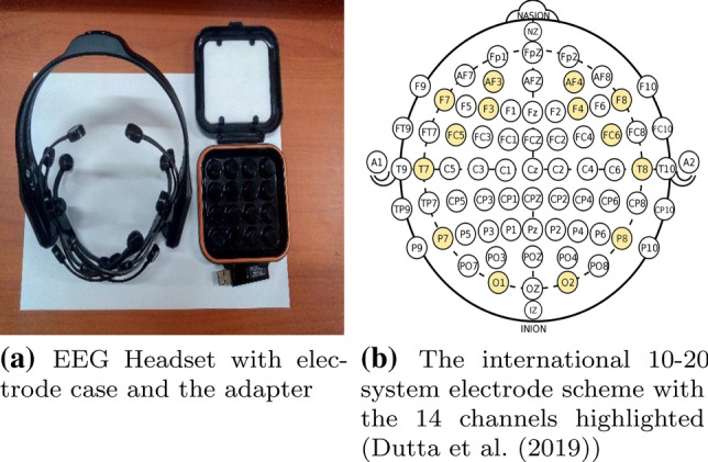
Emotiv Epoc+ 14-channel headset details
Fig. 2.
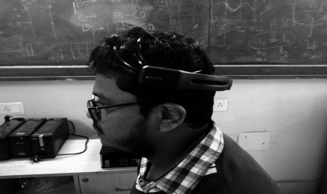
Subject wearing the Emotiv headset (Dutta et al. 2019)
Test subjects
Fifteen subjects contributed for the EEG sample data collection experiment for utilisation in the study reported in this work. Data is collected based on our proposed protocol fully abiding by NIT Rourkela, IRB guidelines. All the subjects are physically and mentally fit and provided their written consent for our proposed protocol-based experimental work depicted in this paper. The demographic information of all participants are presented in Table 1.
Table 1.
Demographic characteristics of subjects
| Variable | Values |
|---|---|
| Age (years) | 23.3 ± 2.412 |
| Gender | 14 M / 01 F |
| Education (years) | 16.7±1.159 |
Data has been presented as Mean ± SD
M : male, F : female
Procedure Implemented
External stimuli are gathered from multiple sources which further helps in the generation of various cognitive states such as EOS (Emotion Oriented State), MOS (Memory Oriented State), ROS (Relaxing Oriented State), TOS (Thinking Oriented State), SROS (Simple Regular Oriented State) and IOS (Illness Oriented State ) respectively. The corresponding environments are created using vision based stimuli as depicted through Table 2. The proposed experimental protocol is shown in Fig. 3. The protocol has six sessions corresponding to the six cognitive states (EOS, MOS, ROS, TOS, SROS, IOS) with an interval of 5–10 minutes between the sessions. Each of the sessions include four different walking speeds slow (1.5 km/h), normal (3 km/h), fast (5 km/h) and running (6.5 km/h) with video clips displayed for 15–30 seconds between the trials pertaining to different cognitive states. Subjects are advised to walk on the treadmill in all the four specified speed levels wearing the Emotiv EPOC+ 14 channel headset in the novel event driven environment. To facilitate proper data collection, the subjects are advised to take some rest before the start of the experiment and focus on the external stimuli. The interval between the trial sessions (5–10 mins) allows the participants to relax during the experiment. Also, such intervals helped in avoiding any kind of influence of one speed over the other which might attract wrong results. All sessions of the protocol lasted for 46 minutes approximately. EEG signals corresponding to the different cognitive states are collected. Also the novel environment set up involves dim-lighted conditions to rule out any kind of visual disturbance(s).
Table 2.
Generation of cognitive states for walking speeds of 1.5, 3, 5 and 6.5 km/h
| EOS | TOS |
|---|---|
| Geneva affective pictures database (GAPED) | Logical Puzzles, Crosswords |
| MOS | SROS |
| Remembering any kind of pattern such as VIBGYOR colours, Shapes, Number, etc. | Any kind of stimuli |
| ROS | IOS |
| Pictures of sea beach, puppy playing, GAPED database | Pictures of Butchery, mass murder, GAPED database. |
Fig. 3.
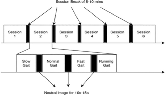
Proposed EEG data collection protocol
Workflow adopted
The proposed workflow is explained in Fig. 4. Raw EEG data is collected from fifteen subjects as described previously in section "Acquisition of EEG data". The dataset undergoes pre-processing as explained in the following section:
Fig. 4.

Proposed workflow
Pre-processing of EEG data
The raw EEG signals are depicted in Fig. 5a. An unwanted phenomenon known as DC offset occurs due to the electrode-tissue interface. The value of DC bias varies from 20 mV to 50 mV which amounts to almost 1000 times larger than the original signal. Thus, DC bias removal is a pre-essential necessity and is hence applied on the raw EEG data by subtracting the mean from each of the channels respectively. It is found that on removal of the DC Bias, the magnitude of the EEG signals decreases by large scale. The dataset undergoes pre processing using Fast Fourier Transform (FFT) and bandpass filtering respectively. Fast Fourier Transform is used to convert EEG data from the original time domain to the frequency domain representation. The signals in the background are obliterated with the application of a first order high-pass filter (cutoff frequency is 0.16 HZ). Thus, the obtained signals are clearer with improved accuracies and reduced levels of noise. Only alpha (8–13 Hz) and beta (13–30 Hz) signals are used for our analysis. Thus, band pass filtering is applied and the frequencies with values less than 8 Hz and greater than 30 Hz are removed. Hence, for each of the channel, the values other than the range of (8–30 Hz) gets nullified. Figure 5b represents the refined signals after the application of FFT and band pass filtering. During the process of collection of EEG signals, certain phenomenon such as eye blinking, visual distractions, and so on act as artifacts as they contribute to the signals coming from non-neural locations. Hence, Independent Component Analysis (ICA) technique is implemented to remove such unwanted artifacts. Because of the restrictions in the size of the data obtained and processing capabilities of the hardware, the most contributing features are only considered. Since, the EEG signals are assumed to be linear mixtures of artifactual sources, application of ICA technique further minimizes the statistical dependency of the components of the EEG signal. Removing artifacts and recovering the underlying sources by segregating the mixed signals into a series of subcomponents increases the quality of the datasets. Thus, ICA technique paired with mutual information metric additionally helps in selecting the most contributing channels amongst the 14 channels. Mutual information is a method which measures the dependencies present between two variables. It is defined as follows:
| 1 |
where D is a set of feature vectors, E denotes a set of class labels, p(d) and p(e) are the marginal probability functions of d and e and
Fig. 5.

EEG signals
p(d,e) is the joint probability functions of d and e For each channel, we derive 14 independent components (IC’s). Hence a total of 14*14 components. Mutual information of each component is then calculated with each of the other components. The least 8 mutually independent components are the most independent. The minimum 8 of the average of IC’s fetches us the most contributing channels. Finally, we take the data of the 8 most independent and contributing channels for further analysis. Out of the 8 most independent channels the amplitude spectrum of channel F8 (one among the 8 channels) is shown Fig. 6a, b on the basis of the different speeds of walking from two different subjects for SROS state. The movement artifacts showcase an increase in the patterns with increase in the speed. Also variations in the movement artifact are seen with change in the electrode locations. After analyzing the power spectra shown in the same figure it is observed that the components of the movement artifact are clearly distinguishable as non-neural despite their neural locations.
Fig. 6.

Cortical component spectrum of channel F8 for SROS state
Feature extraction strategies used in this work are DWT, MFCC (Dutta et al. 2019) and GTCC (novel proposed technique for EEG signals). FDR and logistic regression strategies are applied on them for analyzing the best features. At the end, deep learning and machine learning techniques are used to classify human cognitive states with promising results.
Feature extraction algorithms
Feature extraction techniques such as Mel Frequency Cepstrum Coefficients (MFCC), Gammatone Cepstral Coefficients (GTCC), Discrete Wavelet Transform (DWT) are applied on the pre-processed EEG signals to extract the corresponding features for classifying the mental states. Also, a proposed 1D-CNN deep learning model is used to extract novel features from GTCC MFCC ensemble feature space.
DWT
Analysis of wavelets involves the reconstruction of a signal wave as a linear combination of wavelet functions weighted by wavelet coefficients. The DWT coefficients are generally obtained with the help of wavelet and scaling functions. Both highpass and lowpass filters form an integral part of the entire process. Initially, signal S[m] is fed as input to a highpass filter H[m] and a lowpass filter L[m]. Thus, the original signal is divided into two components now. Fifty percent of the samples can be spurned post filtering as per Nyquist’s theorem. The signal’s maximum frequency is now reduced from f to f/2 Hz showing that the original signal is subsampled by a factor of 2. It is represented in Eqs. 2 and 3, where and are the outputs of the highpass and lowpass filters. The DWT coefficient matrix thus found utilizes the Morse wavelet as the main wavelet. A symmetry parameter of 3 and a time-bandwidth product of 60 are the applied parameters.
| 2 |
| 3 |
MFCC
The logarithm of power spectrum of a signal undergoes a Fourier transform and generates an output. The output thus generated is known as a Cepstrum. The sampling rate of the EEG signals acquired in our work is 128 Hz. Thus, Mel-frequency cepstrum is generated with a sampling rate of 128 Hz. To achieve that, the first step involves the slicing of the entire spectrum into windows. Hamming windowing technique is used with as many as that is 385(in our case) samples inside each single window. Approximately 256 () are the overlapping samples considered between adjacent windows. Hamming window is calculated using Eq. 4.
| 4 |
where X : number of samples.
Eq. 5 is used to wrap the signal’s spectrum into Mel scale.
| 5 |
where freq : physical frequency in Hertz, mel(freq) : frequency in mel-scale.
The next step involves obtaining the power spectrum (i.e. square of mel-spectrum) . The mathematical formulation for the same is given in Eq. 6.
| 6 |
At the end, Discrete Cosine Transform (DCT) technique is enforced upon the obtained Mel frequency coefficients. The outcome is a collection of cepstral coefficients. Also, the non-linear rectification process prior to DCT computation involves a log operation, which gives signals in cepstral domain. Hence, MFCC features are obtained by performing Inverse Discrete Cosine Transform (IDCT) as per Eq. 7.
| 7 |
where : MFCC, u : number of MFCCs < N, N : number of mel-filters.
GTCC
The proposed novel feature extraction technique Gammatone Cepstral Coefficients (GTCC) also known as Gammatone Frequency Cepstral Coefficients (GFCC) for ambulatory EEG signals has almost same computational complexity as that of MFCC feature extraction method but with superior performance. The pre-processed EEG signals are passed through a Gammatone filter bank followed by windowing analogous to MFCC scheme. Thus, a sub-band spectrum is obtained, wherein each of the sub-band’s energy is represented by . The non-linear rectification process here involves cubic root operation on the power spectrum obtained followed by DCT to obtain the GTCC cepstral coefficients. GTCC is formulated as given in Eq. 8.
| 8 |
where : GTCC, : energy of the signal in the sub-band of the spectrum, G : number of Gammatone filters, K : number of GTCC cepstral coefficients.
Spatial distribution of the extracted features (GTCC, MFCC and DWT) for the EOS class are depicted in Fig. 8. After the features are extracted, all the combination feature sets (GTCC + MFCC, GTCC + DWT and MFCC + DWT) for our work are tested and analysed further. Section "Feature importance analysis" deals with the significance tests for the extracted features from our novel ambulatory EEG dataset. It is seen that our proposed GTCC features for the EEG signals has the highest discriminative ability as per the FDR and the LR scores obtained when compared to MFCC or DWT features. Following which it is also visible in section "Feature importance analysis" that out af all the ensemble feature spaces proposed, GTCC−MFCC or GTCC MFCC ensemble feature sets are the most relevant based on the feature importance scores obtained. Thus, GTCC + MFCC feature sets are then fed into a proposed 1D-CNN model and novel EEG features are automatically extracted. The proposed 1D-CNN architecture is explained hereby.
Fig. 8.

Extracted features’ distribution for EOS class
Proposed 1D-CNN framework
(GTCC MFCC ) ensemble features extracted are passed through proposed 1D-CNN model for automatic extraction of novel features for ambulatory EEG dataset. Our 1D-CNN model consists of 5 convolutional layers, 3 max-pooling layers and 3 dense or fully-connected layers. The convolutional layers consists of kernels which slide across the input. The ouput formed from this layer is a feature map. For inculcating knowledge about the feature-learning process of the proposed CNN architecture, feature maps are produced. These maps are the outcomes obtained, when filters are applied to a sample segment at every convolution layer. Feature map values are calculated as per the following formula:
| 9 |
where the input tensor is denoted by m and the kernel by k. The indices of the rows and columns of the resultant matrix is represented as i and j respectively. An input matrix of the ensemble feature space bearing dimensions 240 13 is fed into the first convolutional layer. The output of the convolutional layer is obtained as an activation map. Relevant features are extracted from the input matrix on application to the convolution layer due to the filters. The activation function used is rectified linear unit (ReLU) which imparts non-linearity to the network architecture. Pooling is done for sole purpose of reducing the size of the tensor which further reduces overfitting. The number of output neurons are reduced in the max-pooling layer as it selects only the maximum value in the feature map and average pooling computes average of the values in a window. Pool size of the max-pooling layer is set to 3. Max-pooling is done on the entire feature map. Strides is the term used to describe the count of pixels shifts over the input tensor. For, the first convolution layer the stride is 4. The strides is fixed at 1 and 2 for the rest 4 convolutional layers and max-pooling layers respectively. The first max-pooling layer of the 1D-CNN architecture generates 96 features. For stabilization of the learning, batch normalization normalizes the input to each unit, which then possesses zero mean and unit variance. This substantially aids in dealing with training issues that are raised because of bad initialization and helps gradient flow in deeper models. It is essential to obtain deep generators to initiate learning, preventing the generator from collapsing all samples to a single point. The last three convolution layers are directly connected. After completing all the layers of convolution and pooling, the tensor is flattened to get a 200 unit vector and 3 dense layers is applied to it. The final output of the CNN model is essentially based on weights and biases of the previous layers in the structure. In each dense layer, there is a dropout of 0.2 and activation function is ReLU for the first two layers . The third and the last dense layer is the regularly deeply connected neural network structure with softmax activation function which predicts the class of the EEG signal. It is also referred usually as the output layer. For our case there are 6 class labels, which is the number of cognitive states in the EEG signals and hence the output. Compilation is done using the adam optimizer to find the accuracy of the model. It is a stochastic gradient method which is based on adaptive estimation of first-order and second-order moments. Figure 7 demonstrates the proposed 1D-CNN architecture.
Fig. 7.

Proposed 1D CNN architecture
Feature importance analysis
Performances exhibited by the classification models play a vital role in various pattern recognition and machine learning problems. To aid to these, feature selection procedure act as an integral part. All features extracted are not always relevant for classification or regression tasks, and hence some of the features are redundant. These irrelevant features further reduce classification performances. In order to improve classification accuracies and to reduce computational cost of the classifiers, FDR technique is applied to calculate robustness and suitability of the extracted features based on the scores obtained. FDR is calculated using Eqs. 10 and 11.
| 10 |
| 11 |
where X is a transformation matrix, is between-class scatter matrix and is within-class scatter matrix. Another technique used in this work to test the importance of each feature relative to one other for making the predictions, is logistic regression. Mathematical formulation for logistic regression is given in equations below:
| 12 |
where & : Predictors of the logistic model, : Probability of an event , X: is a binary response variable, k : log-odds, r : base of the algorithm, : Parameters of the specific model
Assumption : A linear relationship exists between the log-odds of the event that and the predictor variables.
The feature significance scores obtained by FDR and logistic regression techniques are illustrated in Fig. 9a, b. The CNN-Feature in Fig. 9a, b denotes the GTCC + MFCC + CNN features only. It is distinctly visible that GTCC features are highly contributing as compared to MFCC and DWT, wherein DWT being the least for our work. Furthermore, the ensemble GTCC + MFCC feature set and proposed GTCC + MFCC + CNN features extracted are highly discriminative and contributing as compared to all the features and give comparable results. We do not consider for further analysis the combined GTCC + MFCC + DWT feature space as they are not so significant with respect to the ensemble feature space or GTCC + MFCC + CNN features as can be seen in the feature importance score plots. Also processing GTCC + MFCC + DWT feature space makes it highly computationally intensive. The better values of GTCC features can basically be attributed to certain factors. GTCC’s equivalent rectangular bandwidth (ERB) scale has finer resolution at low frequencies as compared to MFCC’s mel scale. The other major factor is the non-linear rectification process. This process in GTCC involves cubic root operation which provisions the features with more robustness than log operation in the case of MFCC. The cubic root operation also helps in retaining a significant amount of spectral information which is otherwise not encoded by the log operation in case of MFCC. Also, the entire process for DWT becomes computationally intensive for intricate analysis. Again, sometimes it so happens during denoising, that the signals are not represented aptly with satiating accuracies in the frequency domain by the DWT coefficients and hence the results.
Fig. 9.

Feature importance score plots
Classification models
The geometry of the feature vectors fed as inputs generally influence the selection of classifiers. Also, as a single classification model cannot be particularly guaranteed to be appropriate for a specific dataset, we apply different machine learning and deep learning classifiers to classify the six cognitive states. The classifiers in this work are trained and tested in (70:30) pattern and the validation procedure used is shuffled K-fold cross validation. The classifiers used in this work are described briefly in the following subsections.
Probabilistic neural network
A popular multilayered feed-forward neural network for classification and pattern recognition problems is Probabilistic Neural Network (PNN). PNN algorithm functions by using two parameters : Parzen window & a non-parametric function to estimate the parent probability distribution function (PDF) of each class. Largest vote technique is used for final prediction and classification.
Linear discriminant analysis
Linear Discriminant A-nalysis or LDA is one of the widely used techniques in machine learning problems for dimensionality reduction and pattern classification problems as well. LDA is highly suitable for multi-class classification. It’s functionality begins by initially calculating the class separability and hence calculating the between-class variance. It is followed by calculating the distance between the mean and sample of each class known as within-class variance and finally constructing the lower-dimensional space which results in the maximization of between-class variance and minimization of within-class variance. LDA’s feature selection property is also dealt with. The ratio also known as Fisher’s criterion is as expressed in Eqs. 10 and 11 in section "Feature importance analysis". The LDA classifier works by basically using two assumptions that the variables follow a Gaussian distribution and each attribute has the same variance. LDA models use Bayes’ Theorem for probability estimation and hence classification.
Decision tree
The classifier works by generating a decision tree. Each vertex or node in the tree is a specification of an attribute test, whereas each edge or a branch descending from that node corresponds to the possible attribute values. The leaf nodes represent the class labels. The decision tree thus operates in a top-down manner, by selecting test condition of an attribute at each step that splits the records in the best case. The splitting is based on a number of criteria such as Gini index, entropy and so on.
Random forest
Random Forest classifiers involve a large number of decision trees for classification and are thus based on ensemble learning methods. Each decision tree in random forest spits out the prediction of a class. The class with the maximum number of votes turns out to be the prediction outcome of the model. The problem of overfitting a model is generally reduced. Low correlation between decision tree models is the underlying principle to successful and superior classification.
Multi-class support vector machine
Support-vector machines (SVM)s are supervised learning models for classifying multi-dimensional data in machine learning. The associated learning algorithms aids in performing both linear & a non-linear classification, by making use of the kernel function e.g. a radial basis function. The inputs are mapped into high dimensional feature spaces. Multiclass SVM assigns labels to instances, the labels which are drawn from a finite set of several elements. Thus a single multi class problem is reduced into multiple binary classification problems. The support vector machines mainly initiate the construction of a hyperplane or set of hyperplanes in a high-dimensional feature space for classification, regression. More is the margin, the lesser is the error of the classifier. Hence, the hyperplane that possesses the largest separation to the closest data point of any class, attains a comparatively good separation. In higher-dimensional spaces, hyperplanes are set of data points whose dot product with a vector in that space does not vary. The vectors are set of orthogonal vectors that define a hyperplane.
1D convolutional neural network
The 1D-CNN model described in section "Feature extraction algorithms" for feature extraction is used for classification purpose as well. It is mainly used to evaluate the accuracies achieved on passing the GTCC, GTCC + MFCC and GTCC + MFCC + CNN features separately through it. Also, it is one of the ground truths for validation of superior performances of our proposed model which involves the passing of novel GTCC , GTCC +MFCC and GTCC + MFCC + CNN features separately through the proposed 1D DCGAN classifier. Detailed explanations and discussions are given in section "Comparative analysis with state-of-the-art methods".
Proposed 1D deep convolutional generative adversarial network
DCGAN is the most popular and rewarding design for GAN. It is formed using two models—generator and discriminator. The generator performs the work of creating fake signals that resemble the training vector. The task of the discriminator is to determine whether the vector is fake or real. The generator and the discriminator work together in such a way that the generator attempts to reduce the Minimax loss function whereas the discriminator attempts to maximize the value of the loss. The Minimax loss function is as follows:
| 13 |
where T(a) represents the discriminator’s estimate of the probability that data instance a is real, denotes the expected value over all real data instances, H(b) is the generator’s output when additional noise b is combined with the real dataset, T(H(b)) is the estimate of the probability of fakeness of the dataset by the discriminator, is the expected value over all random inputs to the generator.
The derivation of Eq. 13 comes from the cross-entropy between the real and fake dataset from the generator. The generator can’t affect the term directly in the function. Hence, it minimizes the loss i.e. . The discriminator is composed of convolution layers without max-pooling or fully connected layers. The DCGAN further uses convolutional stride and transposed convolution for down sampling which takes place in the discriminator and up sampling which takes place in the generator. DCGAN administers the competition between two networks to establish a dynamic balance for learning the statistical distribution of the required output. The parameters of the proposed architecture of this specific deep learning model in our work, undergo optimization through the changing and tuning of it’s variants such as the number of layers, filters in the various layers, stride windows, input and the output vector lengths and so on. Hence trying out different possibilities, the parameters flaunting the best performance are incorporated into the 1D DCGAN architecture for that particular feature. All the proposed features of our work are passed through the proposed 1D DCGAN classifier and the performance metrics are discussed further in section "Comparative analysis with state-of-the-art methods". Out of all the proposed features, the ensemble (GTCC+MFCC) feature space fetches the maximum accuracy. Hence, the proposed 1D DCGAN architecture explained in this section and depicted in Fig. 10a, b is for the ensemble (GTCC+MFCC) feature space.
- Generator As shown in Fig. 10a, a six-layer network with a dense layer, 3 convolutional layers, batch normalization and activation layers is proposed in our study. The presence of convolutional layers and implementation of up-sampling ensures that the output is consistent with the original training dataset. The kernel size is 3 in each of the convolution layers of the generator. Kernels are the filters with the help of which the receptive field of a convolutional network is known. The activation function used is Leaky ReLU in all the layers except the last layer where tanh activation function is used. The working of the generator is described as follows:
- Working principle The dense layer at the beginning of the model feeds the input array to all the neurons, which further produces one output for each of the neurons and hence, produces an output of 14400 in dimension. It is further reshaped to form a matrix of size 60*240. The matrix is upsampled to a size of 120*240 which increases the resolution of the dataset and reduces the error. The matrix is fed to the first convolution layer, batch normalization and activation layers respectively. The activation function introduces non-linearity to the matrix. The dataset is further passed through the second layer of convolution, batch normalization and activation. The third convolution layer produces an output matrix of size 240*13. Activation layer is applied finally to get an output matrix.The model summary for the generator of the proposed 1D DCGAN classifier is represented in Table 3.
- Discriminator The network architecture as illustrated in Fig. 10b consists of 4 convolutional layers, 2 dense layers, zero-padding, batch normalization and activation layers. The stride size and kernel size is both 2 in each of the convolution layers. The slope of the leak in the Leaky ReLU is 0.2 and batch-normalization has a momentum of 0.8. The activation function Leaky ReLU speeds up the training process and it follows the function of where & denotes the slope of the activation function. The mean activation which is closer to 0 makes it work faster. The discriminator focuses on predicting the authenticity of the generated data depending on it’s realness or fakeness. The working of the discriminator is explained as follows:
- Working principle The discriminator is first fed with an input of size . The first convolution layer transforms the input matrix to a dimension of . While lowering the size of the dataset over the convolution layer, the features are extracted without losing its characteristics. The second convolution layer converts the shape to . Padding is carried out so that a layer of zeros is added to the input matrix, transforming it into a shape of . The third convolution layer transforms the matrix dimension to . The last convolution layer produces an output of . A flattening layer is used at the end whose output of shape 4096. Finally, the dense layer gives the output of the classification of cognitive states by learning features on the basis of the previous layer producing an output of size 4097 in dimension. The model summary for the discriminator of the proposed 1D DCGAN classifier is represented in Table 4.
Fig. 10.

Proposed 1D DCGAN generator architecture for GTCC+MFCC features
Table 3.
Model summary for the generator
| Layer (type) | Output shape | Param # |
|---|---|---|
| dense_1 | (None, 14400) | 1,022,400 |
| reshape_1 | (None, 60, 240) | 0 |
| up_sampling1d_1 | (None, 120, 240) | 0 |
| conv1d_1 | (None, 120, 240) | 173,040 |
| batch_normalization_1 | (None, 120, 240) | 960 |
| activation_1 | (None, 120, 240) | 0 |
| up_sampling1d_2 | (None, 240, 240) | 0 |
| conv1d_2 | (None, 240, 120) | 86,520 |
| batch_normalization_2 | (None, 240, 120) | 480 |
| activation_2 | (None, 240, 120) | 0 |
| conv1d_3 | (None, 240, 13) | 4693 |
| activation_3 | (None, 240, 13) | 0 |
Table 4.
Model summary for the discriminator
| Layer (type) | Output shape | Param # |
|---|---|---|
| conv1d_4 | (None, 120, 32) | 864 |
| leaky_re_lu_1 | (None, 120, 32) | 0 |
| dropout_1 | (None, 120, 32) | 0 |
| conv1d_5 | (None, 60, 64) | 4160 |
| zero_padding1d_1 | (None, 62, 64) | 0 |
| batch_normalization_3 | (None, 62, 64) | 256 |
| leaky_re_lu_2 | (None, 62, 64) | 0 |
| dropout_2 | (None, 62, 64) | 0 |
| conv1d_6 | (None, 31, 128) | 16,512 |
| batch_normalization_4 | (None, 31, 128) | 512 |
| leaky_re_lu_3 | (None, 31, 128) | 0 |
| dropout_3 | (None, 31, 128) | 0 |
| conv1d_7 | (None, 16, 256) | 65,792 |
| batch_normalization_5 | (None, 16, 256) | 1024 |
| leaky_re_lu_4 | (None, 16, 256) | 0 |
| dropout_4 | (None, 16, 256) | 0 |
| flatten_1 | (None, 4096) | 0 |
| dense_2 | (None, 1) | 4097 |
Thus, there are 3 phases while training the dataset using DCGAN approach:
Phase 1: In the first phase, the entire training data is used to train the discriminator. The discriminator is treated as a standalone classifier. The generator is kept idle during this period.
Phase 2: After the first phase is completed, the generator is trained by taking small amount of noise into account which makes multiple fake data from it. The job of the generator is to increase the testing sample by creating more fake datasets.
Phase 3: All of the training data which include the real data as well as the data produced by the generator is utilized by the discriminator during training. It determines whether the data fed into, is fake or real.
On the basis of output of the discriminator, the generator again creates new data from which it is then sent to the discriminator for its training. Hence, the proposed 1D DCGAN model is able to discriminate between very close states. One of the essential hyper-parameters for the proposed 1D DCGAN classifier is the optimizer used in the discriminator. Four optimizers namely Adam, AdaGrad, AdaDelta and RmsProp are tested with. Figure 11 depicts the accuracy versus epoch curve for all the optimizers. It is clearly seen that the Adam optimizer fetches the best validation accuracy after training. Thus, Adam optimizer with a learning rate of and is used.
Fig. 11.

Validation accuracy versus epoch curve for the optimizers used in 1D DCGAN discriminator
Another important hyper-parameter for the 1D DCGAN model is using certain regularisation techniques such as dropout or early stopping to prevent over-fitting. Dropout generally refers to dropping out units in a neural network. It simply involves ignoring units during the training phase of the model. Another technique to prevent over-fitting is early stopping. It basically stops training when the generalization error and hence the validation accuracy begins to degrade (Sjöberg and Ljung 1995). Time and again dropout method has reduced overfitting in deep neural networks with large number of parameters (Krizhevsky et al. 2017) as well as in neuroimaging application (Plis et al. 2014). But for early stopping, the model gets prevented from over-training i.e. a lot of our training data would not be used. This is definitely not recommended for our work in which we essentially have 6 mental states and hence a large network. Thus, we use dropout in the hidden layers with a probability of 0.25. This means, in each weight updation cycle, 25% neurons would be dropped. This technique is appropriate for our context as is visible from Figs. 11 and 27. In both the graphs, initially the validation accuracy for 1D DCGAN classifier, increases for certain epochs after which it becomes constant. As the validation accuracy does not degrade, our model is not prone to much over-fitting and hence dropout regularisation technique is rightfully executed.
Fig. 27.
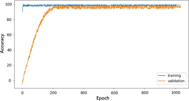
Accuracy versus epoch curve for 1000 epochs for feature space and 1D DCGAN model
Results analysis and discussion
After the EEG signals are pre-processed, feature extraction and classification models are applied on the processed data to classify the six cognitive states in our work. The entire data used for extensive analysis eventually are from the eight most contributing channels obtained by the sequential steps followed in pre-processing. DWT, MFCC and GTCC techniques are applied on our dataset generated in our novel event driven environment and hence the corresponding features are obtained. Following which, FDR and logistic regression techniques are applied, inferring that irrespective of the feature selection techniques used. Hence GTCC is the preferred feature for further classification. The geometry of the feature vectors fed as inputs generally influence the selection of classifiers. Also, as no single classification model can be guaranteed to be appropriate for a particular dataset, we apply different machine learning classifiers to classify the six cognitive states. All the individual features extracted are flattened into a 1D vector of same dimensions and then fed into the machine learning classifiers. The classifiers in our work are trained and tested in (70:30) pattern and the validation procedure used is shuffled K-fold cross validation. After the features are extracted, ensemble feature spaces are proposed in this work for the ambulatory EEG data collected in our novel experimental setup. The ensemble feature spaces are basically GTCC+MFCC, GTCC+DWT and MFCC+DWT respectively. Thus, for multi feature analysis, suppose for GTCC+MFCC feature space, GTCC and MFCC feature sets are passed together through the machine learning classifiers after each of the feature sets are flattened into 1D vectors. Hence, the ensemble feature space. Similar process is followed for all the combinations and it is found that the FDR and LR scores for them are in this order : . Thus, GTCC+MFCC is used for further processes as they are highly discriminative. Finally, the last novel task is hereby discussed. GTCC+MFCC feature sets are passed through the proposed 1D CNN model and features are automatically extracted. Also it is found that the FDR and LR scores of the GTCC+MFCC+CNN features GTCC+MFCC features and hence are considered highly contributing. These features are then passed through the proposed 1D DCGAN model. It is seen that with reduced dimensions, these features generate comparable accuracies to the GTCC+MFCC feature space, when passed through DCGAN classifier and also the machine learning classifiers. However, the 1D DCGAN classifier performs much better for all the proposed features than the machine learning classifiers.
Performance evaluation of the individual features
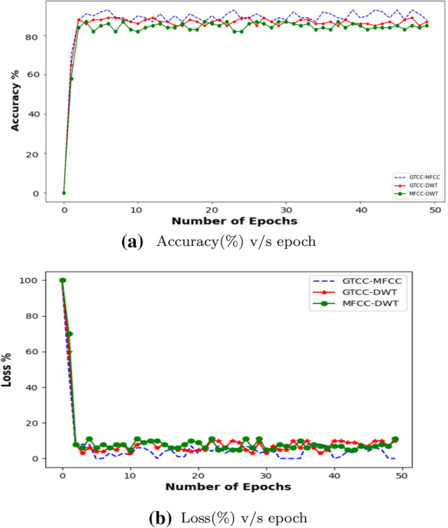
Table 5 shows different statistical measures for the entire group of feature extraction techniques and the machine learning classification models used in this research work. It is inferred from the table that P-NN is one of the strongest classifiers to classify the six mental states with our novel feature extraction technique i.e. GTCC. This is well confirming with the fact that GTCC features are superior as compared to MFCC features. Further more, the fact that, MFCC feature extraction technique is highly suited and gives promising results for ambulatory EEG signal analysis has been proved in our previous work Dutta et al. (2019). Figure 12a shows accuracy plot for training data versus epochs in PNN clearly stating the fact that accuracy is more for GTCC than MFCC and DWT in almost each epoch. Loss plot (Fig. 12b) of the PNN model depicts that the classifier fits data considerably better for GTCC feature than the other extracted features.
Table 5.
Statistical measures for different classifiers along with the feature extraction methods
| GTCC | MFCC | DWT | ||||||||||||||||||
|---|---|---|---|---|---|---|---|---|---|---|---|---|---|---|---|---|---|---|---|---|
| EOS | IOS | MOS | ROS | SROS | TOS | EOS | IOS | MOS | ROS | SROS | TOS | EOS | IOS | MOS | ROS | SROS | TOS | |||
| PNN | ACCURACY : 91.14% | ACCURACY : 89.50% | ACCURACY : 79.46% | |||||||||||||||||
| Precision | 0.912 | 0.921 | 0.917 | 0.901 | 0.913 | 0.922 | 0.901 | 0.898 | 0.900 | 0.902 | 0.889 | 0.903 | 0.870 | 0.801 | 0.798 | 0.776 | 0.756 | 0.823 | ||
| Recall | 0.914 | 0.920 | 0.902 | 0.899 | 0.901 | 0.905 | 0.876 | 0.889 | 0.899 | 0.901 | 0.902 | 0.888 | 0.835 | 0.802 | 0.778 | 0.767 | 0.762 | 0.821 | ||
| F-Measure | 0.917 | 0.918 | 0.904 | 0.901 | 0.919 | 0.920 | 0.901 | 0.910 | 0.872 | 0.882 | 0.896 | 0.907 | 0.801 | 0.791 | 0.778 | 0.761 | 0.763 | 0.820 | ||
| LDA | ACCURACY : 84.77% | ACCURACY : 83.67% | ACCURACY : 79.11% | |||||||||||||||||
| Precision | 0.858 | 0.828 | 0.834 | 0.798 | 0.897 | 0.835 | 0.841 | 0.837 | 0.812 | 0.861 | 0.867 | 0.832 | 0.797 | 0.782 | 0.767 | 0.801 | 0.799 | 0.786 | ||
| Recall | 0.821 | 0.827 | 0.887 | 0.867 | 0.851 | 0.849 | 0.828 | 0.861 | 0.860 | 0.851 | 0.811 | 0.808 | 0.791 | 0.792 | 0.788 | 0.771 | 0.806 | 0.801 | ||
| F-Measure | 0.817 | 0.812 | 0.881 | 0.895 | 0.816 | 0.886 | 0.847 | 0.840 | 0.831 | 0.828 | 0.832 | 0.814 | 0.799 | 0.794 | 0.801 | 0.800 | 0.789 | 0.777 | ||
| RF | ACCURACY : 81.48% | ACCURACY : 78.35% | ACCURACY : 70.37% | |||||||||||||||||
| Precision | 0.828 | 0.811 | 0.809 | 0.831 | 0.827 | 0.809 | 0.781 | 0.799 | 0.797 | 0.791 | 0.801 | 0.776 | 0.698 | 0.707 | 0.734 | 0.667 | 0.680 | 0.771 | ||
| Recall | 0.818 | 0.821 | 0.810 | 0.819 | 0.799 | 0.800 | 0.768 | 0.799 | 0.799 | 0.790 | 0.777 | 0.784 | 0.771 | 0.701 | 0.712 | 0.682 | 0.680 | 0.728 | ||
| F-Measure | 0.829 | 0.831 | 0.801 | 0.807 | 0.798 | 0.820 | 0.758 | 0.762 | 0.792 | 0.782 | 0.777 | 0.771 | 0.714 | 0.675 | 0.668 | 0.667 | 0.704 | 0.709 | ||
| DT | ACCURACY : 78.62% | ACCURACY : 74.89% | ACCURACY : 68.03% | |||||||||||||||||
| Precision | 0.781 | 0.772 | 0.797 | 0.801 | 0.800 | 0.768 | 0.747 | 0.748 | 0.743 | 0.767 | 0.724 | 0.782 | 0.681 | 0.667 | 0.707 | 0.660 | 0.648 | 0.739 | ||
| Recall | 0.812 | 0.788 | 0.777 | 0.769 | 0.801 | 0.779 | 0.732 | 0.751 | 0.757 | 0.741 | 0.717 | 0.738 | 0.729 | 0.689 | 0.677 | 0.698 | 0.634 | 0.681 | ||
| F-Measure | 0.788 | 0.781 | 0.799 | 0.765 | 0.775 | 0.799 | 0.771 | 0.737 | 0.766 | 0.729 | 0.781 | 0.750 | 0.688 | 0.645 | 0.657 | 0.689 | 0.682 | 0.676 | ||
| MCSVM | ACCURACY : 77.03% | ACCURACY : 73.25% | ACCURACY : 66.49% | |||||||||||||||||
| Precision | 0.777 | 0.789 | 0.761 | 0.766 | 0.769 | 0.739 | 0.739 | 0.744 | 0.729 | 0.717 | 0.767 | 0.720 | 0.646 | 0.637 | 0.601 | 0.689 | 0.647 | 0.681 | ||
| Recall | 0.798 | 0.801 | 0.723 | 0.776 | 0.772 | 0.789 | 0.749 | 0.738 | 0.724 | 0.757 | 0.760 | 0.712 | 0.648 | 0.666 | 0.678 | 0.669 | 0.672 | 0.680 | ||
| F-Measure | 0.770 | 0.759 | 0.779 | 0.764 | 0.778 | 0.757 | 0.708 | 0.702 | 0.732 | 0.728 | 0.741 | 0.718 | 0.679 | 0.682 | 0.668 | 0.675 | 0.671 | 0.680 | ||
Bold values indicates the best accuracies obtained by our proposed techniques and are hence significant
Fig. 12.

Plots for individual features and PNN classifier
Receiver Operating Characteristic (ROC) curve is a plot of true positive rate (TPR) against false positive rate (FPR) at different thresolds for any classification model. The training, testing, validation and overall ROC curves shown in Fig. 13a–d demonstrate the analytical ability of a P-NN classifier using GTCC for assessment of classification quality at various stages. Also it is inferred that the training, testing roc curves boast of better performance than the validation process as the curves are located near the top left corner of ROC.
Fig. 13.

ROC curves (one versus all classes) for PNN classifier with GTCC features
The error histogram plot (Fig. 14) of the PNN classifier for training, testing and validation steps clearly indicate that within a reasonable range the data fitting errors are distributed around the zero error. Error measures between obtained output and the target output for the training, testing & validation steps for each class for PNN classifier utilizing GTCC features is shown in the cross entropy performance graph (Fig. 15). Also it is visible from Fig. 15 that the best validation performance is 0.218 at epoch 14.
Fig. 14.

Error histogram plot for P-NN classifier with GTCC
Fig. 15.

Cross entropy performance plot for P-NN classifier with GTCC
Performance evaluation of the ensemble feature space and proposed GTCC+MFCC+CNN features
Table 6 shows different statistical measures for the entire group of ensmeble feature sets with the machine learning classification models used in this research work. It is again inferred from the table that P-NN is the strongest classifier with our novel ensemble feature set i.e. GTCC + MFCC. When compared to the individual feature analysis carried out in section "Performance evaluation of the individual features", all the combined feature sets generate better accuracies with the same classifiers. This is due to the fact that with mixture of features the diversity increases and hence better outcomes are fetched. Figure 16a shows accuracy plot of the proposed feature spaces for training data versus epochs in PNN clearly stating the fact that accuracy is more for GTCC + MFCC than GTCC + DWT and MFCC + DWT for each and every epoch. The loss plot (Fig. 16b) of the PNN model depicts that this classifier fits data considerably better for GTCC + MFCC features than the other extracted features.
Table 6.
Statistical measures for different classifiers along with the ensemble feature extraction methods and GTCC+MFCC+CNN features : ( GTCC-MFCC = GTCC+MFCC, GTCC-DWT = GTCC+DWT, MFCC-DWT = MFCC+DWT, GTCC-MFCC-CNN = GTCC+MFCC+CNN )
| GTCC-MFCC | GTCC-DWT | MFCC-DWT | GTCC-MFCC-CNN | ||||||||||||||||||||||
|---|---|---|---|---|---|---|---|---|---|---|---|---|---|---|---|---|---|---|---|---|---|---|---|---|---|
| EOS | IOS | MOS | ROS | SROS | TOS | EOS | IOS | MOS | ROS | SROS | TOS | EOS | IOS | MOS | ROS | SROS | TOS | EOS | IOS | MOS | ROS | SROS | TOS | ||
| PNN | ACCURACY : 94.01% | ACCURACY : 91.50% | ACCURACY : 90.96% | ACCURACY : 94.89% | |||||||||||||||||||||
| Precision | 0.942 | 0.941 | 0.937 | 0.947 | 0.933 | 0.938 | 0.911 | 0.898 | 0.910 | 0.912 | 0.909 | 0.913 | 0.910 | 0.908 | 0.909 | 0.910 | 0.911 | 0.910 | 0.949 | 0.942 | 0.938 | 0.946 | 0.938 | 0.939 | |
| Recall | 0.944 | 0.940 | 0.942 | 0.939 | 0.941 | 0.935 | 0.916 | 0.909 | 0.899 | 0.911 | 0.912 | 0.898 | 0.911 | 0.912 | 0.909 | 0.908 | 0.912 | 0.911 | 0.944 | 0.951 | 0.942 | 0.939 | 0.946 | 0.937 | |
| F-Measure | 0.947 | 0.938 | 0.944 | 0.931 | 0.939 | 0.940 | 0.910 | 0.927 | 0.932 | 0.921 | 0.916 | 0.917 | 0.911 | 0.911 | 0.908 | 0.912 | 0.913 | 0.909 | 0.946 | 0.939 | 0.944 | 0.932 | 0.941 | 0.943 | |
| LDA | ACCURACY : 92.77% | ACCURACY : 91.27% | ACCURACY : 90.11% | ACCURACY : 92.97% | |||||||||||||||||||||
| Precision | 0.928 | 0.927 | 0.930 | 0.928 | 0.926 | 0.926 | 0.912 | 0.917 | 0.908 | 0.913 | 0.912 | 0.911 | 0.907 | 0.901 | 0.897 | 0.901 | 0.899 | 0.896 | 0.929 | 0.929 | 0.932 | 0.931 | 0.931 | 0.928 | |
| Recall | 0.927 | 0.927 | 0928 | 0.926 | 0.928 | 0.927 | 0.911 | 0.913 | 0.912 | 0.912 | 0.911 | 0.912 | 0.905 | 0.902 | 0.901 | 0.902 | 0.906 | 0.901 | 0.929 | 0.929 | 0.928 | 0.926 | 0.932 | 0.928 | |
| F | 0.928 | 0.926 | 0.928 | 0.926 | 0.927 | 0.928 | 0.912 | 0.911 | 0.912 | 0.913 | 0.912 | 0.911 | 0.901 | 0.904 | 0.891 | 0.890 | 0.889 | 0.907 | 0.928 | 0.926 | 0.928 | 0.925 | 0.932 | 0.929 | |
| RF | ACCURACY : 91.48% | ACCURACY : 89.91% | ACCURACY : 88.37% | ACCURACY : 92.21% | |||||||||||||||||||||
| Precision | 0.914 | 0.913 | 0.912 | 0.915 | 0.915 | 0.914 | 0.898 | 0.899 | 0.897 | 0.896 | 0.899 | 0.899 | 0.883 | 0.884 | 0.884 | 0.884 | 0.883 | 0.884 | 0.924 | 0.923 | 0.912 | 0.925 | 0.922 | 0.921 | |
| Recall | 0.908 | 0.911 | 0.915 | 0.914 | 0.914 | 0.915 | 0.898 | 0.899 | 0.899 | 0.899 | 0.897 | 0.898 | 0.884 | 0.883 | 0.883 | 0.883 | 0.884 | 0.884 | 0.918 | 0.919 | 0.921 | 0.923 | 0.922 | 0.921 | |
| F | 0.916 | 0.912 | 0.914 | 0.915 | 0.913 | 0.914 | 0.898 | 0.899 | 0.899 | 0.899 | 0.899 | 0.899 | 0.884 | 0.883 | 0.884 | 0.883 | 0.884 | 0.883 | 0.922 | 0.909 | 0.921 | 0.923 | 0.924 | 0.923 | |
| DT | ACCURACY : 89.62% | ACCURACY : 84.89% | ACCURACY : 84.03% | ACCURACY : 90.12% | |||||||||||||||||||||
| Precision | 0.896 | 0.897 | 0.897 | 0.893 | 0.904 | 0.900 | 0.849 | 0.849 | 0.848 | 0.848 | 0.849 | 0.848 | 0.841 | 0.840 | 0.842 | 0.840 | 0.842 | 0.839 | 0.916 | 0.897 | 0.899 | 0.898 | 0.904 | 0.900 | |
| Recall | 0.892 | 0.891 | 0.907 | 0.901 | 0.901 | 0.897 | 0.849 | 0.841 | 0.857 | 0.841 | 0.860 | 0.848 | 0.840 | 0.839 | 0.842 | 0.839 | 0.841 | 0.842 | 0.899 | 0.901 | 0.907 | 0.901 | 0.901 | 0.897 | |
| F | 0.896 | 0.891 | 0.901 | 0.900 | 0.897 | 0.896 | 0.844 | 0.854 | 0.856 | 0.849 | 0.843 | 0.850 | 0.840 | 0.841 | 0.842 | 0.839 | 0.842 | 0.841 | 0.898 | 0.902 | 0.901 | 0.900 | 0.897 | 0.899 | |
| MCSVM | ACCURACY : 88.03% | ACCURACY : 83.25% | ACCURACY : 82.49% | ACCURACY : 88.01% | |||||||||||||||||||||
| Precision | 0.881 | 0.880 | 0.881 | 0.879 | 0.879 | 0.880 | 0.832 | 0.833 | 0.832 | 0.833 | 0.832 | 0.834 | 0.825 | 0.823 | 0.825 | 0.825 | 0.826 | 0.825 | 0.880 | 0.880 | 0.880 | 0.880 | 0.879 | 0.880 | |
| Recall | 0.881 | 0.879 | 0.879 | 0.880 | 0.880 | 0.880 | 0.832 | 0.833 | 0.833 | 0.832 | 0.833 | 0.832 | 0.824 | 0.825 | 0.826 | 0.824 | 0.825 | 0.824 | 0.880 | 0.879 | 0.879 | 0.880 | 0.880 | 0.880 | |
| F | 0.881 | 0.879 | 0.879 | 0.879 | 0.879 | 0.880 | 0.832 | 0.833 | 0.832 | 0.833 | 0.832 | 0.833 | 0.825 | 0.825 | 0.824 | 0.824 | 0.826 | 0.824 | 0.881 | 0.879 | 0.879 | 0.879 | 0.879 | 0.880 | |
Bold values indicates the best accuracies obtained by our proposed techniques and are hence significant
Fig. 16.
Plots for PNN classifier with the ensemble feature spaces
The error histogram plot (Fig. 17) of the PNN classifier with GTCC+MFCC feature space for training, testing and validation steps clearly indicate that again the data fitting errors are spread around the zero error within a particular range. Error measures between obtained and the target outputs for training, testing and validation steps for each class for PNN classifier with GTCC + MFCC ensemble feature space is shown in the cross entropy performance graph (Fig. 18). It is visible from Fig. 18 that the best validation performance is 0.209 at epoch 13 in this specific case.
Fig. 17.

Histogram Plot for P-NN classifier with feature space
Fig. 18.

Cross Entropy Performance Plot for P-NN classifier with feature space
The training, testing, validation and overall ROC curves depicted in Fig. 19a–d clearly manifests the analytical ability of a P-NN classifier using proposed GTCC+MFCC feature space for evaluating the classification calibre at various steps. Also it is visible that the training and testing ROC curves exhibit far better performance than the validation stage as the curves are located near the top left corner of ROC (AUC 1). Error
Fig. 19.

ROC curves (one versus all classes) for feature space with PNN classifier
After the ensemble feature spaces are analysed, GTCC + MFCC combined feature set proved out to be the best. Hence, this particular feature space is passed through the proposed 1D CNN model (Fig. 7) for automatic feature extraction. The CNN model generates almost 96 essential features for each layer. These are already discussed in the earlier sections. Table 7 gives an overview of the different possibilities tested and hence different models for acquiring the optimized parameters. Of the three models we choose the model with maximum accuracy for extracting the best features. Figure 20 presents the accuracy versus epoch curve for training and validation accuracies for the CNN model. It can be visualized that the training versus validation graph converges and hence the accuracy achieved is more than 97% as can be seen from Table 7 as well. Figure 21 shows the training and validation losses for the same model. It is hereby inferred that that the training loss is lesser than the validation loss for each epoch. Figure 22 shows the mean absolute error metrics for the training and validation of our proposed CNN model for GTCC+MFCC feature space. It is found at the end, mean absolute error for training the model is 7.07e-10 & for validation it is 1.48e-07 respectively. Hence, it is concluded that the model is trained really well as the error is very less. Also, the accuracies attained by the novel GTCC+MFCC+CNN features when passed through the machine learning classifiers is depicted in Table 6 before. It is observed that GTCC+MFCC+CNN features generate superior accuracies for all the classifiers. A maximum accuracy of 94.89% is obtained for the GTCC+MFCC+CNN features with PNN classifier. Figure 23a illustrates the test accuracy plots versus epoch for all the proposed features with the PNN classifier. Figure 23b gives the loss plots for all the proposed features with the PNN classifier. Thus, both the CNN extracted features (denoting GTCC+MFCC+CNN features in the figures) and the GTCC+MFCC ensemble feature space exhibit comparable performances but superior to the individual features. The error histogram plot (Fig. 24) of the PNN classifier with GTCC+MFCC+CNN features for training, testing and validation steps also indicate that the data fitting errors are here also spread around the zero error within a particular range like the other proposed features of our work discussed earlier. Error measures between obtained and the target outputs for training, testing & validation steps for each class for PNN classifier with the GTCC+MFCC+CNN features is shown in the cross entropy performance graph (Fig. 25). It is also seen from Fig. 25, that the best validation performance for proposed GTCC+MFCC+CNN features with the PNN classifier is 0.208 at epoch 13. The training, testing, validation and the overall ROC curves for GTCC+MFCC+CNN features with PNN classifier are shown in Fig. 26a–d. It is discernible that the training and testing ROC curves represent higher level performance than the validation stage as AUC for both almost approximate 1 unlike the latter.
Table 7.
Different models tested for proposed 1D CNN model
| Filters in | Model 1 | Model 2 | Model 3 |
|---|---|---|---|
| 1st convolution layer | 48 | 96 | 116 |
| 2nd convolution layer | 280 | 256 | 216 |
| 3rd convolution layer | 450 | 300 | 300 |
| 4th convolution layer | 450 | 300 | 300 |
| 5th convolution layer | 250 | 200 | 200 |
| 1st dense layer | 4000 | 4096 | 3500 |
| 2nd dense layer | 4000 | 3500 | 3500 |
| Accuracy | 94.23% | 97.29% | 95.19% |
Bold signifies the model chosen which gives the best accuracy
Fig. 20.

Accuracy versus epoch curve for 30 epochs for proposed CNN model
Fig. 21.

Loss versus epoch curve for 30 epochs for proposed CNN model
Fig. 22.

Mean absolute error versus epoch curve for 30 epochs for proposed CNN model for feature extraction
Fig. 23.

Plots for proposed features and PNN classifier
Fig. 24.

Error Histogram Plot for proposed features with PNN classifier
Fig. 25.

Cross Entropy Performance Plot for features with PNN classifier
Fig. 26.

ROC curves (one versus all classes) for features with PNN classifier
Peformance evaluation of the proposed features with the proposed 1D DCGAN classifier
The architecture of the proposed 1D DCGAN deep learning classification model is already discussed in section "Classification models". The proposed novel features of our work are GTCC, GTCC+MFCC & the GTCC+MFCC+CNN features respectively.
For subject-wise analysis
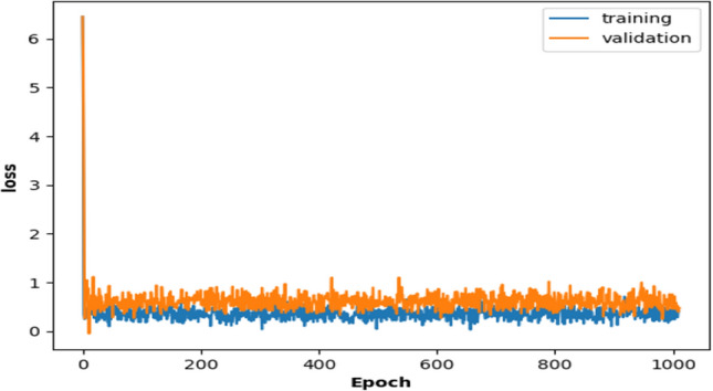
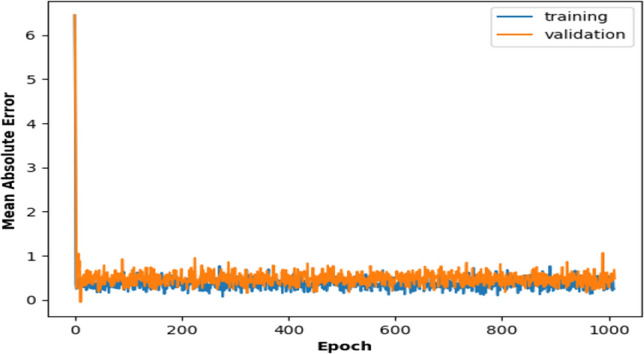
These features are passed through the 1D DCGAN model with their optimised and satiating parameters and the performance metrics are discussed in this section. In order to simply evaluate the performance of our deep learning model with the proposed features, a basic 1D CNN model is also trained with them for classification. It is found that the proposed deep learning 1D DCGAN model presents better performance than the basic CNN model. Also, the ensemble feature space GTCC + MFCC perform comparably to the GTCC + MFCC + CNN features and better than the individual proposed GTCC features for the deep learning model. The training and the validation accuracies for the DCGAN classifier with the GTCC + MFCC features is illustrated by the accuracy versus epoch curve (Fig. 27) for 1000 epochs. The curves converge really well. Table 8 gives the performance metrics for the proposed features with the basic CNN and the proposed DCGAN models respectively. The best accuracy for GTCC + MFCC feature space with the DCGAN model is 96.42% whereas for the GTCC + MFCC + CNN features is 96.14%. Hence their performances are comparable. Also, the loss versus epoch curve for the same model is shown in Fig. 28. Training and validation losses for the model are reported to be 1.6e-06 and 2.3e-04 respectively. The net Generator loss is 1.92e-04 and the net Discriminator loss is obtained as 3.8e-05. Figure 29 gives the mean absolute error for the DCGAN model with the GTCC + MFCC feature space whereas Fig. 30 gives the corresponding mean square error. It is found that the mean absolute error metric values for training and validating the model with GTCC + MFCC feature space are 2.7e-11 and 3.1e-07. The mean squared error values for training and validating the same model are 7.29e-22 & 9.6e-14. It is thus inferred that the proposed 1D DCGAN model is one of the most intuitive classification models for the analysis of our proposed features.
Table 8.
Statistical measures for basic CNN model and 1D DCGAN model with the proposed features
| GTCC - MFCC - CNN | GTCC - MFCC | GTCC | ||||||||||||||||
|---|---|---|---|---|---|---|---|---|---|---|---|---|---|---|---|---|---|---|
| EOS | IOS | MOS | ROS | SROS | TOS | EOS | IOS | MOS | ROS | SROS | TOS | EOS | IOS | MOS | ROS | SROS | TOS | |
| Basic CNN classifier | ACCURACY : 95.84% | ACCURACY : 95.82% | ACCURACY : 94.02% | |||||||||||||||
| Precision | 0.958 | 0.957 | 0.958 | 0.961 | 0.958 | 0.958 | 0.958 | 0.958 | 0.957 | 0.958 | 0.961 | 0.958 | 0.940 | 0.941 | 0.934 | 0.936 | 0.942 | 0.937 |
| Recall | 0.958 | 0.958 | 0.959 | 0.953 | 0.958 | 0.957 | 0.957 | 0.958 | 0.959 | 0.958 | 0.955 | 0.959 | 0.939 | 0.940 | 0.946 | 0.941 | 0.940 | 0.943 |
| F-Measure | 0.959 | 0.959 | 0.957 | 0.958 | 0.959 | 0.960 | 0.958 | 0.958 | 0.958 | 0.957 | 0.952 | 0.960 | 0.941 | 0.940 | 0.944 | 0.938 | 0.941 | 0.941 |
| Proposed 1D DCGAN | ACCURACY : 96.14% | ACCURACY : 96.42% | ACCURACY : 92.69% | |||||||||||||||
| Precision | 0.961 | 0.957 | 0.955 | 0.961 | 0.963 | 0.962 | 0.965 | 0.964 | 0.964 | 0.964 | 0.964 | 0.963 | 0.931 | 0.923 | 0.924 | 0.926 | 0.926 | 0.927 |
| Recall | 0.958 | 0.962 | 0.959 | 0.961 | 0.953 | 0.961 | 0.964 | 0.966 | 0.965 | 0.965 | 0.964 | 0.965 | 0.929 | 0.926 | 0.927 | 0.925 | 0.927 | 0.926 |
| F-Measure | 0.966 | 0.961 | 0.962 | 0.961 | 0.960 | 0.960 | 0.965 | 0.965 | 0.964 | 0.964 | 0.964 | 0.964 | 0.921 | 0.931 | 0.925 | 0.926 | 0.927 | 0.927 |
Bold values indicates the best accuracies obtained by our proposed techniques and are hence significant
Fig. 28.
Loss versus epoch curve for 1000 epochs for feature space and 1D DCGAN model
Fig. 29.
Mean absolute error versus epoch curve for 1000 epochs for feature space and 1D DCGAN model
Fig. 30.

Mean squared error versus epoch curve for 1000 epochs for feature space and 1D DCGAN model
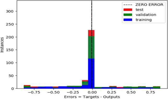
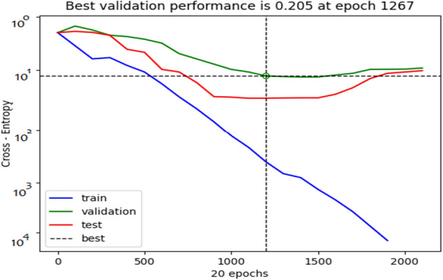
Furthermore, to support our case, the error histogram plot, cross entropy performance graph and the training, testing, validation and overall ROC curves for GTCC MFCC feature space and 1D DCGAN deep learning classifier are depicted in Figs. 31, 32, 33a–d respectively. The error histogram plot illustrates negligible data fitting error. Bearing it’s usual meaning, the cross entropy performance graph shows best validation performance of 0.205 at epoch 1267 for the GTCC+MFCC feature space with DCGAN classifier. For the ROC curves, the training and testing curves performs considerably better than validation as the curves are near the top left corner with AUC values 1. For more rigorous analysis, performance of the proposed 1D DCGAN network with the proposed GTCC+MFCC ensemble feature space is also evaluated on subject-independent scheme.
Fig. 31.
Error histogram plot for feature space with DCGAN classifier
Fig. 32.
Cross entropy performance plot for feature space with DCGAN classifier
Fig. 33.

ROC curves (one versus all classes) for feature space with DCGAN classifier
For subject-independent analysis
The extracted features from multiple subjects are intermixed and then passed through the 1D DCGAN model in proper dimensions with their optimised and satiating parameters and the performance metrics are discussed in this section. For subject-independent analysis, only the form in which the input features are fed to the network is changed. The rest of the entire operational strategy for the proposed 1D DCGAN classifier remains same. The training and the validation accuracies for the DCGAN classifier with the GTCC+MFCC features here is illustrated by the accuracy versus epoch curve (Fig. 34) for 1000 epochs. The curves converge really well. Table 9 gives the performance metrics for the proposed features with the proposed DCGAN model for subject-independent analysis. The accuracy for GTCC-MFCC feature space with the DCGAN model is 90.01% whereas for the GTCC+MFCC+CNN features is 89.81%. Hence their performances are comparable. Also, the loss versus epoch curve for the same model is shown in Fig. 35. Training and validation losses for the model are reported to be 1.1e-05 and 3.8e-03 respectively. The net Generator loss is 8.91e-03 and the net Discriminator loss is obtained as 2.4e-04. Figure 36 gives the mean absolute error for the DCGAN model with the GTCC+MFCC feature space whereas Fig. 37 gives the corresponding mean square error. It is observed that the mean absolute error metric values for training and validating the model with GTCC+MFCC feature space are 2.1e-09 & 1.2e-04. The mean squared error values for training and validating the same model are 4.4e-18 & 2.4e-08. It is thus inferred that the proposed 1D DCGAN model for subject-independent analysis of our proposed features yields comparatively inferior results to those obtained during subject-dependent analysis. Furthermore, to support our case, the error histogram plot, cross entropy performance graph and the training, testing, validation and overall ROC curves for GTCC MFCC feature space and 1D DCGAN deep learning classifier are depicted in Figs. 38, 39, 40a–d respectively. The error histogram plot illustrates very less data fitting error. Bearing it’s usual meaning, the cross entropy performance graph shows best validation performance of 0.220 at epoch 1270 for the GTCC+MFCC feature space with DCGAN classifier. For the ROC curves, the training & testing curves performs considerably better than validation as the curves are near the top left corner with AUC values 1. The results are less significant than those obtained in subject-dependent scheme and also with reduced accuracies.
Fig. 34.

Accuracy versus epoch curve for 1000 epochs for feature space and 1D DCGAN model for subject-independent scheme
Table 9.
Statistical measures for the proposed 1D DCGAN model with the proposed features for subject-independent analysis
| GTCC-MFCC-CNN | GTCC-MFCC | GTCC | ||||||||||||||||
|---|---|---|---|---|---|---|---|---|---|---|---|---|---|---|---|---|---|---|
| EOS | IOS | MOS | ROS | SROS | TOS | EOS | IOS | MOS | ROS | SROS | TOS | EOS | IOS | MOS | ROS | SROS | TOS | |
| Proposed 1D DCGAN | ACCURACY : 89.81% | ACCURACY : 90.01% | ACCURACY : 87.79% | |||||||||||||||
| Precision | 0.898 | 0.896 | 0.888 | 0.896 | 0.898 | 0.882 | 0.903 | 0.901 | 0.903 | 0.901 | 0.899 | 0.903 | 0.879 | 0.861 | 0.874 | 0.877 | 0.888 | 0.880 |
| Recall | 0.888 | 0.897 | 0.898 | 0.900 | 0.899 | 0.907 | 0.902 | 0.900 | 0.901 | 0.902 | 0.897 | 0.900 | 0.878 | 0.878 | 0.870 | 0.876 | 0.881 | 0.870 |
| F-Measure | 0.901 | 0.900 | 0.898 | 0.899 | 0.898 | 0.902 | 0.902 | 0.902 | 0.903 | 0.901 | 0.888 | 0.897 | 0.878 | 0.883 | 0.879 | 0.881 | 0.882 | 0.872 |
Bold values indicates the best accuracies obtained by our proposed techniques and are hence significant
Fig. 35.

Loss versus epoch curve for 1000 epochs for feature space and 1D DCGAN model for subject-independent scheme
Fig. 36.

Mean absolute error versus epoch curve for 1000 epochs for feature space and 1D DCGAN model for subject-independent scheme
Fig. 37.

Mean squared error versus epoch curve for 1000 epochs for feature space and 1D DCGAN model for subject-independent scheme
Fig. 38.

Error histogram plot for feature space with DCGAN classifier for subject-independent scheme
Fig. 39.

Cross entropy performance Plot for feature space with DCGAN classifier for subject-independent scheme
Fig. 40.

ROC curves (one versus all classes) for feature space with DCGAN classifier for subject-independent scheme
Statistical analysis
Certain statistical tests are carried out in this work to test the relevance of the extracted GTCC+MFCC+CNN features. Also, PNN and the proposed 1D DCGAN models are reliability tested through chi-squared goodness of fit test. Table 10 reports the statistical metric values for the tests when the samples in consideration are the extracted GTCC+MFCC+CNN features and the GTCC+MFCC ensemble feature space. A detailed discussion follows hereby:
Table 10.
Statistical measures for extracted CNN features with respect to GTCC+MFCC ensmeble feature space
| Tests | Values |
|---|---|
| T-test(t-statistic, p value) | (, 0.901) |
| KS-test(ks-statistic, p-value) | (1.03e-1, 0.14) |
| Energy distance | 8.19e-04 |
| Pearson’s r correlation coefficient | 0.916 |
T-test
A T-test is a prominent statistical test which is applied to carry out the comparison between the means of two groups. The main purpose of the test is in hypothesis testing to determine whether a process or treatment actually imposes effect on a population of interest, or whether the two processes or treatments are distinguished from one another. The null hypothesis for our case is that samples come from a population with same mean. Hence, it can be seen from Table 10, when GTCC+MFCC+CNN features are used in the 2-sample T-test with the ensemble feature space a t-value of -0.03 is obtained whereas a p-value of 0.901 is generated. Since the p-value is greater than 0.05 [significance level], it is inferred that the two samples come from the same population mean and the null hypothesis is not rejected. Also the samples have similar distribution which is visible from Fig. 41 as the test statistic follows a t-distribution under null hypothesis (p>0.05).
Fig. 41.

T-distribution curve for novel features
Kolmogorov–Smirnov test
Also known as the KS test, it is a non-parametric test of the equality of continuous or discontinuous, one-dimensional probability distributions that is used to compare a sample with reference probability distributions or to compare two samples. With a low KS-statistic value and a p-value of 0.14 (>0.05) as seen from Table 10, the hypothesis that multiple samples follow similar distributions cannot be declined. Hence, it is inevitably concluded that they come from homogeneous population means.
Energy distance test
This test gives the distance between probability distributions measured statistically. A value of 8.19e-04 as observed from Table 10, indicates that the GTCC+MFCC+CNN and GTCC+MFCC features follow indistinguishable distribution and are statistically similar.
Pearson’s r correlation coefficient
This test is basically employed to estimate the relation between two variables. Table 10 reports a value of 0.916 1. This shows that the two novel features in consideration i.e. GTCC+MFCC+CNN features and GTCC+MFCC feature space have analogous statistical properties.
Now, for the PNN and proposed 1D DCGAN classification models, chi-squared test is carried out with the proposed features (i.e. GTCC, GTCC+MFCC and CNN) separately (Table 11). The extracted CNN features in Table 11) refers to the GTCC+MFCC+CNN features.
Table 11.
Chi-squared test metric for PNN and DCGAN classification models with the proposed features: DOF - Degrees Of Freedom
| Samples | Statistic | p-value | DOF |
|---|---|---|---|
| PNN-CNN extracted features | 0.88 | 9.895e-1 | 6 |
| PNN-(GTCC+MFCC) | 0.89 | 9.894e-1 | 6 |
| PNN-GTCC | 0.98 | 9.863e-1 | 6 |
| DCGAN-CNN extracted features | 0.82 | 9.915e-1 | 6 |
| DCGAN-(GTCC+MFCC) | 0.81 | 9.918e-1 | 6 |
| DCGAN-GTCC | 0.91 | 9.887e-1 | 6 |
Chi-squared test
It is a test carried out to validate the performance of classification models. The threshold or significance level () is assumed to be 0.05 for our work. As per Table 11, all the p-statistic values are greater than the threshold. Hence, it is deduced that the classifier results are statistically significant as null hypothesis cannot be rejected. Also, it is proved that the results from the classifier with the proposed features hold good across all data sets and are repeatable. For statistical analysis of the state-of-the-art works mentioned in section "Comparative analysis with state-of-the-art methods", this test is carried out. According to Table 12, all the p-statistic values are more than the threshold and hence are statistically significant too. Also other statistical metrics i.e. precision, recall and f-measure for the state-of-the-art methods and the proposed models are already discussed in Tables 5, 6 and 8 respectively.
Table 12.
Chi-squared test metric for state-of-the-art works: DOF - Degrees Of Freedom
Comparative analysis with state-of-the-art methods
The previous works mostly dealt with binary classification problems whereas our work involves multi-class classification. A lot of traditional feature extraction methods have already been applied before. But we propose three novel feature extraction methods for ambulatory EEG data. The novel features thus extracted are GTCC, GTCC+MFCC ensemble feature space & the ones obtained automatically from the proposed 1D CNN model when the GTCC+MFCC feature space is fed into it. Also, we propose a 1D DCGAN model which performs considerably well for all the proposed features. Table 13 shows a comparison of our proposed methods with state of the art techniques on the basis of accuracy metric. It is clearly visible that our proposed techniques outperform all the other strategies. It is to be noted that all the state-of-the art methods used for comparative study are implemented on our dataset and then compared with our proposed techniques or models. Also a comparative analysis of the proposed network and a state-of-the-art technique is carried out on the basis of standard error metrics. Table 14 depicts the same. It can be seen from the table that the state-of-the art technique for basic CNN classifier along with DWT features yield maximum error values. With our proposed GTCC+MFCC ensemble feature space the standard error metric values reduce considerably. Finally our proposed model i.e. 1D DCGAN classifier along with GTCC+MFCC feature space generate the least error values, thus proving the superiority of our proposed technique in the context of our research.
Table 13.
Accuracies of the proposed methods with different state-of-art methodologies on the acquired dataset
| Reference | Classification models | Feature extraction techniques | Accuracy (%) | |
|---|---|---|---|---|
| Harshavarthini et al. (2019) | Machine learning based | PNN | DWT | 79.46 |
| Dutta et al. (2019) | PNN | MFCC | 89.5 | |
| Proposed Method I | PNN | GTCC | 91.14 | |
| Proposed Method II | PNN | GTCC+MFCC | 94.01 | |
| Proposed Method III | PNN | GTCC+MFCC+CNN | 94.89 | |
| Qayyum et al. (2018) | Deep learning based | CNN | DWT | 88.15 |
| Proposed Method IV | 1D DCGAN | GTCC | 92.69 | |
| Proposed Method V | 1D DCGAN | GTCC+MFCC+CNN | 96.14 | |
| Proposed Method VI | 1D DCGAN | GTCC+MFCC | 96.42 | |
Bold values indicates the accuracies obtained by our proposed methods
Table 14.
Standard error metrics for proposed and state-of-the-art models
| Models | TMAE | TMSE | VMAE | VMSE |
|---|---|---|---|---|
| CNN-DWT (Qayyum et al. 2018) | 1.1e-07 | 1.2e-14 | 1.9e-03 | 3.6e-06 |
| CNN-(GTCC+MFCC) | 1.2e-10 | 1.4e-20 | 2.3e-06 | 5.3e-12 |
| Proposed 1D DCGAN-(GTCC+MFCC) | 2.7e-11 | 7.29e-22 | 3.1e-07 | 9.6e-14 |
Bold value indicates the minimum error obtained from our proposed technique
TMAE Training Mean Absolute Error, TMSE Training Mean Square Error, VMAE Validation Mean Absolute Error, VMSE Validation Mean Square Error
Conclusion and future work
Novel features are introduced through the feature extraction strategies for human cognitive state classification in this paper. The states considered are EOS, MOS, ROS, TOS, SROS and IOS respectively. EEG signals are acquired by creation of a novel event driven environment for cognitive state simulation. The experiments are conducted on acquired dataset. Proposed GTCC feature extraction technique gives better performance than the other features as analysed from the results obtained. The patent characteristics of GTCC feature extraction technique accounts for its superior performance with respect to MFCC or the conventional DWT technique when applied on the ambulatory EEG dataset in this work. After a rigorous analysis on importance of features through FDR and logistic regression strategies, GTCC features are found to be most discriminating. Table 5, shows that all the classifiers used in our work demonstrate better accuracies for GTCC features. Although all the classifiers exhibit better performances for GTCC features, an overall accuracy of 91.14% is obtained for PNN utilizing GTCC. It is ascertained to be the best one. After the individual features are ascertained, ensemble feature spaces are explored and proposed in this work. Of all the ensemble feature spaces (GTCC+MFCC. GTCC+DWT & MFCC+DWT) proposed in this work, GTCC+MFCC performed the best. The superior discriminative ability of the proposed GTCC+MFCC feature space is exhibited by the FDR and the LR scores. Also, a 1D CNN model is proposed in this work, which is used initially for automatic extraction of novel features. These features are obtained by passing GTCC+MFCC ensemble feature space into the CNN model. The extracted GTCC+MFCC+CNN features are equally important as that of the GTCC MFCC feature space as per the FDR and the LR scores. The GTCC+MFCC+CNN features are passed through the machine learning classifiers and tested. Also, Table 6 depicts that all the proposed ensemble feature spaces achieve superior accuracies when compared to the individual features . This is because of the increase in the diversity amongst the features when the feature sets are combined. According to the same table it is inferred that, the GTCC +MFCC +CNN features exhibit best performance with the PNN classifier with an accuracy of 94.89% followed by GTCC-MFCC or GTCC+MFCC feature space. The GTCC MFCC feature space showcases an accuracy of 94.01% with the PNN classifier. Hence it is deduced that the GTCC+MFCC and the GTCC+MFCC+CNN features exhibit comparable performances with an accuracy difference of ±0.88. Finally, a 1D DCGAN deep learning model is proposed in this work. All the proposed features are passed through this model and they perform exceptionally well as can be seen in Table 8. Also, in Table 8, a short analysis is carried out between our proposed 1D DCGAN model being used as a classifier and a basic CNN model. It is seen that our model outperforms the basic CNN model with all the proposed features. Also, section "Comparative analysis with state-of-the-art methods" is a support to our claim that our proposed model along with the proposed features is not only superior in performance but more effective than the state-of-the-art methods. Thus, in this paper a new and better feature representation prototype is proposed for cognitive state recognition. These decision support systems require very less human interference and are highly contributing in the field of healthcare pertaining to reduction of stress, suicidal possibilities, etc. This work thus motivates the creation of cost-effective estimators which would unveil human cognitive behaviors for various environmental circumstance based on ambulatory EEG signal analysis. Most of the nations, especially resource poor ones, have a shortage of awareness guides, healthcare executives, infrastructure, etc. Thus, there is always a burden of both resources as well as financial constraints due to inadequate health literacy and similar other reasons. Furthermore, treatment centres for patients especially hospitals lack proper infrastructure and skilled personnel which makes access to the services of healthcare domain much more expensive. Thus, in our proposed system for cognitive behavior identification of human beings, the ambulatory EEG data collection is done in lab environment using power point slides, videos and hence are highly affordable. With the automation in the diagnosis of our proposed system, the mental states can be predicted at an early stage. This would essentially cause the healthcare people to focus on more complex cases rather than monitoring activities. Also, with this system for any kind of medical diagnosis, the number of patient tests and hospital stay durations will be considerably reduced to a great extent. All these factors cumulatively will cater to the cost reduction and hence our proposed system is cost-effective.
Future work involves exploring other classification strategies and development of a cognitive tool which might help the resourc0e poor countries in the healthcare domain.
Acknowledgements
We are extremely thankful to Science and Engineering Research Board (SERB), DST, Govt. of India to support this research work. The Kinect v2.0 sensors and the EEG headset used in our research experiment are purchased from the project funded by SERB with FILE NO: ECR/2017/000408. We would also like to extend our sincere thanks to the students of Department of Computer Science and Engineering, NIT Rourkela for their uninterrupted cooperation and participation catering to the data collection.
Funding
This study was funded by SERB, DST (Department of Science and Technology, Govt. Of India) for the Project file no. ECR/2017/000408.
Data Availability
The datasets generated during and/or analysed during the current study are available from the corresponding author on reasonable request.
Declarations
Conflict of interest
The authors declare that they have no conflict of interest.
Informed consent
Informed consent was obtained from all individual participants (human subjects) included in the study.
Footnotes
Publisher's Note
Springer Nature remains neutral with regard to jurisdictional claims in published maps and institutional affiliations.
References
- Abdulla WH (2002) Auditory based feature vectors for speech recognition systems. Adv Commun Softw Technol pp 231–236
- Agarwal R, Gotman J. Computer-assisted sleep staging. IEEE Trans Biomed Eng. 2001;48(12):1412–1423. doi: 10.1109/10.966600. [DOI] [PubMed] [Google Scholar]
- Albayrak M. The detection of an epileptiform activity on eeg signals by using data mining process. Technol Appl Sci. 2009;4(1):1–12. [Google Scholar]
- Amores J, Benavides X, Maes P (2016) Psychicvr: Increasing mindfulness by using virtual reality and brain computer interfaces. In: Proceedings of the 2016 CHI conference extended abstracts on human factors in computing systems, pp 2–2
- Bajaj V, Pachori RB. Automatic classification of sleep stages based on the time-frequency image of eeg signals. Comput Methods Programs Biomed. 2013;112(3):320–328. doi: 10.1016/j.cmpb.2013.07.006. [DOI] [PubMed] [Google Scholar]
- Bao FS, Lie DYC, Zhang Y (2008) A new approach to automated epileptic diagnosis using eeg and probabilistic neural network. In: 2008 20th IEEE international conference on tools with artificial intelligence, IEEE, vol 2, pp 482–486
- Bashivan P, Rish I, Heisig S (2016) Mental state recognition via wearable eeg. arXiv preprint arXiv:160200985
- Bruzzo AA, Gesierich B, Santi M, Tassinari CA, Birbaumer N, Rubboli G. Permutation entropy to detect vigilance changes and preictal states from scalp eeg in epileptic patients a preliminary study. Neurol Sci. 2008;29(1):3–9. doi: 10.1007/s10072-008-0851-3. [DOI] [PubMed] [Google Scholar]
- Castellanos NP, Makarov VA. Recovering eeg brain signals: artifact suppression with wavelet enhanced independent component analysis. J Neurosci Methods. 2006;158(2):300–312. doi: 10.1016/j.jneumeth.2006.05.033. [DOI] [PubMed] [Google Scholar]
- Cheng O, Abdulla W, Salcic Z (2005) Performance evaluation of front-end algorithms for robust speech recognition. In: Proceedings of the eighth international symposium on signal processing and its applications, 2005, IEEE, vol 2, pp 711–714
- Cowling M, Sitte R. Comparison of techniques for environmental sound recognition. Pattern Recogn Lett. 2003;24(15):2895–2907. doi: 10.1016/S0167-8655(03)00147-8. [DOI] [Google Scholar]
- D’Alessandro M, Vachtsevanos G, Hinson A, Esteller R, Echauz J, Litt B (2001) A genetic approach to selecting the optimal feature for epileptic seizure prediction. In: 2001 Conference proceedings of the 23rd annual international conference of the ieee engineering in medicine and biology society, IEEE, vol 2, pp 1703–1706
- Daubechies I. The wavelet transform, time-frequency localization and signal analysis. IEEE Trans Inf Theory. 1990;36(5):961–1005. doi: 10.1109/18.57199. [DOI] [Google Scholar]
- Dimoulas C, Kalliris G, Papanikolaou G, Kalampakas A. Long-term signal detection, segmentation and summarization using wavelets and fractal dimension: a bioacoustics application in gastrointestinal-motility monitoring. Comput Biol Med. 2007;37(4):438–462. doi: 10.1016/j.compbiomed.2006.08.013. [DOI] [PubMed] [Google Scholar]
- Dutta S, Hazra S, Nandy A (2019) Human cognitive state classification through ambulatory eeg signal analysis. In: International conference on artificial intelligence and soft computing, pp 169–181, Springer, Berlin
- Eronen AJ, Peltonen VT, Tuomi JT, Klapuri AP, Fagerlund S, Sorsa T, Lorho G, Huopaniemi J. Audio-based context recognition. IEEE Trans Audio Speech Lang Process. 2005;14(1):321–329. doi: 10.1109/TSA.2005.854103. [DOI] [Google Scholar]
- Fraiwan L, Lweesy K, Khasawneh N, Wenz H, Dickhaus H. Automated sleep stage identification system based on time-frequency analysis of a single eeg channel and random forest classifier. Comput Methods Programs Biomed. 2012;108(1):10–19. doi: 10.1016/j.cmpb.2011.11.005. [DOI] [PubMed] [Google Scholar]
- Gajbhiye P, Mingchinda N, Chen W, Mukhopadhyay SC, Wilaiprasitporn T, Tripathy RK. Wavelet domain optimized savitzky-golay filter for the removal of motion artifacts from eeg recordings. IEEE Trans Instrum Meas. 2020;70:1–11. doi: 10.1109/TIM.2020.3041099. [DOI] [Google Scholar]
- Geng S, Zhou W, Yuan Q, Cai D, Zeng Y. Eeg non-linear feature extraction using correlation dimension and hurst exponent. Neurol Res. 2011;33(9):908–912. doi: 10.1179/1743132811Y.0000000041. [DOI] [PubMed] [Google Scholar]
- Glavinovitch A, Swamy M, Plotkin E (2005) Wavelet-based segmentation techniques in the detection of microarousals in the sleep eeg. In: 48th Midwest symposium on circuits and systems, 2005, IEEE, pp 1302–1305
- Harshavarthini S, Aswathy M, Harshini P, Priyanka G. Automated epileptic seizures detection and classification. Int J Sci Res Comput Sci Eng Inf Technol. 2019;5(1):555–560. [Google Scholar]
- Jahankhani P, Kodogiannis V, Revett K (2006) Eeg signal classification using wavelet feature extraction and neural networks. In: IEEE John Vincent Atanasoff 2006 international symposium on modern computing (JVA’06), IEEE, pp 120–124
- Kandel ER, Schwartz JH, Jessell TM, of Biochemistry D, Jessell MBT, Siegelbaum S, Hudspeth A (2000) Principles of neural science, vol 4. McGraw-hill New York
- Kannathal N, Choo ML, Acharya UR, Sadasivan P. Entropies for detection of epilepsy in eeg. Comput Methods Programs Biomed. 2005;80(3):187–194. doi: 10.1016/j.cmpb.2005.06.012. [DOI] [PubMed] [Google Scholar]
- Krizhevsky A, Sutskever I, Hinton GE. Imagenet classification with deep convolutional neural networks. Commun ACM. 2017;60(6):84–90. doi: 10.1145/3065386. [DOI] [Google Scholar]
- Lajnef T, Chaibi S, Ruby P, Aguera PE, Eichenlaub JB, Samet M, Kachouri A, Jerbi K. Learning machines and sleeping brains: automatic sleep stage classification using decision-tree multi-class support vector machines. J Neurosci Methods. 2015;250:94–105. doi: 10.1016/j.jneumeth.2015.01.022. [DOI] [PubMed] [Google Scholar]
- Lakhan P, Banluesombatkul N, Changniam V, Dhithijaiyratn R, Leelaarporn P, Boonchieng E, Hompoonsup S, Wilaiprasitporn T. Consumer grade brain sensing for emotion recognition. IEEE Sens J. 2019;19(21):9896–9907. doi: 10.1109/JSEN.2019.2928781. [DOI] [Google Scholar]
- LeCun Y, Bengio Y, Hinton G. Deep learning. Nature. 2015;521(7553):436–444. doi: 10.1038/nature14539. [DOI] [PubMed] [Google Scholar]
- Mohseni HR, Maghsoudi A, Shamsollahi MB (2006) Seizure detection in eeg signals: a comparison of different approaches. In: 2006 International conference of the IEEE engineering in medicine and biology society, IEEE, pp 6724–6727 [DOI] [PubMed]
- Newland DE (2012) An introduction to random vibrations, spectral and wavelet analysis. Courier Corporation
- Nixon M, Aguado A. Feature extraction and image processing for computer vision. Cambridge: Academic press; 2019. [Google Scholar]
- Oropesa E, Cycon HL, Jobert M (1999) Sleep stage classification using wavelet transform and neural network. International computer science institute
- Pan ST, Kuo CE, Zeng JH, Liang SF. A transition-constrained discrete hidden markov model for automatic sleep staging. Biomed Eng Online. 2012;11(1):52. doi: 10.1186/1475-925X-11-52. [DOI] [PMC free article] [PubMed] [Google Scholar]
- Petrosian A, Prokhorov D, Homan R, Dasheiff R, Wunsch D., II Recurrent neural network based prediction of epileptic seizures in intra-and extracranial eeg. Neurocomputing. 2000;30(1–4):201–218. doi: 10.1016/S0925-2312(99)00126-5. [DOI] [Google Scholar]
- Plis SM, Hjelm DR, Salakhutdinov R, Allen EA, Bockholt HJ, Long JD, Johnson HJ, Paulsen JS, Turner JA, Calhoun VD. Deep learning for neuroimaging: a validation study. Front Neurosci. 2014;8:229. doi: 10.3389/fnins.2014.00229. [DOI] [PMC free article] [PubMed] [Google Scholar]
- Pradhan N, Sadasivan P, Arunodaya G. Detection of seizure activity in eeg by an artificial neural network: A preliminary study. Comput Biomed Res. 1996;29(4):303–313. doi: 10.1006/cbmr.1996.0022. [DOI] [PubMed] [Google Scholar]
- Procházka A, Jech J, Smith J (1994) Wavelet transform use in signal processing. In: 31st International conference in acoustics, pp 209–213
- Qayyum A, Khan MA, Mazher M, Suresh M (2018) Classification of eeg learning and resting states using 1d-convolutional neural network for cognitive load assesment. In: 2018 IEEE student conference on research and development (SCOReD), IEEE, pp 1–5
- Rabaoui A, Lachiri Z, Ellouze N (2007) Towards an optimal feature set for robustness improvement of sounds classification in a hmm-based classifier adapted to real world background noise. In: Proceedings of the 4th International Multi-Conference on Systems, Signals and Devices
- Radha M, Garcia-Molina G, Poel M, Tononi G (2014) Comparison of feature and classifier algorithms for online automatic sleep staging based on a single eeg signal. In: 2014 36th Annual International Conference of the IEEE Engineering in Medicine and Biology Society, IEEE, pp 1876–1880 [DOI] [PubMed]
- Sanei S, Chambers JA. EEG signal processing. New Jersey: John Wiley and Sons; 2013. [Google Scholar]
- Sawangjai P, Hompoonsup S, Leelaarporn P, Kongwudhikunakorn S, Wilaiprasitporn T. Consumer grade eeg measuring sensors as research tools: a review. IEEE Sens J. 2019;20(8):3996–4024. doi: 10.1109/JSEN.2019.2962874. [DOI] [Google Scholar]
- Schluter R, Bezrukov I, Wagner H, Ney H (2007) Gammatone features and feature combination for large vocabulary speech recognition. In: 2007 IEEE International Conference on Acoustics, Speech and Signal Processing-ICASSP’07, IEEE, vol 4, pp IV–649
- Selesnick IW, Baraniuk RG, Kingsbury NC. The dual-tree complex wavelet transform. IEEE Signal Process Mag. 2005;22(6):123–151. doi: 10.1109/MSP.2005.1550194. [DOI] [Google Scholar]
- Şen B, Peker M. Novel approaches for automated epileptic diagnosis using fcbf selection and classification algorithms. Turk J Electr Eng Comput Sci. 2013;21(Sup 1):2092–2109. doi: 10.3906/elk-1203-9. [DOI] [Google Scholar]
- Şen B, Peker M, Çavuşoğlu A, Çelebi FV. A comparative study on classification of sleep stage based on eeg signals using feature selection and classification algorithms. J Med Syst. 2014;38(3):18. doi: 10.1007/s10916-014-0018-0. [DOI] [PubMed] [Google Scholar]
- Shao Y, Wang D, (2008) Robust speaker identification using auditory features and computational auditory scene analysis. In: IEEE International conference on acoustics, speech and signal processing, IEEE, pp 1589–1592
- Shao Y, Jin Z, Wang D, Srinivasan S, (2009) An auditory-based feature for robust speech recognition. In: IEEE international conference on acoustics, speech and signal processing, IEEE, pp 4625–4628
- Sjöberg J, Ljung L. Overtraining, regularization and searching for a minimum, with application to neural networks. Int J Control. 1995;62(6):1391–1407. doi: 10.1080/00207179508921605. [DOI] [Google Scholar]
- Thakor NV, Sherman DL. Neural Engineering. Berlin: Springer; 2013. Eeg signal processing: Theory and applications; pp. 259–303. [Google Scholar]
- Valero X, Alias F. Gammatone cepstral coefficients: biologically inspired features for non-speech audio classification. IEEE Trans Multimed. 2012;14(6):1684–1689. doi: 10.1109/TMM.2012.2199972. [DOI] [Google Scholar]
- Weng W, Khorasani K. An adaptive structure neural networks with application to eeg automatic seizure detection. Neural Networks. 1996;9(7):1223–1240. doi: 10.1016/0893-6080(96)00032-9. [DOI] [PubMed] [Google Scholar]
- Wolpaw JR, Birbaumer N, McFarland DJ, Pfurtscheller G, Vaughan TM. Brain-computer interfaces for communication and control. Clin Neurophysiol. 2002;113(6):767–791. doi: 10.1016/S1388-2457(02)00057-3. [DOI] [PubMed] [Google Scholar]
- Yuen CT, San San W, Seong TC, Rizon M (2009) Classification of human emotions from eeg signals using statistical features and neural network. Int J Integ Eng 1(3)
Associated Data
This section collects any data citations, data availability statements, or supplementary materials included in this article.
Data Availability Statement
The datasets generated during and/or analysed during the current study are available from the corresponding author on reasonable request.