ProtCHOIR: a tool for proteome-scale generation of homo-oligomers

Abstract

The rapid developments in gene sequencing technologies achieved in the recent decades, along with the expansion of knowledge on the three-dimensional structures of proteins, have enabled the construction of proteome-scale databases of protein models such as the Genome3D and ModBase. Nevertheless, although gene products are usually expressed as individual polypeptide chains, most biological processes are associated with either transient or stable oligomerisation. In the PDB databank, for example, ~40% of the deposited structures contain at least one homo-oligomeric interface. Unfortunately, databases of protein models are generally devoid of multimeric structures. To tackle this particular issue, we have developed ProtCHOIR, a tool that is able to generate homo-oligomeric structures in an automated fashion, providing detailed information for the input protein and output complex. ProtCHOIR requires input of either a sequence or a protomeric structure that is queried against a pre-constructed local database of homo-oligomeric structures, then extensively analyzed using well-established tools such as PSI-Blast, MAFFT, PISA and Molprobity. Finally, MODELLER is employed to achieve the construction of the homo-oligomers. The output complex is thoroughly analyzed taking into account its stereochemical quality, interfacial stabilities, hydrophobicity and conservation profile. All these data are then summarized in a user-friendly HTML report that can be saved or printed as a PDF file. The software is easily parallelizable and also outputs a comma-separated file with summary statistics that can straightforwardly be concatenated as a spreadsheet-like document for large-scale data analyses. As a proof-of-concept, we built oligomeric models for the Mabellini Mycobacterium abscessus structural proteome database. ProtCHOIR can be run as a web-service and the code can be obtained free-of-charge at http://lmdm.biof.ufrj.br/protchoir.

Introduction

Despite decades of development in protein structure determination methods, even after the increased throughput induced by the implementation of the structural genomics initiatives, the number of solved protein structures still lags far behind that of sequenced genes [1–3]. On the other hand, emerging computational techniques, including big data analysis and machine learning methods, are increasingly data-hungry and rely upon the availability of a large amount of data to perform optimally [4].

In this sense, protein modelling methods are extremely useful, enabling the generation of a much larger body of (albeit predicted) structural data, as long as a given accuracy trade-off is admitted, and the resulting models are carefully assessed [5]. To date, comparative modelling remains the most reliable method of protein structure prediction [6, 7], as it extracts spatial information of known structures and transposes it into a new, likely homologous, context.

Among other applications, protein models can be of use in binding-site identification, ligand prospection and rationalizing known experimental observations [8]. Large-scale assessment of druggability is also a powerful tool for the prospection of new targets, especially for new antimicrobial agents, as it is particularly difficult to pinpoint novel bacterial targets that are simultaneously essential, bio-accessible, specific and druggable [9, 10]. Given these goals, several organism-focused and general-purpose protein model databases have been established, e.g. Modbase [11], Genome3D [12, 13], Chopin [14], Mabellini [15] and SARS-CoV-2 3D [16].

Analysing protomeric structures is certainly an important endeavour but does not constitute the complete scenario. Analyses of higher order homo- and hetero-oligomeric structures are essential for understanding the complex multicomponent regulatory systems, which provide alternative targets for therapeutic intervention [17–19]. Nevertheless, our knowledge of the atomistic details of protein complexes is much more limited than the number of protein interactions currently known to take place. In fact, it is estimated that cocrystals and modelled complexes represent as little as 6% of all known interactions [20].

Automating the comparative modelling even of homo-oligomeric complexes is a highly demanding task. Homologues can have different oligomeric assemblies, and thus, the use of a homologue with an experimentally defined oligomeric structure to model an oligomeric structure has to be treated with caution. Furthermore, even the determination of the quaternary structure in protein crystals could be ambiguous, and it is estimated that ~15% of the quaternary structures in the PDB are wrongly annotated mostly due to the cumbersome task of distinguishing biologically relevant contacts from crystallization-induced ones [21, 22]. Of course, the usual problems with modelling monomers/protomers using structures of homologues still occur. These include low-resolution structures, missing amino acids or individual sidechains due to disorder in the template, insertions and deletions of the protein sequence to be modelled relative to the preferred template structures deposited in the PDB, etc.

Regarding modelling hetero-oligomers, an extra layer of uncertainty comes into play, as the sequences of the proteins that form these complexes must either be provided concurrently or, given protomeric structures, the method should allow identification of correct interacting partners.

Here, we focus on building a high-throughput and information-rich pipeline, as a novel tool to cope with the need of building proteome-scale comparative models of homo-oligomeric structures. Additionally, we tested the performance of the pipeline using Mycobacterium abscessus as a model organism, ultimately generating structures for nearly 2000 different homo-oligomeric protein complexes.

Methods

Local homo-oligomers database creation (CHOIRDB)

After installation of the required software and the ProtCHOIR pipeline, the first step is the creation of a local set of structure and sequence databases collectively referred to as CHOIRDB (Figure 1). This initial set-up can be accomplished in a relatively simple way, by using the update flag (−u) in the command-line.

Figure 1 .

Schematic representation of the structuring of the ProtCHOIR database. Local mirrors for PDB and PDB1 (assemblies) repositories are created, before assessing the existence of homo-oligomeric interfaces to create the homo-oligomers archive. Sequences of monomers, homo-oligomers and hetero-oligomers are recorded individually and used to create BLAST databases. Once a PDB entry is assessed, the database records a timestamp to avoid reassessment of the same entry in subsequent updates, unless that entry is updated in the original wwPDB repository; all this information is recorded in the Stats folder.

This custom database contains a copy of the PDB (/choirdb/pdb) and PDB1 (/choirdb/pdb1) repositories and from these, ProtCHOIR selects the structures that contain at least one homo-oligomeric interface to create a new structural database containing homo-oligomers (/choirdb/pdb_homo_archive). To accomplish this classification, we employed Parasail [23] (to perform sequence alignments) and Biopython [24] (in order to check interfacial contacts).

Briefly, the PDB (asymmetric units) and PDB1 (homo-oligomers) repositories are initially mirrored using the Rsync application. After the mirrored directories have been updated, the oligomer database curation begins. Curation involves:

• (i) Assessment of the bioassembly file size: files with size above 10 Mb are discarded, for they are usually large viral capsids, and the interface analysis time can become prohibitive.

• (ii) Parsing of the bioassemblies using Biopython and chain counting: assemblies with chain count between 1 and 60 are kept for further analysis;

• (iii) Extraction of chain sequences and pairwise semi-global sequence analysis: each chain in the analyzed entry is compared with all other chains in the same entry, in order to determine whether the entry contains a homo-oligomer. This alignment is accomplished using the Parasail [23] software, with the semi-global alignment algorithm. Entries in which all sequences are nearly identical (identity >90%) are stored in the database, while those containing at least two (but not all) near-identical sequences are further analyzed to check for homo-oligomeric interfaces.

• (iv) Homo-oligomeric interface detection: Biopython [25] is used to perform a pairwise neighbour search between the atoms of chains with near-identical sequences. If at least one contact (i.e. an interatomic distance under 3.5 Å) between two near-identical chains is found, the entry is stored in the database.

Furthermore, the sequences of the monomers, homo-oligomers and hetero-oligomers are also stored as individual BLAST [26] databases. The retrieved PDB entries are recorded to prevent re-assessment in future database updates unless the entry has been updated in the PDB repository itself. The processing of entries is conditioned upon timestamp-checking of each entry file.

The sequences of all structures are collected into three distinct sets: (i) homo-oligomeric sequences (HomoDB), (ii) hetero-oligomeric sequences (HeteroDB) and (iii) monomeric sequences (MonoDB). Blast databases are created for each one of the specified sets. Furthermore, a BLAST database is also generated for the UniProt Reference Clusters (Uniref50) [27] sequence database, which will allow for the alignment of homologues and entropy calculation. The fully detailed procedure for the generation of the full CHOIRDB can be found in Figure S1, see Supplementary Data available online at http://bib.oxfordjournals.org/.

The local databases can be easily updated by running the ProtCHOIR software with the -u flag, in which case the PDB and PDB1 repositories will be mirrored and only newly added proteins will be assessed by the curation process.

Section 1: protomer analysis

The ProtCHOIR protocol for the generation of homo-oligomers can be conceptually split into three main sections: (i) analysis of the input protomer structure, (ii) homo-oligomer generation and (iii) final homo-oligomer analysis (Figure 2). After the models are built and evaluated, a final HTML report is generated containing relevant information about the system being modelled. The first section, i.e. the analysis of the protomer, is designed to accept either a PDB structure or a protein sequence in the FASTA format as input.

Figure 2 .

ProtCHOIR pipeline. ProtCHOIR has been organized in three main sections: (i) analysis of the input protomer (green section), (ii) construction of the homo-oligomeric model (light red section) and (iii) analysis of the final model (blue section). All sections use common functions available in the ProtCHOIR toolbox. The most time-consuming steps (darker-coloured boxes) were identified and the Multiprocess python package was employed to expedite them. Red arrows indicate steps performed only when run in default mode; i.e. when an initial structure for the protomer is given as input. Blue arrows indicate the information flow when building monomeric/protomeric structures. Dashed arrows indicate data that are collected into the final report.

Subsection 1 [a] and 1 [b]: load input and oligomeric homologues search

The first step involves the parsing of the input file and retrieval of the sequence from the structure, which is accomplished using Biopython. The protomer sequence is then queried, using PSI-BLAST [28], against the local database in order to identify possible homo-oligomeric templates. The sequence is also queried against local monomer and hetero-oligomer sequence databases to assess the likelihood of it being an actual homo-oligomer.

This likelihood is expressed in terms of a fractional score (Eq. 1), consisting of the ratio between the maximum PSI-BLAST score obtained for the Homo-DB and the maximum score obtained for the MonoDB or HeteroDB. This score is termed H3O score (Homo Oligomeric Over Other) and it prevents the construction of complexes that are obviously not homo-oligomeric through a tolerance parameter that can be tweaked by the user (defaults to 0.15 tolerance; i.e. the PSI-BLAST score for the HomoDB can be up to 15% lower than the score for the MonoDB or HeteroDB, and the building of a homo-oligomer will still be attempted).

(1)

If the user explicitly requests the construction of monomers through the option—allow-monomers, homo-oligomers will only be built if the best PSI-BLAST hits are homo-oligomeric, thus ignoring the tolerance threshold. Otherwise, the tolerance threshold is enforced and homo-oligomers are built as described above.

Subsection 1 [c]

After ensuring that there are suitable templates in the local HomoDB, ProtCHOIR runs the PISA software on the input protomer structure (when available) to assess the total solvent-accessible surface area (SASA) and relative SASA per residue, which will integrate a final HTML report. Relative residue SASA is bar-plotted in terms of the percent exposed areas, relative to the theoretical total SASA [29], and colour-coded according to Wimley–White hydrophobicity-scale [30]. The SASA of conserved and hydrophobic residues in the protomer will be compared with that of model homo-oligomers, in order to assess their overall accuracy (c.f. Subsection 3 [I]).

The TMHMM [31] program is also run on the input sequence to detect plausible transmembrane helices, which will influence the interface-scoring protocol executed later in the pipeline. Additionally, MolProbity [32] is run on the input protomer structure (when available) to assess the global structural quality of the input protomer.

Subsection 1 [d]

The program then performs a new PSI-BLAST search, this time against the UniRef50 database, to retrieve up to 100 homologous sequences that are subsequently aligned using MAFFT [33] and used to assess the sequence relative informational entropy [34] using Eq. 2

(2)

where represents the observed frequency of residue type in the aligned column, is the number of residue types in the columns and is the background frequency of residue type . is the relative entropy or Kullback–Liebler divergence ) between the background distribution of amino acids and the actual distribution of residues in each position of the multiple sequence alignment.

The relative entropies then undergo a Z-score normalization and each position in the sequence is assigned a Z-Entropy (Eq. 3).

(3)

where is the normalized entropy, is the mean relative entropy and is the standard deviation of the relative entropy scores. These values are used to evaluate the final quality of the modelled oligomers and also to better characterize the biological context of the concerned protein; in this sense, the values are plotted onto a bar-chart that composes the final HTML report and then projected onto the cartoon structure of the input protomer.

Subsection 1 [e]: oligomeric homologues analysis

The candidate hits found through the first PSI-BLAST run are evaluated to check whether the relevant chains are in close contact, i.e. if the relevant chains form homo-oligomeric interfaces. This step is again accomplished using Biopython and the interfaces are recorded in a dictionary-type object and plotted graphically using Matplotlib [35] and NetworkX [36].

Section 2: oligomer assembly

Subsection 2 [a]: structural template selection

After the detection of the most suitable hits and relevant chains in each oligomer, ProtCHOIR proceeds to the modelling of oligomeric complexes. If ProtCHOIR is run in the default (structure) mode, GESAMT [37] is used to superimpose the input protomer onto each relevant chain of the PSI-BLAST-retrieved hits and evaluate which hit provides the best average structural agreement (in terms of Q-Scores). If the software is run in sequence mode, then the best hit found by PSI-Blast is straightforwardly used instead.

Subsection 2 [b]: alignment generation

In the default mode, sequence alignment is derived directly from per-chain GESAMT-generated structural alignments, which is achieved by individually superimposing the input protomer to each relevant chain. In sequence mode, Modeller [38] is used to align the protomer sequence to each one of the relevant chains.

The alignments are then split into 30-residue windows and scored relative to the highest possible score (i.e. a theoretical alignment to a sequence identical to the input). The score assigned to each 30-residue window is based on the BLOSUM62 [39] matrix, modified to contain no negative values. This procedure is performed to guarantee that no stretch (of 30 residues by default) of the modelled protein will have unacceptable structural quality; this is especially useful in sequence-mode and the thresholds can be adjusted via command-line options.

Subsection 2 [c]: homo-oligomer modelling

The oligomeric models are then generated using Modeller, and options such as the number of output models, the level of refinement and whether or not to apply symmetry constraints can be controlled by the user through the use of command-line flags (−m, −r and −symmetry, respectively). If more than one model is requested, both their construction and subsequent analysis are performed using multiple processing cores.

Section 3: oligomer analysis

The generated models are subjected to a structure analysis involving three steps: (i) calculation of the RMSD to the used template, (ii) interface analysis and (iii) MolProbity analysis.

The RMSD calculation is a straightforward procedure and is performed using GESAMT, which is able to calculate the RMSD for the whole complex (not only one chain) in reasonable time.

The interface analysis takes two major aspects into consideration: the pre- versus post-oligomerization SASA and the PISA-calculated interface parameters. The SASA of the residues in the post-oligomerization protomer structure is measured for (i) conserved residues, (ii) hydrophobic residues and (iii) total SASA. From the comparison with the pre-oligomerization protomer values, ProtCHOIR determines the total SASA reduction (), the hydrophobic SASA reduction () and the conserved residues SASA reduction () and uses these values to calculate the Hydrophobic Surface Score (; Eq.4), the Conserved Surface Score (; Eq. 5) and finally the Surface Score (; Eq. 6).

(4)

(5)

(6)

Thus, this method would maximally score (i.e. ) the oligomeric model if the reduction of the relative conserved and hydrophobic SASA are both at least three times higher than the overall SASA reduction.

The PISA-calculated interface parameters of the template structure are then compared with those of the modelled oligomer. In total, five different parameters are assessed: interface area, interfacial free energy of dissociation, hydrogen bond count, salt bridge count and disulfide bond count. All these are taken into consideration, with different weights, to calculate the Interface Score (; Eq. 7) and are individually plotted and added to the final HTML report.

(7)

All parameters in the equation above are relative to those of the template structure. Relative hydrogen bond count () and relative energy () parameters have double weight, the relative salt bridge count () has triple weight and the relative disulfide bridges count () has four times the weight of the area parameter (). If any of the values is non-existent for both template and model, they are removed from the weighted averaging.

Finally, MolProbity clashscore is used to assess the stereochemical quality of the modelled oligomer, and the final value is compared with that of the template and used to calculate the Quality Score (; Eq. 8). Additionally, all template’s and model’s MolProbity-calculated output parameters are plotted onto a radar plot that is also presented in the final HTML report and allows for easy visual comparison between the stereochemical quality of the model and the template.

(8)

Where is the difference between the model’s template’s Molprobity Clashscore. The final ProtCHOIR score is given as the arithmetic average of the three individual scores, unless when run in sequence mode, in which case the Surface Score is not available, or when generating monomers/protomers in which case both Surface and Interface scores are unavailable.

Benchmarking dataset and accuracy assessment

To evaluate the accuracy of the developed pipeline, we set up a diverse benchmarking dataset consisting of 141 proteins with oligomeric states ranging from dimer to octamer, having proteins in the following SCOP [40] classes: Mainly Alpha, Mainly Beta and Alpha Beta (Table S1, see Supplementary Data available online at http://bib.oxfordjournals.org/) gathered from the PDB database in as bioassemblies. Using this dataset, we executed ProtCHOIR with and without the ‘–sequence-mode’ flag and measured the accuracies according to two different criteria: the correctness of the expected number of chains (Figure 3) and the RMSD between template and model (Figure 4).

Figure 3 .

Comparison of the percent oligomerization state accuracy (i.e. correct number of chains) in sequence and structure modes for proteins in each of the three main SCOP structural classes: Alpha Beta (A), Mainly Alpha (B), Mainly Beta (C) and the entire dataset (D). The percent oligomerization state accuracy has been calculated independently for complexes ranging from 2 to 8 chains.

Figure 4 .

RMSD of the models against their templates separated by correct and incorrect oligomerization states and sequence and structure mode. The numbers above the boxes show how many elements are present in that particular category.

Furthermore, to compare our method with a widely accepted software, we selected a representative protein from each class (maily alpha, mainly beta and alpha/beta) and from each oligomeric state (2–8mers), yielding a total of 21 proteins and manually submitted these to the Swiss Model website. We then compared the results to those of ProtCHOIR (in sequence mode) in terms of RMSD using TMalign [41].

Proteome-scale modelling

In order to further test the ProtCHOIR pipeline, we resorted to a recently published proteome-scale modelling endeavour termed Mabellini, which is publicly available at www.mabellinidb.science. Mabellini contains the modelled protomeric structures of M. abscessus proteins, totalling more than 3000 protomeric structures, but the database does not yet contain oligomeric models and we felt that it could serve as a good proof-of-concept model to test ProtCHOIR’s performance.

All protomeric structures were downloaded using the JSON file provided by the database API (http://mabellinidb.science/api/bestModels) and submitted for the oligomerization process using the default mode and the sequence mode. ProtCHOIR was designed to complement the VIVACE modelling pipeline, developed previously to build both Chopin [14] and Mabellini [15] databases. Therefore, when parsing the input PDB files, the program looks for a remark inserted by VIVACE, which discloses the templates used for the protomer modelling procedure, and uses these templates by default. That step can be ignored in the command-line options (–ignore-vivace) and that mode was also benchmarked, totalling three whole-proteome modelling campaigns: (i) Vivace-mode, (ii) Non-Vivace-mode and (iii) Sequence-mode.

Statistical analysis

In addition to the final detailed HTML report, ProtCHOIR also generates a simpler tab-separated file (TSV), which contains summarized information about the oligomer modelling process. The file presents 21 values, including the protein length, the selected template, coverage, identity, number of chains, quality scores and exit status. When executing whole-proteome runs, the summary files can be compiled in a single TSV file, using simple shell-scripting commands and straightforwardly analyzed through any statistical analysis software. To perform the statistical analysis, we opted to use R-Studio, associated with ggplot2 graphical presentation capabilities.

Results and Discussion

Accuracy assessment

The ability of the ProtCHOIR pipeline to predict and assemble the correct number of chains for the majority of protein categories (Mainly Alpha, Mainly Beta and Alpha/Beta) and oligomeric states (Dimers - Octamers) proved to be higher than 75% (Figure 3A–C). Considering the overall dataset (141 proteins, see Methods) the average accuracy achieved was over 91% in both sequence and structure modes (Tables S2 and S3, see Supplementary Data available online at http://bib.oxfordjournals.org/, Figure 3D, dashed horizontal lines). The main reason for failing in building the correct oligomeric state was due to the incorrect choice of template. There was also one particular case of failure that was caused by poorly curated template in the PDB database (PDB ID: 1CWQ), which was selected as the template to model 6RMK (a mainly alpha trimeric protein). The template has 6 chains, consisting of a pair or completely superimposed trimers, generating an extensive artificial clash (Figure S2, see Supplementary Data available online at http://bib.oxfordjournals.org/), an issue replicated by ProtCHOIR in the modelled protein, generating a negative ProtCHOIR quality score of −0.22 in sequence mode (c.f. Table S1, see Supplementary Data available online at http://bib.oxfordjournals.org/). In structure mode, the selected template was the correct one (PDB ID: 6RMK).

The RMSD value of the models compared with the used templates was also calculated to help assessing the accuracy of the method (Figure 4). Both the sequence and structure modes had a total of only 12 models with an incorrect number of chains, although it is worth noting that ProtCHOIR built models for all 141 proteins in structure-mode, while sequence-mode only finished for 139 proteins. The vast majority of RMSD values remained below 2.0 Å, even when the number of chains was incorrect, indicating that although the selected templates were in different oligomerization states, the overall structures of each individual chain were highly similar, which can also be expected from the high sequence identity observed for the whole dataset (Tables S2 and S3, see Supplementary Data available online at http://bib.oxfordjournals.org/). The average RMSD between templates and models was of 0.45 Å (median of 0.27 Å) in sequence mode and 0.40 Å in structure mode (median of 0.25 Å).

Both sequence- and structure-modes had equivalent execution times (Figure S3, see Supplementary Data available online at http://bib.oxfordjournals.org/), but the structure mode was slightly slower than the sequence mode due to the extra comparisons performed by ProtCHOIR. The benchmarking runs have been carried out in a Windows 10 with Windows Subsystem Linux (WSL), Ubuntu 20.04, 32Gb 2666 MHz Ram, processor Intel® core™ i7-8700 @ 3.2GHz.

To compare ProtCHOIR results with a state-of-the-art method, as described in the methods section, we selected 21 proteins from our benchmarking set and submitted them to the SwissModel server (Figure S4, see Supplementary Data available online at http://bib.oxfordjournals.org/). SwissModel did not produce models for 3 of the 21 proteins (1VDF, 3P9P and 5DW0). Furthermore, for entries 3OVG (expected hexamer), 1G31 (expected heptamer) and 1T5R (expected octamer), the main SwissModel solutions were monomeric. Nevertheless, the average RMSD between the 18 structures built by SwissModel and those built by ProtCHOIR was of 0.78 Å, indicating our results are comparable to those of this well-established method.

Example homo-oligomeric model from M. abscessus proteome

As previously stated, we submitted around 3000 protomers retrieved from Mabellini to the ProtCHOIR oligomerization protocol. Here, we select M. abscessus MscS mechanosensitive ion channel (MAB_3477) to illustrate the results generated by ProtCHOIR, due to its particular set of features that are able to showcase some interesting functionalities of the oligomerization pipeline. As inferred by homology, this protein is likely to form a homo-heptameric membrane complex in which each chain contains three transmembrane helices. We deliberately avoided choosing as an example a model with high ProtCHOIR score or with high identity to the template structure. For the selected case, the sequence identity to the template protein (PDB ID: 3T9N) determined by PSI-BLAST was of 31.94% and the final ProtCHOIR score was 4.79 (out of 10).

Figure 5A illustrates the protomer structure in a cartoon-style representation, which is coloured according to the normalized sequence entropies, calculated as discussed in the Methods section. The green hues indicate regions that present more relative entropy (i.e. entropy loss compared with background frequencies) than the average and the red hues indicate less conserved regions. For MAB_3477, the central domains are more conserved than the terminal domains.

Figure 5 .

Figures presented in the final HTML report. (A) Input protomer structure coloured according to the relative informational entropy. Green regions present higher conservation; i.e. a greater loss of entropy when compared with the background distribution of the amino acids. (B) Protomer analysis plot. This plot is divided into four independent subplots, from the top: (i) relative entropy plot [34], (ii) normalized relative entropy plot, (iii) transmembrane helices plot and (iv) residue exposure plot. The residues numbering on the x-axis is sequential and its display depends on the total number of residues. (C) Topology plot representing the interfaces formed between pairs of chains of the chosen template. The connection line width represents the interface area formed by the involved chains. (D) Radar plot presenting Molprobity-derived data for the template structure (olive-green area) and modelled structure (yellow area) to provide a visually accessible assessment of the model quality. Rama. Fav.: Percentage of residues in the favoured areas of the Ramachandran Plot. Rama. Out: Percentage of residues outside allowed areas of the Ramachandran Plot. Rot. Out.: Side-chain rotamer outliers. CB Dev. spatial deviation of beta carbons.

Figure 5B contains a graph to which we have referred as the Protomer Plot and is divided into four sub-graphs. From top to bottom, the first section contains the calculated entropy loss relative to each residue’s background entropy (i.e. the extent to which a particular amino acid is conserved in each specific position in the sequence). The second section contains the same information but normalized to the average value and colour-coded accordingly, so the user can readily spot which portions of the protein are more conserved than the average and which are less conserved. The third section of the graph contains information on predicted transmembrane helices, calculated with TMHMM, and the last section contains information on the relative solvent accessibility and hydrophobicity profile.

For this protein, TMHMM has predicted three TM-helices, which are shown as yellow segments on the third section of the protomer plot. In the bottom section of the same plot, one can observe that these predicted TM-helices are composed mainly of hydrophobic (red bars) exposed residues.

Figure 5C contains the best template’s Topology Plot, which indicates the chains (labelled circles) connectivity through edges whose widths are proportional to the contact areas between chains. The minimum and maximum contact areas are indicated on the plot’s subtitle. For the best template in the present case (PDB ID: 3T9N), the Topology plot indicates a set of seven major interfaces (thick lines) with areas of ~3000 Å² and a second set of thinner lines with areas of ~30 Å². It is important to note that the chains are renamed, alphabetically, in order to compare the correct interfaces between the model and the template.

Molprobity is run for both the template and model oligomers and the results are compared and presented in a radar plot (Figure 5D). The values are plotted in customized axis ranges that are organized in a way that more favourable values always yield a larger area on the plot. The model values are plotted in green, while the template values are plotted in orange.

In the current example, the model oligomer presents less rotamer outliers, but a higher beta-carbon deviation count and a higher (and therefore worse) clashscore. The three remaining Molprobity-estimated parameters are very similar between model and template.

Furthermore, detailed information on each interface is presented in the Interfaces Plot (Figure 6). For both the template and model oligomers, five different PISA calculated parameters for each interface are shown in this section: (i) the contact area of each interface, (ii) each interface’s dissociation energy, (iii) the hydrogen bond count, (iv) the salt bridges count and (v) the disulfide bridges count.

Figure 6 .

Grouped bar plot of the interactions formed at each individual interface calculated for MAB_3477 using the PISA software. The five plots show quantitative data for (i) interface area, (ii) interaction energy, (iii) hydrogen bond count, (iv) salt bridge count and (v) disulfide bond count. Blue bars represent the data calculated for the template oligomer and the orange bars represent data calculated for the modelled oligomer.

In this case, model and template oligomers have similar contact areas for the seven major interfaces, but the hydrogen-bond and salt-bridge counts are considerably lower, leading to presumably less stable interfaces. Nevertheless, it is remarkable that with an identity as low as 30%, the model interfaces can be modelled with reasonable confidence, maintaining ~75% of the hydrogen-bond and 50% of the salt bridge counts.

All these figures and plots are presented in an organized manner in an HTML report (c.f. Supplementary Data available online at http://bib.oxfordjournals.org/), which can be easily printed (or exported to a PDF file) by clicking on the ‘Print’ button on the upper right corner of the report page. The report contains, in addition to these plots, further data and visual information, such as the runtime parameters, the list of candidate templates, the structures of the model oligomers in multiple view angles and the ProtCHOIR score. Additionally, the RMSD between the template and model structures is calculated for the whole complex which was of 0.96 A in the case of MAB 3477c (Figure 7).

Figure 7 .

Superimposition of the template heptamer (PDB ID: 3T9N in grey) onto the modelled homo-heptamer (coloured by chain) yielding an RMSD of 0.96 A. The RMSD is calculated using GESAMT, which takes into consideration the whole assembled complex.

Large-scale case study: Mabellini database

In a recent proteome-scale modelling effort, over 3000 protomers were modelled individually and, in this study, they were subjected to ProtCHOIR oligomerization pipeline as a proof-of-concept exercise as described in the methods section.

ProtCHOIR has seven possible exit points in the pipeline (c.f. Figure 2). Exit 0 represents the successful termination of the pipeline with the production of output homo-oligomeric models, Exit 1 is taken when the previously indicated template is not found in the database, Exit 2 indicates that the query sequence is most likely not a homo-oligomeric protein, Exit 3 emerges in cases where, despite the hit template being in the database, the matching chain does not form homo-oligomeric contacts, Exit 4 results from poor average structural alignments (defaults to Q-score < 4), Exit 5 results from poor sequence alignment score, which is especially useful to prevent construction of poor models in sequence mode and finally Exit 6 arises only when the construction of monomers is allowed, if the selected templates are not found in the local PDB database. All these exits are recorded in the summary file to allow for detailed analysis of the proteome-scale modelling shortcomings.

Thus, only proteins that culminate in Exit 0 achieve the construction of oligomeric models. Of 3405 protomeric structures supplied as input, 1963 yielded reasonable homo-oligomers in sequence-mode, 1581 in Vivace-Mode and 1404 in Non-Vivace-mode (Figure 8A). Homodimers formed the vast majority of the oligomers in all three different modes, followed by homotetramers and homotrimers (Figure 8B). Complexes of up to 24 chains have been modelled.

Figure 8 .

Statistics for the large-scale modelling of homo-oligomers using ProtCHOIR. (A) Total number of modelled oligomers in all three modes (sequence, Vivace and Non-Vivace). (B) Stacked bar chart characterizing the various oligomeric states modelled and their relative proportions in each mode. (C) Stacked bar chart showing the oligomeric state of the best hit for each modelled oligomer. In most modelled cases, the best hit was a homo-oligomer (yellow sections), but due to the 15% score tolerance, some proteins whose first hit was monomeric (green) or hetero-oligomeric (magenta) were still modelled. (D) Correlation between ProtCHOIR and Molprobity scores. (E) Distribution of ProtCHOIR scores (cyan) and its components. (F) Distribution of ProtCHOIR scores according to the most likely oligomeric state according to PSI-Blast hits in Non-vivace (default) and sequence modes. Likely monomeric proteins present lower scores in the default mode.

In most cases, the highest scoring hits of the modelled complexes were homo-oligomers, but due to the 15% default score tolerance, some oligomers were still modelled despite the best-scoring hits not being homo-oligomeric (Figure 8C). This information is valuable because it highlights those proteins whose oligomerization state could be ambiguous and that might need closer inspection. For example, for protein MAB_0177, the highest scoring hit was a monomeric protein (PDB ID: 5VNS), but a homo-oligomer was still built onto a different template (PDB ID: 1DQZ). Thus, despite having similar folds, these hits have distinct oligomeric states characterized in the PDB (Figure S5, see Supplementary Data available online at http://bib.oxfordjournals.org/).

As expected, the Molprobity and ProtCHOIR scores are inversely correlated, i.e. proteins that exhibit higher ProtCHOIR scores are likely to bear low Molprobity scores, but the Pearson’s correlation coefficient is around −0.5 for all three modes, which indicates that the other components (Surface Score and Interface Score) are also contributing significantly (Figure 8D). In fact, the distribution of the three components of the ProtCHOIR score, when analyzed individually, show that the Quality score, which is based on Molprobity’s clashscore, is roughly normally distributed around an average of 5.0 and that due to the broader distribution of Interface and Surface Scores, the ProtCHOIR final score also features a broader distribution, which allows for a better discrimination between well and poorly consructed models (Figure 8E).

The motivation to create a three-component ProtCHOIR score was due to the fact that the evaluation of oligomeric structures must forcibly consider the interface and surface parameters on top of the conventional monomer (or protomer) quality analysis since the latter only informs the user about the intra-chain stereochemical suitability of the model, but not the stability and/or likelihood of the inter-chain contacts, which should be addressed by the Interface and Surface scores, respectively.

The Surface Score seems to be particularly important in order to discriminate true oligomeric structures from homologous, but monomeric, ones, as can be seen in Figure 8F. Since the Surface Score is absent in Sequence-mode (as it relies on surface parameters of the protomer, which is not supplied in this particular mode), the average ProtCHOIR score of likely monomeric hits is of 5.4 (Figure 8F, bottom plot), while in structure-mode, it is of 4.4 (Figure 8F, top plot).

Through the visual inspection of several models, we suggest that a minimum ProtCHOIR score of 5.0 (or 6.0 in sequence-mode) should be met in order for a given model to be considered suitable. Furthermore, we also suggest that models should have minimum Interface and Surface (when applicable) scores of 3.0 and a minimum Quality score of 4.0.

Performance assessment

ProtCHOIR was designed to handle proteome-scale modelling campaigns and, therefore, it is important to benchmark its performance under different circumstances. Mycobacterium abscessus proteome is relatively small, containing 4920 proteins, from which, 3405 were previously modelled in their protomeric states. In the current study, these protomers were submitted to the oligomerization pipeline under three distinct sets of parameters. The total per-protein runtime is recorded in the output summary file and can be easily analyzed. Figure 9A shows the runtime distribution in the three different modes according to the exit status (c.f. Figure 2).

Figure 9 .

Distribution of runtimes, in seconds, according to the pipeline outcomes (exit code). Central estimates are represented as full (mean) or dashed (median) lines. The several possible exit points reduce the runtime for runs that are unlikely to generate good homo-oligomeric models and accelerate the completion of wholeproteome modelling attempts.

Exit status 1 and 2 indicate a lack of suitable templates in the local homo-oligomeric database and lead to a quick termination of the pipeline; a design choice, to avoid unnecessary time expenditure. These cases are not represented in Figure 9A, for they would dominate the density plot in the short-duration range, since in most of these cases, the pipeline terminates in under 10 s. Instead, the runtime distribution for proteins with exit status 0 (successful run), 3 (no homo-oligomeric interface), 4 (average Q-score below threshold) and 5 (alignment score below threshold) is plotted in Figure 9.

As expected, successful runs are usually the lengthiest and the average runtime for these is 181.7 s (Table 1), roughly 3 min. Local PSI-Blast searches are very fast and, because of that, proteins that lack suitable templates (exits 1 and 2) exhibit an average runtime of less than a second.

Table 1.

Runtime statistics

Exit	Status	Mean (s)	St.dev.	Median
0	Success	156.51	313.61	116
1	No Vivace template	0.00	0.00	0
2	Not Homo-oligomeric	0.00	0.06	0
3	No Homo-interface	78.04	243.57	24
4	Poor Qscore	40.68	32.63	37
5	Poor Alignment	65.21	81.85	49

To investigate the scalability of the entirety of the algorithm in each mode, we analyzed the relationship between the runtime and the size of the models built (Figure 10). We used three different regression models to fit the data for each one of the three different running modes. The models that presented the best fits were the polynomial (BIC = 62760.13) and the exponential (BIC = 63214.79), while the linear model presented the worst fit (BIC = 67444.68). We believe that the exponential model is more likely to explain the relationship between the runtime and the size of the modelled complex, since there are steps that depend on pairwise operations between residues and/or chains. In sequence mode, the slope of the regression curve is significantly smaller, due to the fast modelling time of a homo-tetraicosameric complex. Nevertheless, the ProtCHOIR score of that particular complex is considerably low, due to a sub-optimal sequence alignment (Figure 10, black arrowhead).

Figure 10 .

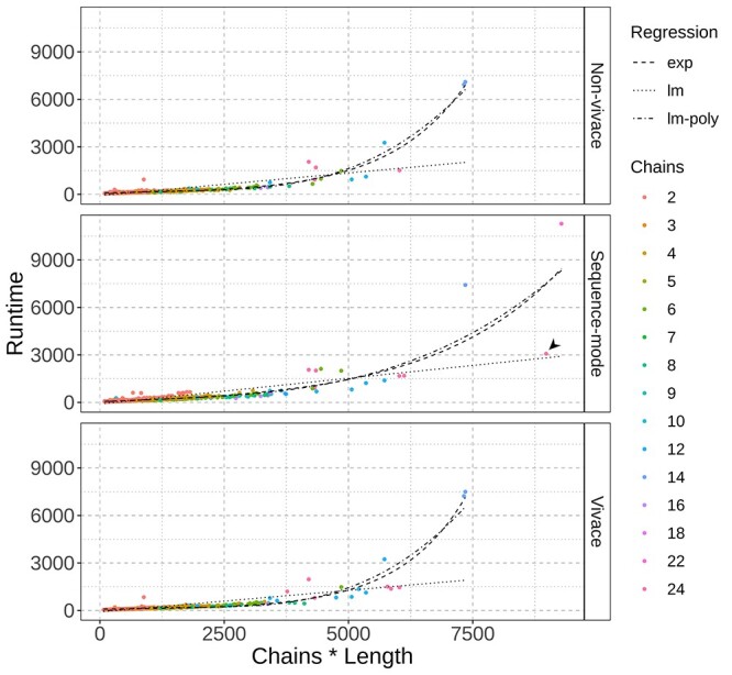
Runtimes calculated for each mode as a function of the complex size (i.e. the number of chains times the chain length). Linear (dotted lines), exponential (dashed lines) and polynomial (dot-dashed lines) models were fitted to the data points, with the exponential and polynomial models presenting the best fits (BIC of 67444.68, 63214.79 and 62760.13, respectively). The black arrowhead points to a unusually fast runtime mentioned in the main text.

It is worth mentioning that these tests were performed with the default multiprocessing method. Alternatively, the user might opt for using the single-core mode and exploit other parallelization methods and/or queueing systems that better suit their particular framework.

ProtCHOIR was able to process a total of 3394 protomers in ~87 h, which we consider a reasonable amount of time for the modelling of a large portion of an organism’s whole proteome. In the sequence-mode run, the time taken to finish the modelling of the proteome was ~27% higher (111 h) mainly because in sequence-mode, ProtCHOIR was able to generate a higher number of homo-oligomeric models as output (c.f. Figure 8A).

Conclusions

In this work, we described a novel pipeline tool, ProtCHOIR, which aims to build homo-oligomeric complexes from either protomeric structures or from protein sequences.

Although there have been important developments in oligomeric complexes modelling [42–44], there is still room for improvement in the throughput of most methods. The GalaxyHomomer server, for example, indicates upon submission that the average running time is between 6 and 12 h. The SwissModel server is considerably faster and has a very elegant interface but the method is not available for local, high throughput, modelling campaigns.

ProtCHOIR was developed with the intent of maximizing the execution performance so it can be applied to proteome-scale modelling campaigns in a reasonable amount of time. Furthermore, we also focused on a user-friendly experience to maximize usability and interpretability of the results. In this sense, the installation procedure has been kept as simple as possible, and it can be easily done through a standard python package manager, PIP. The subsequent initial database set-up and periodic updates can be accomplished via a single command-line instruction.

Regarding the output results, we intended to generate a comprehensive, easily interpretable, data-rich and visually appealing final report. That, along with the summary TSV file, allows for both protein-specific and large-scale analysis of the modelled proteins, which is one of the strong suits of our approach.

The most time-consuming tasks have been implemented under a multiprocessed framework, leading to much shorter execution times via a simple command-line option (–multiprocess). In spite of that, we also implemented a single-core version of the pipeline so it can be run under different hardware architectures. Our software also allows for automatic full or partial compression of the result files, which facilitates the handling of a larger volume of data.

As a proof-of-concept, we used a set of M. abscessus protomeric structures previously generated by our group to build homo-oligomeric structures in proteome-scale, which could be accomplished in about 3 or 4 days, depending on the execution mode.

We have also incorporated a convenience function to allow the construction of monomeric structures, which further increases the applicability and throughput of our tool. More ambitiously, we intend to incorporate the on-demand construction of hetero-oligomeric complexes and to develop an associated tool capable of predicting protein–protein complexes in a given proteome.

Overall, we believe ProtCHOIR will be of assistance in a number of structure-based studies involving, but not limited to, large-scale assessment of druggability, development of PPI inhibitors, virtual screening, molecular docking and dynamics, drug-target prospection and computer-aided drug development.

Additional information

Supplementary information is available for this paper.

Key Points

• We present ProtCHOIR, a python-based application that automates and streamlines the construction of homo-oligomeric complexes.

• ProtCHOIR presents high accuracy and is able to build models with the correct number of chains in over 90% of the cases.

• The pipeline is optimized for high-throughput modelling studies, and we show in a proof-of-concept run that it was able to process 2/3 of M. abscessus proteome (3405 proteins) in ~4 days.

Pedro H. M. Torres is a Professor of Bioinformatics and Biochemistry at the Federal University of Rio de Janeiro. He has a PhD degree in Biophysics and researches mainly in the field of protein modelling, molecular dynamics and computer-aided drug discovery.

Artur D. Rossi has bachelor’s degrees in computing engineering and in information technology and is MSc degree in computational modelling with focus on protein modelling and analysis.

Tom L. Blundell, Director of Research in Biochemistry, Cambridge, UK, is a structural and computational biologist with over 650 published research papers, H-factor 119, who has also developed new approaches to structure-guided fragment-based drug discovery.

Funding

Cystic Fibrosis Trust (RG 70975); Wellcome Trust Investigator Award, PHZJ/489 RG83114 (2016-2021) TLB thanks the Wellcome Trust for support through an Investigator Award (200814/Z/16/Z; 2016 -) to T.L.B.; Brazilian National Council for Scientific and Technological Development to P.H.M.T.

References

- 1. Mat-Sharani S, Quay DHX, Ng CL, et al. Structural genomics. In: Shoba Ranganathan, Michael Gribskov, Kenta Nakai, Christian SchShoba Ranganathan, Michael Gribskov, Kenta Nakai, Christian Schönbachnbach (eds.) Encyclopedia of Bioinformatics and Computational Biology: ABC of Bioinformatics, Cambridge, MA: Academic Press, 2018, 1–3. [Google Scholar]
- 2. Grabowski M, Niedzialkowska E, Zimmerman MD, et al. The impact of structural genomics: the first quindecennial. J Struct Funct Genomics 2016;17:1–16. [DOI] [PMC free article] [PubMed] [Google Scholar]
- 3. Levitt M. Nature of the protein universe. Proc Natl Acad Sci U S A 2009;106(27):11079–84. [DOI] [PMC free article] [PubMed] [Google Scholar]
- 4. Chen H, Engkvist O, Wang Y, et al. The rise of deep learning in drug discovery. Drug Discov Today 2018;23(6):1241–50. [DOI] [PubMed] [Google Scholar]
- 5. Baker D, Sali A. Protein structure prediction and structural genomics. Science (80- ) 2001;294(5540):93–6. [DOI] [PubMed] [Google Scholar]
- 6. Khor BY, Tye GJ, Lim TS, et al. General overview on structure prediction of twilight-zone proteins. Theor Biol Med Model 2015;12:1–11. [DOI] [PMC free article] [PubMed] [Google Scholar]
- 7. Dhingra S, Sowdhamini R, Cadet F, et al. A glance into the evolution of template-free protein structure prediction methodologies. Biochimie 2020;175:85–92. [DOI] [PubMed] [Google Scholar]
- 8. Fiser A. Comparative Protein Structure Modelling. In: From Protein Struct. to Funct. with Bioinforma, 2017, 91–134.
- 9. Becker D, Selbach M, Rollenhagen C, et al. Robust salmonella metabolism limits possibilities for new antimicrobials. Nature 2006;440(7082):303–7. [DOI] [PubMed] [Google Scholar]
- 10. Schmid MB. Do targets limit antibiotic discovery? Nat Biotechnol 2006;24(4):419–20. [DOI] [PubMed] [Google Scholar]
- 11. Pieper U, Webb BM, Dong GQ, et al. ModBase, a database of annotated comparative protein structure models and associated resources. Nucleic Acids Res 2014;42:1–11. [DOI] [PMC free article] [PubMed] [Google Scholar]
- 12. Lewis TE, Sillitoe I, Andreeva A, et al. Genome3D: a UK collaborative project to annotate genomic sequences with predicted 3D structures based on SCOP and CATH domains. Nucleic Acids Res 2013;41:499–507. [DOI] [PMC free article] [PubMed] [Google Scholar]
- 13. Lewis TE, Sillitoe I, Andreeva A, et al. Genome3D: exploiting structure to help users understand their sequences. Nucleic Acids Res 2015;43(D1):D382–6. [DOI] [PMC free article] [PubMed] [Google Scholar]
- 14. Ochoa-montano B, Mohan N, Blundell TL, et al. CHOPIN: a web resource for the structural and functional proteome of mycobacterium tuberculosis. Database (Oxford) 2015;2015:1–10. [DOI] [PMC free article] [PubMed] [Google Scholar]
- 15. Skwark MJ, Torres PHM, Copoiu L, et al. Mabellini: a genome-wide database for understanding the structural proteome and evaluating prospective antimicrobial targets of the emerging pathogen mycobacterium abscessus. Database 2019;2019:1–16. [DOI] [PMC free article] [PubMed] [Google Scholar]
- 16. Alsulami AF, Thomas SE, Jamasb AR, et al. SARS-CoV-2 3D database: understanding the coronavirus proteome and evaluating possible drug targets. Brief Bioinform 2021;1–12. [DOI] [PMC free article] [PubMed] [Google Scholar]
- 17. Bolanos-Garcia VM, Wu Q, Ochi T, et al. Spatial and temporal organization of multi-protein assemblies: achieving sensitive control in information-rich cell-regulatory systems. Philos Trans R Soc A Math Phys Eng Sci 2012;370(1969):3023–39. [DOI] [PubMed] [Google Scholar]
- 18. Chaplin AK, Blundell TL. Structural biology of multicomponent assemblies in DNA double-strand-break repair through non-homologous end joining. Curr Opin Struct Biol 2020;61:9–16. [DOI] [PubMed] [Google Scholar]
- 19. Kefala Stavridi A, Appleby R, Liang S, et al. Druggable binding sites in the multicomponent assemblies that characterise DNA double-strand-break repair through non-homologous end joining. Essays Biochem 2020;64(5):791–806. [DOI] [PMC free article] [PubMed] [Google Scholar]
- 20. Meyer MJ, Beltrán JF, Liang S, et al. Interactome INSIDER: a structural interactome browser for genomic studies. Nat Methods 2018;15(2):107–14. [DOI] [PMC free article] [PubMed] [Google Scholar]
- 21. Dey S, Ritchie DW, Levy ED. PDB-wide identification of biological assemblies from conserved quaternary structure geometry. Nat Methods 2018;15(1):67–72. [DOI] [PubMed] [Google Scholar]
- 22. Krissinel E, Henrick K. Inference of macromolecular assemblies from crystalline state. J Mol Biol 2007;372(3):774–97. [DOI] [PubMed] [Google Scholar]
- 23. Daily J. Parasail: SIMD C library for global, semi-global, and local pairwise sequence alignments. BMC Bioinformatics 2016;17:1–11. [DOI] [PMC free article] [PubMed] [Google Scholar]
- 24. Chapman BA, Chang JT. Biopython: python tools for computational biology. ACM SIGBIO Newsl 2000;20(2):15–9. [Google Scholar]
- 25. Cock PJA, Antao T, Chang JT, et al. Biopython: freely available python tools for computational molecular biology and bioinformatics. Bioinformatics 2009;25(11):1422–3. [DOI] [PMC free article] [PubMed] [Google Scholar]
- 26. Camacho C, Coulouris G, Avagyan V, et al. BLAST+: architecture and applications. BMC Bioinformatics 2009;10:1–9. [DOI] [PMC free article] [PubMed] [Google Scholar]
- 27. Suzek BE, Wang Y, Huang H, et al. UniRef clusters: a comprehensive and scalable alternative for improving sequence similarity searches. Bioinformatics 2015;31(6):926–32. [DOI] [PMC free article] [PubMed] [Google Scholar]
- 28. Altschul SF, Madden TL, Schäffer AA, et al. Gapped BLAST and PSI-BLAST:a new generation of protein database search programs. Nucleic Acids Res 1997;25(17):3389–402. [DOI] [PMC free article] [PubMed] [Google Scholar]
- 29. Tien MZ, Meyer AG, Sydykova DK, et al. Maximum allowed solvent accessibilites of residues in proteins. PLoS One 2013;8(11):e80635. [DOI] [PMC free article] [PubMed] [Google Scholar]
- 30. Wimley WC, White SH. Experimentally determined hydrophobicity scale for proteins at membrane interfaces. Nat Struct Biol 1996;3(10):842–8. [DOI] [PubMed] [Google Scholar]
- 31. Krogh A, Larsson B, Von Heijne G, et al. Predicting transmembrane protein topology with a hidden Markov model: application to complete genomes. J Mol Biol 2001;305(3):567–80. [DOI] [PubMed] [Google Scholar]
- 32. Chen VB, Arendall WB, Headd JJ, et al. MolProbity: all-atom structure validation for macromolecular crystallography. Acta Crystallogr Sect D Biol Crystallogr 2010;66(1):12–21. [DOI] [PMC free article] [PubMed] [Google Scholar]
- 33. Katoh K, Misawa K, Kuma K, et al. MAFFT: a novel method for rapid multiple sequence alignment based on fast Fourier transform. Nucleic Acids Res 2002;30(14):3059–66. [DOI] [PMC free article] [PubMed] [Google Scholar]
- 34. Capra JA, Singh M. Predicting functionally important residues from sequence conservation. Bioinformatics 2007;23(15):1875–82. [DOI] [PubMed] [Google Scholar]
- 35. Hunter JD. Matplotlib: a 2D graphics environment. Comput Sci Eng 2007;9(3):90–5. [Google Scholar]
- 36. Hagberg AA, Schult DA, Swart PJ.. Exploring network structure, dynamics, and function using NetworkX. In: 7th Annual Python in Science Conference (SciPy 2008), United States: Office of Scientific and Technical Information, 2008, pp. 11–5. [Google Scholar]
- 37. Krissinel E. Enhanced fold recognition using efficient short fragment clustering. J Mol Biochem 2012;1(2):76–85. [PMC free article] [PubMed] [Google Scholar]
- 38. Šali A, Blundell T. Comparative protein modelling by satisfaction of spatial restraints. J Mol Biol 1993;234(3):779–815. [DOI] [PubMed] [Google Scholar]
- 39. Henikoff S, Henikoff JG. Amino acid substitution matrices from protein blocks. Proc Natl Acad Sci U S A 1992;89(22):10915–9. [DOI] [PMC free article] [PubMed] [Google Scholar]
- 40. Fox NK, Brenner SE, Chandonia JM. SCOPe: structural classification of proteins - extended, integrating SCOP and ASTRAL data and classification of new structures. Nucleic Acids Res 2014;42:304–9. [DOI] [PMC free article] [PubMed] [Google Scholar]
- 41. Zhang Y, Skolnick J. TM-align: a protein structure alignment algorithm based on the TM-score. Nucleic Acids Res 2005;33(7):2302–9. [DOI] [PMC free article] [PubMed] [Google Scholar]
- 42. Baek M, Park T, Heo L, et al. GalaxyHomomer: a web server for protein homo-oligomer structure prediction from a monomer sequence or structure. Nucleic Acids Res 2017;45(W1):W320–4. [DOI] [PMC free article] [PubMed] [Google Scholar]
- 43. Bertoni M, Kiefer F, Biasini M, et al. Modeling protein quaternary structure of homo- and hetero-oligomers beyond binary interactions by homology. Sci Rep 2017;7:1–15. [DOI] [PMC free article] [PubMed] [Google Scholar]
- 44. Park H, Kim DE, Ovchinnikov S, et al. Automatic structure prediction of oligomeric assemblies using Robetta in CASP12. Proteins Struct Funct Bioinforma 2018;86:283–91. [DOI] [PMC free article] [PubMed] [Google Scholar]
Associated Data
This section collects any data citations, data availability statements, or supplementary materials included in this article.