Consensus clustering of single-cell RNA-seq data by enhancing network affinity

Abstract

Elucidation of cell subpopulations at high resolution is a key and challenging goal of single-cell ribonucleic acid (RNA) sequencing (scRNA-seq) data analysis. Although unsupervised clustering methods have been proposed for de novo identification of cell populations, their performance and robustness suffer from the high variability, low capture efficiency and high dropout rates which are characteristic of scRNA-seq experiments. Here, we present a novel unsupervised method for Single-cell Clustering by Enhancing Network Affinity (SCENA), which mainly employed three strategies: selecting multiple gene sets, enhancing local affinity among cells and clustering of consensus matrices. Large-scale validations on 13 real scRNA-seq datasets show that SCENA has high accuracy in detecting cell populations and is robust against dropout noise. When we applied SCENA to large-scale scRNA-seq data of mouse brain cells, known cell types were successfully detected, and novel cell types of interneurons were identified with differential expression of gamma-aminobutyric acid receptor subunits and transporters. SCENA is equipped with CPU + GPU (Central Processing Units + Graphics Processing Units) heterogeneous parallel computing to achieve high running speed. The high performance and running speed of SCENA combine into a new and efficient platform for biological discoveries in clustering analysis of large and diverse scRNA-seq datasets.

Introduction

The innovation of next-generation sequencing technology has brought great breakthroughs to biological research. As a prominent representative, single-cell ribonucleic acid (RNA) sequencing (scRNA-seq) can simultaneously measure expression levels of thousands of genes in thousands of cells and plays an important role in transcriptomics and disease studies [1, 2]. The scRNA-seq revolution has overcome many of the key limitations of bulk RNA-seq and provides the ability to monitor gene regulation, discover new cell types and track the developmental trajectories of thousands of single cells in an experiment [3]. scRNA-seq has been applied to a broad range of tissues, cell lines and disease samples to address fundamental biological research questions and better understand the mechanisms underlying disease development [4–8].

A core element of scRNA-seq transcriptome profile analysis is to cluster the cells to reveal cell types and infer cell lineages based on the transcriptomic relations among the cells [9]. In order to identify novel cell types, unsupervised clustering is of central importance to the analysis of scRNA-seq data [10, 11]. There are many unsupervised clustering tools available currently, such as SNN-Cliq [12], pcaReduce [13], CIDR [14], SINCERA [15], GiniClust [16], RaceID [17], SIMLR [18], SC3 [19], PhenoGraph [20], Seurat2/3 [21, 22] and SCANPY [23]. Several review articles have summarized and compared these tools [9, 10, 24, 25]. However, due to the complexity of the cell typing problem caused by high levels of technical noise from different protocols [26, 27] and a large number of zeros (zeros commonly make up >50% of the total estimated genes with expression, known as dropouts) in scRNA-seq data [28, 29], no clustering method performs well for all scRNA-seq datasets [30]. Dropout noise is usually produced by the low RNA capture rate, resulting in false zero counts of gene expression levels [27, 31–33]. Dropout noise will introduce inaccurate measurements of cell–cell similarity (such as Pearson correlation, Euclidean distance, etc.) and will eventually reduce the performance of clustering methods. GiniClust [16] and RaceID [17] (including updated versions GiniClust2, RaceID2 and RaceID3) only perform well for datasets containing rare cell types; SCANPY [23], Seurat2/3 [21, 22] and PhenoGraph [20] can handle large datasets but may not be as accurate for small datasets. SC3 [19] and pcaReduce [13] contain stochastic procedures and do not provide stable clustering results, especially for larger datasets [10].

As a preliminary step of unsupervised clustering, the purpose of feature selection (or dimension reduction) is to identify the most informative genes (top 500–2000 genes) from a genome-wide gene pool by computing either the expression level variance [21, 34] or deviance across all cells [35]. The most commonly used feature selection method is principal component analysis (PCA), which has been employed by SC3 [19], pcaReduce [13], CIDR [14], TSCAN [36], Seurat [21, 22], PhenoGraph [20], SCANPY [23], etc. Because of the high levels of dropouts and other experimental noise in scRNA-seq data, the cell–cell similarity constructed from these selected features cannot accurately capture the modularity among cells. Another key technical step of a clustering method is estimating the cluster numbers, which is absent for most of the scRNA-seq clustering methods. For example, -means clustering method requires prior knowledge of the number of clusters. Moreover, it is biased to identifying clusters of similar size and thus is not good at detecting rare cell types. PhenoGraph, Seurat and SCANPY used Louvain community detection method in detecting clusters but cannot perform as well for small datasets [37]. So far, only a limited number of tools, such as SINCERA [15], SC3 [19], SIMLR [18] and SNN-Cliq [12], can provide estimation of the cluster number in scRNA-seq data by using divergent strategies, such as P-value thresholds based on the distribution of eigenvalues of expression matrix (SC3), distance threshold (SINCERA) and graph-based clustering algorithm (SNN-Cliq). However, their estimation accuracy and/or running time stand to be improved [9, 38]. For example, a recent systematic comparison study of 13 clustering algorithms shows that SNN-Cliq tends to find considerable more clusters than real ground truth numbers in 10 of 12 tested datasets [38]. Meanwhile, four methods, SNN-Cliq [12], BISCUIT [39], BackSPIN [40] and RaceID [17], required an unacceptable amount of time or failed to run on datasets with more than 10 000 cells. Since the final cell typing outcomes are sensitive to the numbers of selected features, reduced dimensions and clustering strategy, new clustering methods are needed to perform effective feature selection and method-specific estimation of cluster number [38, 41], all while being robust against experimental noise, especially dropouts.

Based on these observations, we developed a novel unsupervised clustering tool Single-cell Clustering by Enhancing Network Affinity (SCENA) to identify the cell types in scRNA-seq data. To overcome the impact of dropout noise and improve accuracy, SCENA uses several optimal strategies, such as multiple feature sets selection, network affinity enhancement and consensus clustering. By applying this method to 13 datasets that were generated by using diverse scRNA-seq techniques, we found that SCENA is superior to other clustering algorithms in most of these datasets. In addition, the processing steps of SCENA are enhanced in parallel by using multiple process threads and/or the GPU (Graphics Processing Units) computing technique. The SCENA software easily scales to datasets with tens of thousands of cells, and its R package is freely available at https://github.com/shaoqiangzhang/SCENA.

Materials and methods

Methodology overview

The input data for SCENA are an expression matrix in which columns correspond to cells and rows correspond to genes/transcripts (called features). Suppose the set of cells is denoted by and the number of cells by . Each element represents the expression level of gene/transcript in cell . A workflow for SCENA is illustrated in Figure 1. First, a cell–cell similarity matrix was calculated by using a selected gene subset (feature gene set). SCENA then used a local affinity matrix to update the similarity matrix to enhance the similarity within each cell group and relatively weaken the similarity among cell groups. Spectral clustering [42] was used to cluster cells, where the cluster number was automatically estimated by the affinity propagation (AP) method [43]. To reduce the feature extraction errors caused by a single feature set, SCENA conducted multiple feature sets. Subsequently, each updated cell similarity matrix that was obtained from each feature set was clustered, and these clustering results were merged into a consensus matrix (Figure 1E and F). Finally, the cell types were obtained by clustering the consensus matrix. The details of SCENA steps are described as follows.

Figure 1 .

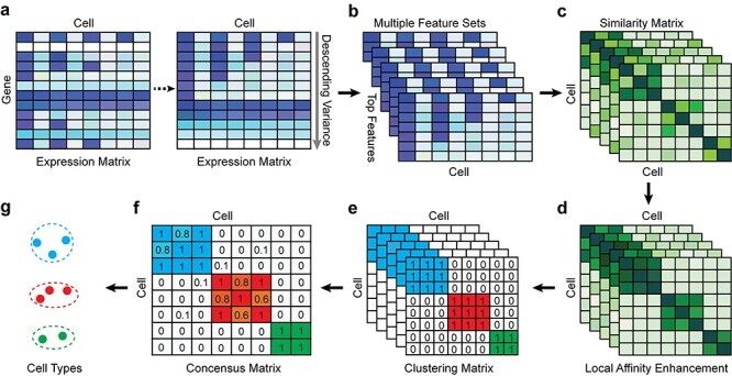
Illustrative example of SCENA steps. (A) Gene expression levels will be normalized and sorted by variances in descending order. (B) Multiple top feature gene sets are selected. (C) For each feature gene set, the cell–cell similarity matrix is constructed. (D) For each cell–cell similarity matrix, its local affinity is enhanced. (E) For each cell–cell similarity matrix, the number of clusters is estimated and clusters are detected by a spectral clustering method. (F) Consensus clustering matrix is calculated by merging the clustering results of multiple feature gene sets. (G) Cell populations are annotated for different clusters.

Data preprocessing and feature set selection

Three steps of preprocessing should be performed: gene filtering, data log-transformation and normalization. If a gene/transcript (called feature) has less than 5% of non-zero elements across cells in , the corresponding row is filtered out from . Meanwhile, if a feature has less than 5% zero elements across cells in , the corresponding row is also filtered out. Each element of the corresponding matrix is log-transformed after adding a pseudo-count of 1, that is, for each . Highly variable features are selected in this step. For each feature gene , its variance is calculated by

(1)

where is the mean value of features. All features are sorted by variance in descending order and the top feature genes are selected. Since it is hard to know how many top informative features can achieve the best clustering effect, a specific threshold (for example, the top 1000 informative genes) is often simply set based on experience. Here, instead of using a single feature set, we used multiple feature sets that include the top , top ,, and top feature genes. Based on performance evaluations of different feature sets , we select a combination of feature sets. After data analysis, each set of top features () generally does not exceed 5% of the total features in a dataset. For each selected feature , the z-score normalization is performed as , , where is the mean value of the feature and is the SD of the feature.

Constructing cell similarity matrices

For a set of top selected features, we preserve the feature rows to obtain a expression matrix . For any two cells , the Euclidean distance between and is computed. Here, the scaled exponential similarity kernel in SNF [44] is invoked to convert the Euclidean distance into a similarity score between each pair of cells:

(2)

where is the average values of Euclidean distances between and each of its -nearest neighbors (KNN). Then, a normalized cell similarity matrix of is constructed as follows:

(3)

The normalized similarity matrix is denoted by , which is an symmetric matrix and has . Meanwhile, a normalized local affinity matrix is constructed based on KNN:

(4)

where represents the set of and its KNN. Note that carries all the similarity information of each cell to all others, whereas only keeps information about of the most similar cells to enhance the local affinity for each cell. The selection of parameter of KNN is related to the number of cells. The default is set as 10 if , and = 20 if .

Local affinity enhancement

Given a set of selected features, we can construct similarity matricesusing equation (3) and using equation (4) for the th group of selected features, . In order to enhance the affinities of cells sharing KNN, the following formula with iterations is used:

(5)

which can ensure that similarity information is only propagated through the shared neighbors [44]. Since both and are normalized matrices, each element in will not be >1 in each iteration. Suppose that . The iterative process will be terminated if reaches a relatively stable state (i.e. for all and ) or if reaches a fixed upper number . The number of iterations that can result in the best and stable enhancement effect is related to the number . In practice, formula (5) can be reformed as , and can be obtained by iterations of matrix products. Additionally, if the number of cells , the upper number is set as 50; otherwise, is set as . Generally, the true number of iterations is below the upper number .

Estimate cluster number and spectral clustering

For each final matrix , we invoke normalized spectral clustering according to [45]，which first computes a normalized Laplacian where is defined as a diagonal matrix with the degrees (the total number of non-zero elements for each row of ) on the diagonal, then computes the first eigenvectors of to form a matrix and finally performs -means clustering on the row-normalized matrix of . Before running the spectral clustering, we use the AP method [43] to automatically estimate the number of clusters. An R package ‘APCluster’ [46] with the default parameters was employed in this step.

The final result of spectral clustering for each is saved as a (0,1)-matrix, , , in which 1 and 0, respectively, represent that the corresponding two cells are and are not grouped together (as shown in Figure 1E). In order to increase the speed of SCENA, for the given sets of selected features, threads are called for separately constructing matrices , and and for doing clustering on , .

Consensus clustering

Based on the matrices , a consensus matrix is constructed, where

(6)

The same as the previous step, spectral clustering is carried out on the consensus matrix to obtain the final clusters. For small datasets (<500 cells), the AP method is carried out on to re-estimate the number of clusters. For large datasets ( cells), in order to minimize the running time of the program, the median of in the previous step is taken as the input number of clusters of spectral clustering in this step.

Datasets and performance assessment

Thirteen publicly available scRNA-seq datasets derived from human and mouse cells (the detailed list in Table 1 and Supplementary Table S1 available online at http://bib.oxford-journals.org/) were used to evaluate the performances of SCENA versus other algorithms. Twelve datasets were downloaded from an online website (https://hemberg-lab.github.io/scRNA.seq.datasets/) and have been used previously to evaluate scRNA-seq clustering tools [19]. One big dataset with 24 822 cells was downloaded from NCBI GEO database with the access ID GSE124952 [47]. They range in size from dozens to tens of thousands of cells and are representative of datasets currently being published.

Table 1.

The number of clusters estimated by each tool on each dataset

Dataset	# Cells	# Cluster	SCENA	SC3	SNN-Cliq	SINCERA
Biase [58]	49	3	3	3	6	3
Treutlein [68]	80	5	3	3	3	19
Yan [69]	90	7	4	6	11	6
Goolam [70]	124	5	6	6	21	4
Ting [71]	149	7	7	10	13	10
Deng [72]	268	10	7	9	20	3
Pollen [49]	301	11	11	11	14	9
Patel [73]	430	5	8	17	25	10
Usoskin [50]	622	4/11a	4	11	20	11
Kolodziejczyk [57]	704	3	3	10	2	18
Klein [74]	2717	4	12	18	305	7
Zeisel [40]	3005	9	15	30	330	8
Bhattacherjee [47]	24 822	8	14	60	–	51

Notes: The datasets are listed in descending order of cell numbers. – Error reported or cannot process for the dataset with large number of cells

^aThis dataset has 4 big clusters and 11 subclusters

Adjusted Rand index (ARI) [48] is widely used in the evaluation of clustering on scRNA-seq data [9]. Given a predicted clustering and a true partition of objects (cells), the ARI is defined as follows:

(7)

where each represents the number of objects that are in both and , and and are the number of objects in and , respectively. Note that among the 13 datasets in Table 1, the 2 datasets of Pollen and Usoskin show multiple classifications of cell types in the corresponding literature [49, 50]. In the following experiments for the two datasets, the highest ARI score based on the different classifications of cell types is selected as the final score for each of the two datasets.

We estimated the time complexity of SCENA as , where is the total number of cells. The library ‘OpenBLAS’ (https://github.com/xianyi/OpenBLAS) is employed to accelerate matrix operations. To further speed up the SCENA algorithm, we also implemented the ‘gpuR’ GPU computing package for parallel matrix operations [51]. We ran SCENA on a Linux workstation (CPU: Intel Xeon E5-2620/2.10GHz/8 cores) with five threads and a GPU (GPU: Nvidia Tesla V100). We tested SCENA on the Bhattacherjee dataset that has a total of 24 822 cells [47]. To optimize the SCENA speed for large numbers of cells, we provided users a simplified version with iteration number for >6000 cells and for >10 000 cells.

To test the ability of detecting rare cell types, we did down-samplings of the Kolodziejczyk dataset that has three cell types with 295, 159 and 250 cells, respectively. For a cell type, we randomly selected certain number of cells (down-sampling number) and kept other two cell type numbers unchanged. We then ran SCENA on the down-sampled dataset and calculated the F1-score of the cluster that contains the most cells from the down-sampled cell type. F1-score is defined as , where (true positive) is the number of cells from the down-sampled cell type detected in the cluster, R is the cell number of the down-sampled cell type and is the cell number in the cluster. The down-sampling numbers of cells range from 10 to 70 in increments of 10. For each down-sampling number, the random selections for cell type were repeated 10 times, and the average F1-score was calculated.

Parameter setting and method comparison

All parameters in SCENA have default values, which are automatically set based on the number of cells and the total number of filtered features. In particular, a combination of five feature sets was selected from the top 5% of the total features sorted by variance in descending order. For example, if the total number of features is in a typical scRNA-seq dataset, five feature sets will be selected from the top 250 features. To reduce the combination complexity, we selected the top 50, top 100, top 150, top 200 and top 250 features as five different feature sets. In general, three kinds of combinations of the five feature sets were automatically set based on the total number of features: a combination (50, 100, 150, 200 and 250) for , a combination (50, 100, 200, 400 and 800) for and a combination (200, 400, 600, 800 and 1000) for . Default parameter values for the 13 experimental datasets are listed in Supplementary Table S2 available online at http://bib.oxfordjournals.org/.

To benchmark SCENA, we considered five popular tools: SC3 [19], Seurat3 [21, 22], SNN-Cliq [12], SINCERA [15] and pcaReduce [13]. A technical summary of these methods and software download links can be found in in Supplementary Table S3 available online at http://bib.oxfordjournals.org/. The gene filter was applied to all datasets (the last column in Supplementary Table S2 available online at http://bib.oxfordjournals.org/ is the number of filtered features). Data log-transformation and normalization were implemented by following the instructions of each tool accordingly. For example, SC3 performs log-transformation but not normalization, while SINCERA performs z-score normalization but not log-transformation. For all tools, we used the parameters according to the authors’ tutorials (see Supplementary File 1 available online at http://bib.oxfordjournals.org/ for command details). Specifically, the number of clusters for each tool was set as their automatically estimated number (if provided) or the best trained number for each dataset. SNN-Cliq was run using the parameter of KNN between 3 and 25 to select the best . For scRNA-seq datasets that were generated by quantitative scRNA-seq with unique molecular identifiers (UMIs), Seurat3 used an R package ‘sctransform’ to do normalization; and the LogNormalize parameter in Seurat3 was used for other datasets. In addition, since the results of SC3 and pcaReduce may be changed for different initial conditions, we ran both of them 100 times on each dataset and took the median of the ARI scores as the final performance value. Here, the number of 100 replicates is a user practical number in real applications.

Results

Local affinity enhancement improves clustering performance

To precisely identify cell clusters from scRNA-seq data, an important consideration is to reduce the negative effects of dropout noise. Instead of statistically estimating the proportions of dropout counts among the scRNA-seq data [52, 53], we reduced the dropout effects by enhancing the local cell–cell similarity within the same cell groups and consensus clustering for multiple feature sets. To accomplish this aim, the SCENA algorithm will first repeatedly update the cell–cell similarity matrix by the local affinity matrix (i.e. , ), where is iteration step and is the number of nearest cell neighbors. This process will result in an enhanced matrix in which nodes with strong similarity are connected by enhanced similarities, while nodes with weak similarity are connected by relatively lower similarities. Thus, cells in the same cluster will receive higher similarities, while cells across different clusters will have relatively lower similarities.

We evaluated the local affinity enhancement of clustering performance on 13 scRNA-seq datasets by calculating an ARI score [48] that is widely used in clustering analyses in the scRNA-seq data [9]. We tested different and/or numbers on four different size datasets and found the ARI scores generally increased with and/or (Figure 2A). Specifically, the ARI scores stabilize with 20 iterations and different numbers () for the Pollen dataset that has 301 cells. In the Usoskin and Kolodziejcyk dataset (622 and 704 cells, respectively), the ARI scores stabilized with 20 iterations with the larger numbers used () but required more iterations for smaller numbers (5 and 10). In the Klein dataset that has 2717 cells, it requires 100 iterations to reach stable ARI scores. The improvement of ARI scores with increased and/or on different datasets confirms that the local enhancement strategy can improve clustering results. To further demonstrate how this process updates similarity matrix , an example similarity matrix (Pollen dataset) with a different number of iteration steps is shown in Figure 2B. It can be observed that the grayscale values within each cluster increase and the separation among different clusters becomes increasingly clearer with an increasing number of matrix iterations. Therefore, the relative affinity among the same types of cells in the similarity matrix can be enhanced by the local affinity matrix which is constructed by KNN.

Figure 2 .

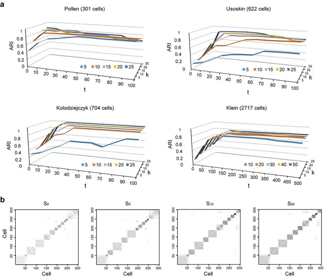
Testing SCENA performance for parameters and . (A) The ARI scores of the clustering results were obtained by varying values for of KNN and different number of matrix iterations for four datasets (top 200 highly variable features were used). (B) An example of local affinity enhancement with different numbers of iterations. is the original similarity matrix of Pollen’s dataset containing 301 cells, and the top 200 highly variable features were used. is the similarity matrix after the iteration. The dark dots indicate higher similarity scores between cell pairs.

The above results also show that the number of iterations and of KNN are correlated and both affected by the number of cells. We found that most of the ARI curves in Figure 2A can reach a relatively stable peak state, but note that some of them may fall back as the number of iterations increases, corresponding to over enhancement. Therefore, in order to prevent overfitting of cell similarities caused by an excessive number of iterations, the iterative operation in SCENA will be stopped if the difference of matrix is smaller than a given threshold (i.e. for all and ) or if reaches a fixed upper number. Meanwhile, we found that, for a smaller fixed , more iterative steps are required to reach the stable peaks. Therefore, the parameter cannot be too large or too small. In real application, we use fixed parameters with for small datasets () and for larger datasets (). In addition, for a fixed , the larger the dataset, the more iterations are required to reach the peak ARI score. Overall, we found from the experiments that when (), the SCENA algorithm can achieve a better effect if the upper number of iterations is set to 50 (); and with an increase in the number of cells, the corresponding upper number of iterations should also increase. When , the upper number of can be set to [/10] ().

Consensus clustering from multiple feature sets improves clustering performance

To define how many genes (features) are needed to calculate cell–cell similarity is another technical challenge in unsupervised single-cell clustering analysis. If we know in advance the marker genes for different cell types, higher clustering precision can be obtained. However, most single-cell RNA datasets have no such marker genes available. The most commonly used strategy for automatically selecting feature gene sets is PCA [35, 54–56] that usually selects the genes with larger contributions in the first component as feature genes. However, PCA was benchmarked to be time consuming and requires large amounts of memory for large-scale scRNA-seq datasets [56]. Furthermore, PCA on log-normalized UMI counts may lead to distorted low-dimensional factors and false discoveries of marker genes [35]. Since PCA is used as a preprocessing step in divergent methods, such as SC3, pcaReduce, CIDR, TSCAN, Seurat, PhenoGraph and SCANPY, it is a bottleneck for subsequent clustering analysis. Instead of using single feature gene sets predefined by PCA, we use multiple feature gene sets for parallel clustering and integrate the individual clustering results for a consensus clustering output.

We started by screening highly variable features from all genes/transcripts. For a given dataset, the SD of the logarithmic gene expression values in all cells was calculated. All genes/transcripts were then sorted by SD in descending order. On 12 datasets, we found the distribution curves of SDs are highly variable (Supplementary Figure S1A available online at http://bib.oxfordjournals.org/). For a given dataset, we then selected the right tail (with ~5% significance level) as its candidate gene pool. When different numbers of the top-ranked features with the largest variances were selected to do clustering analysis, we found that the performances under different numbers of top features are quite varied (Supplementary Figure S1B available online at http://bib.oxfordjournals.org/). For example, when more genes are selected in Biase dataset, the ARI scores keep increasing, while the ARI scores of the other four datasets show a tendency to decrease when more genes are selected. These observations show that feature genes are varied in different experiments and are affected by divergent biological conditions. To optimize the process of defining feature sets, we use multiple feature sets to do consensus clustering (see Materials and Methods for details). On 12 datasets, we found that most ARI scores from consensus clustering results were higher than those using a single feature set (Figure 3). Specifically, the consensus clustering results for nine datasets (Biase, Yan, Deng, Goolam, Patel, Pollen, Usoskin, Kolodziejczy and Treutlein) reached their highest ARI scores. Although consensus clustering results of other datasets (Ting, Klein and Zeisel) are not maximum with SCENA, the ARI differences are very small (mean = 0.026, SD = 0.009). Considering the large variances of ARI scores that are observed for the different feature sets used in the Treutlein, Yan, Goolam, Ting and Patel datasets, the consensus clustering based on multiple feature sets provides a stable strategy for precise clustering and avoids high variations that are calculated from a single feature set.

Figure 3 .

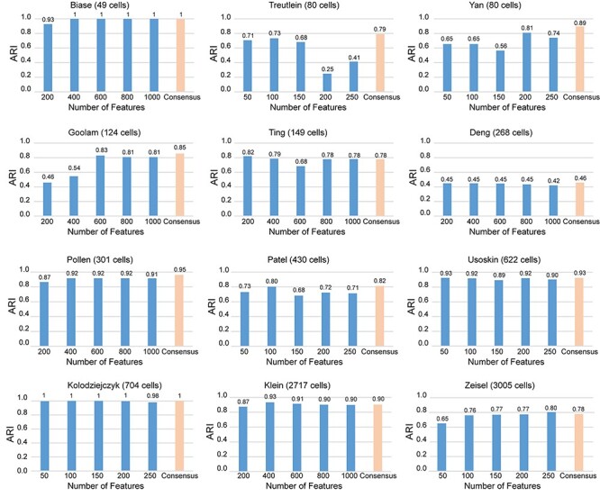
Comparisons of ARI scores for different feature sets. On 12 datasets, the ARI scores were calculated for five feature sets individually, and the consensus clustering results were based on the combination of five feature sets.

To further understand the advantage of multiple feature gene sets versus single feature gene set (top ranked or PCA selected), we ran SCENA by increasing the number of feature sets (Supplementary Figure S2A available online at http://bib.oxfordjournals.org/). For a single feature set , we first ran SCENA by using the PCA selected 30 features and top-50 ranked features, but no concordant results are observed in five tested datasets, e.g. the results from top-50-ranked features are better than PCA-based results in three datasets but are worse in the other two datasets. When more feature sets used, the performance increases when . When used, the ARI scores on the five datasets are all better than the single PCA-based results. However, we also observed that performance is disconcordant when , that is, the ARI scores on the two datasets continue to increase, whereas the scores on the other three datasets slightly decrease, indicating possible overfitting in consensus clustering. Taken together, these systematic evaluations confirmed that, compared to a single feature set (even for a PCA-estimated feature set), multiple feature sets improve the clustering performance. We suggest that is a practical value that is appropriate for most applications.

Performance comparison of SCENA and other methods

We compared the SCENA algorithm to five well-known algorithms on 12 benchmark datasets [9, 19] and the Bhattacherjee dataset that has a large number of 24 822 cells [47]. We ran these tools with default parameter settings (described in Materials and Methods section) and compared the ARI scores of clustering results for the 13 datasets (Figure 4, Supplementary Table S4 available online at http://bib.oxfordjournals.org/). First, we found that ARI scores derived from SCENA ranked first for nine datasets, while SC3 ranked first for three datasets and SINCERA ranked first for two datasets (here, SCENA and SINCERA ranked equal first for the Biase dataset). In particular, SCENA exhibited superior performance in smaller datasets [e.g. Biase (49 cells), Treutlein (80 cells), Yan (90 cells) and Goolam (123 cells)] and larger datasets [e.g. Usoskin (622 cells), Kolodziejczyk (704 cells), Klein (2717 cells), Zeisel (3005 cells) and Bhattacherjee (24 822 cells)]. While SC3 and SINCERA showed higher ARI scores for datasets of medium size [e.g. Ting (149 cells), Deng (268 cells), Pollen (301 cells) and Patel (365 cells)]. We note that the SEURAT method seems to not work well for small datasets [e.g. Biase (49 cells), Treutlein (80 cells) and Yan (90 cells)]; SC3 and SNN-Cliq cannot properly output results for the very large dataset Bhattacherjee (24 822 cells). Meanwhile, SCENA achieved ARI scores greater than 0.77 on the other 12 datasets (the exception being the Deng dataset), indicating good clustering performance on divergent datasets generated from different scRNA-seq techniques.

Figure 4 .

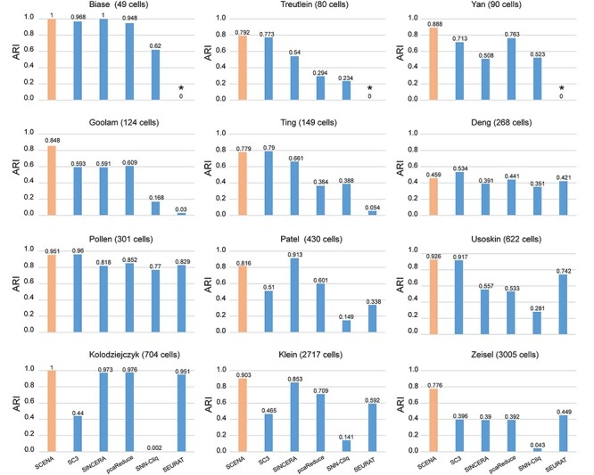
Performance comparisons of SCENA and the other five tools. The comparisons are based on ARI scores that were calculated by six tools on 12 datasets. For all tools, we used the default parameters according to the authors’ tutorials (please see Materials and Methods section for more details). *SEURAT can be used for small datasets with a size of less than 100 cells.

To systematically test the ability of these methods in detecting rare cell types (small cell numbers), we did down-samplings of the Kolodziejczyk dataset that has three cell types with 295, 159 and 250 cells, respectively. We calculated the F1-score that is defined as the balance between the recall and precision of clustering the down-sampled cells. F1-score ranges from 0 to 1, and a bigger score indicates a better precision-recall of cell type predictions. We found that, although the SCENA F1-scores are slightly less than SC3 F1-scores at 10 and 20 cell cases, they are better for the 30, 40, 50, 60 and 70 cell cases (>0.92, Supplementary Figure S2B available online at http://bib.oxfordjournals.org/). Among these six methods, four are deterministic, but SC3 and pcaReduce may output different results if different initializations are used. To check potential ARI variations, we ran clustering analyses 100 times for both SC3 and pcaReduce on the 12 datasets, respectively. We found that SC3 exhibited stable performance for seven datasets and showed variations of ARI scores on five relatively large datasets (Deng, Patel, Usoskin, Klein and Zeisel. Supplementary Figure S3A available online at http://bib.oxfordjournals.org/). Comparatively, pcaReduce showed larger variations for most of the 12 datasets (Supplementary Figure S3B available online at http://bib.oxfordjournals.org/).

As an unsupervised clustering method, SCENA can accept user-desired cluster numbers as input or can automatically estimate the possible numbers of cell clusters. Here, we compared the SCENA-estimated cluster numbers to the numbers that were provided by authors of previous studies based on marker genes or experimental conditions. After applying SCENA to the 13 datasets, we found that SCENA-estimated cluster numbers and the numbers of cell types labeled by the authors were similar (P-value = 0.17, chi-squared testing) and their differences were very small (mean = 2.17 and SD = 2.73, see Table 1). The mean difference obtained by SCENA was smaller than the results of the other three methods (SC3, SNN-Cliq and SINCERA) that can also estimate cluster numbers for 12 datasets (mean = 6.91 for SC3, mean = 118.19 for SNN-Cliq and mean = 5.17 for SINCERA). Therefore, SCENA performs better in estimating the number of clusters compared to the methods used in the other three tools.

Robustness against dropout noise and high speed of SCENA

To further demonstrate that SCENA can reduce the influence of dropouts, we tested it on the Kolodziejczyk dataset by artificially adding different percentages of dropout noise. The Kolodziejczyk dataset is suitable for such benchmark validation since it has a median size of 704 cells that clearly clustered into three groups [57]. Considering the dropouts are more likely generated for genes with low expression levels, we introduced dropout noise by setting different percentages of non-zero elements (UMI count <200) to zero. For each percentage, we produced 100 random replicates and calculated the medians of ARI scores for them. First, we observed SCENA continued to yield high ARI scores for small percentages of dropouts (10%, 20% and 30%) (Figure 5A). ARI scores decreased slightly (to 0.94) when the dropout percentage increased to 80%, achieving a small ratio change of 0.075 (0.06/0.8). Although the ARI decreased when all genes with UMI count less than 200 were set to zero, the value obtained remained relatively high (0.56), suggesting the genes with high UMIs still contribute cell-type specific information. Meanwhile, we repeated the analysis of artificial dropout noise for other four methods (SC3, pcaReduce, SEURAT and SINCERA) and confirmed that SCENA has the best performance among them (Figure 5A). These results indicate that SCENA is robust against the dropout noise.

Figure 5 .

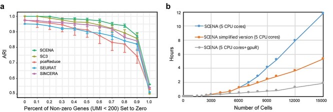
Robustness against dropout noise and running performance. (A) Performance comparisons of five methods on different percentages of artificial dropout noise added to the Kolodziejczyk dataset. (B) Time complexity of SCENA on different numbers of cells.

Since cell numbers in scRNA-seq studies have been increased from hundreds to thousands and even to tens of thousands, it is important to evaluate the performing time of clustering methods on different sample sizes. We implemented SCENA with parallel computing techniques by using multiple threads and GPU computing. We ran SCENA on the Bhattacherjee dataset [47] by sub-sampling up to 15 000 cells. Total processing time was no more than 50 s for a dataset of 1000 cells (Figure 5B). For a dataset of 3000 cells, the processing time was ~0.3 h which is practical. When SCENA was enabled by GPU computing, the matrix iterations for local affinity enhancement in the algorithm were parallelized by the ‘gpuR’ package [51]. When we ran the GPU computing version of SCENA on a GPU workstation, only 30 s of processing time was consumed for a dataset of 1000 cells and 9 min was consumed for a dataset of 3000 cells (Figure 5B). We further increased the cell numbers up to 15 000 cells and observed the high speed of SCENA. Specifically, SCENA successfully outputted the clustering results in ~1.2 h for 6000 cells, 4 h for 9000 cells, 8 h for 12 000 cells and 12 h for 15 000 cells. For large scRNA-seq datasets (>6000 cells), we further generated a simplified version by reducing the iteration numbers in affinity enhancement. SCENA can output results in ~2.5 h for 9000 cells, 3.7 h for 12 000 cells and 5.3 h for 15 000 cells. When a GPU is used, the running speed of SCENA is further dramatically reduced to less than 2 h even for even 15 000 cells. Overall, the testing results on different cell numbers show that SCENA has high speed in clustering tens of thousands of cells.

Detecting cell subpopulations from diverse scRNA-seq datasets

To evaluate SCENA’s ability to uncover known cell types and predict novel cell subpopulations, we present three real case studies, which represent small, medium and large numbers of cells. First, we applied SCENA to the Biase dataset [58] derived from for 49 mouse embryonic cells (9 1-Cells, 20 2-Cells 20 4-Cells) sequenced by the SMART-seq method. Results show that SCENA clearly detected a larger separation of the cells that are corresponding to the three embryonic stages (Figure 6A). Second, we applied SCENA to the Kolodziejczyk dataset derived from 704 mouse embryonic stem cells sequenced by the SMART-seq method [57]. These cells were cultured in three different conditions: serum, 2i and the alternative ground state a2i. We found that SCENA can separate these cells into three well-defined clusters, indicating distinct cellular transcriptomes of cells grown in different conditions.

Figure 6 .

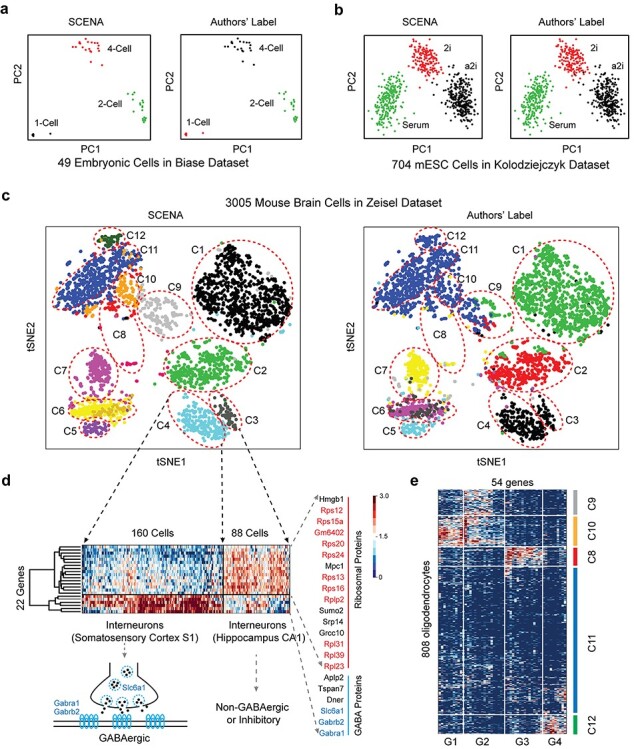
Application of SCENA to scRNA-seq datasets of different sizes. (A) Comparative analysis of clustering results on Biase dataset (small size). There are 49 embryonic cells for three groups as 1-cell, 2-cell and 4-cell types. (B) Comparative analysis of clustering results on the Kolodziejczyk dataset (medium size). There are 704 mESC cells that were cultured using three different conditions. (C) Comparative analysis of clustering results on Zeisel dataset (large size). A total of 3005 mouse brain cells were defined as 15 clusters by SCENA (left). Nine clusters were previously labeled by the authors (right). Twelve clusters (C1–C12) are annotated and indicated by red dot circles for comparative analysis. (D) Twenty-two genes with differential expression profiles in C3 and C4 clusters. Enriched ribosomal genes are marked in red. GABAergic related genes are marked in light blue. The detailed genes and cell information are listed in Supplementary Table S5 available online at http://bib.oxfordjournals.org/. (E) Fifty-four genes (in four sets G1, G2, G3, G4) with differential expression profiles in five clusters (C8, C9, C10, C11, C12). The detailed genes and cell information are listed in Supplementary Table S6 available online at http://bib.oxfordjournals.org/.

As a representative of large scRNA-seq datasets, we analyzed the SCENA results from the analysis of the Zeisel dataset that was sequenced by quantitative scRNA-seq with UMI. This dataset includes 3005 cells that were obtained from two regions of mouse brain: the primary somatosensory cortex (S1) and the hippocampal CA1 region [40]. Previous analyses have classified cells in S1 and CA1 as pyramidal neurons, interneurons, oligodendrocytes, astrocytes, microglia, vascular endothelial cells, mural cells and ependymal cells. On this complicated dataset, SCENA defined a total of 15 clusters that have clear boundaries and functional annotations (Figure 6C). First, we found the majority of SCENA clusters were consistent with the authors’ labels. As shown in Figure 6C, eight SCENA clusters show a high degree of overlap with the clusters annotated by original labels, including C1, C2, C4, C5, C6, C7 and C11. In particular, this overlap can be clearly observed for the C6 cluster that includes the two cell types projected by the tSNE method [59]. Second, we noticed that most of SCENA clusters provided more clear boundaries than those generated from original labels. In SCENA’s results of C2, C7 and C9, the cells can be clearly observed as local clusters, exhibiting local areas with high density. In particular, SCENA clustered C9 as a unique cluster that includes outlier points from three groups in original labels (Figure 6C). Meanwhile, any cells originally labeled as C1 can be found in C2 and C9 clusters. Third, we found that SCENA reported several new clusters by dividing large original clusters into smaller subclusters that have observable boundaries between them. For example, SCENA took C3 and C4 as two different cell types corresponding to two separable shapes between them. Meanwhile, SCENA separated C8, C9, C10, C11 and C12 from a single large cluster which was previously annotated by authors [40].

Fourth, we checked the differentially expressed genes for these clusters: C3, C4, C8, C9, C10, C11 and C12. As shown in Figure 6D, we found 20 genes with significantly different expression levels between clusters C3 and C4 (KS testing, P-values < 0.001), indicating functional classification of two cell types. Among these genes, 16 genes show higher expression in C3, and six show higher expression in C4 (Supplementary Table S5 available online at http://bib.oxfordjournals.org/). Interestingly, we found 11 ribosomal genes highly expressed in interneurons of hippocampus CA1, while three genes that are related to the neurotransmitter gamma-aminobutyric acid (GABA) were highly expressed in the interneurons of somatosensory cortex S1. The specific expression pattern of GABA receptor subunits (Gabra1 and Gabrb1) and transporter (Slc6a1) provide molecular evidence of GABAergic pathways in the interneurons of somatosensory cortex S1 [60]. For clusters C8, C9, C10, C11 and C12, we found at least four gene sets that showed differential expression profiles among them (red blocks in Figure 6E, detailed information in Supplementary Table S6 available online at http://bib.oxfordjournals.org/). Each gene set was shown to be significantly expressed in at least two cell clusters (KS testing, P-value < 0.001). In summary, these detailed clustering results show that SCENA can precisely define cluster numbers from datasets of various sizes generated from different scRNA-seq protocols and is able to detect individual cell types with different biological functions.

Discussion

The success of SCENA can be mainly attributed to three aspects. First, and maybe most importantly, SCENA exploits the local modularity of cells by enhancing the affinity among them. Since dropout noise and other experimental noise may falsely reduce or improve the relationship among same-cell groups, this iterative enhancement of local connections within individual modules will concordantly synchronize their similarities and enhance the differences between cell groups. Second, it uses diverse feature sets. This strategy helps to avoid the usage limitation of a single feature set. In contrast, many previous methods consider only one feature set that is selected by the PCA or tSNE. Third, SCENA takes the advantage of consensus clustering by merging several cluster results based on different feature sets. The combination of these three aspects makes SCENA robust to dropout noise and minimizes the impact of false positives and false negatives in cell–cell connections.

Compared with supervised methods that use predefined marker genes or geometric/conditional features of certain cell types, SCENA has an advantage in detecting novel cell types. Supervised clustering methods usually use prior knowledge of cell-type marker genes to annotate scRNA-seq data into predefined cell types [61–63]. Although these methods can reduce the burden of estimating features of cell types, the methods are unlikely to discover new cell types. Additionally, since known marker genes are very limited for many cell types, and some less studied types of cells even have no known marker genes, false negative results are more likely to be produced. SCENA can automatically estimate the cluster numbers based on the network connectome information and thus avoid the false labeling of outlier points. As a demonstration, we found that SCENA clusters in the Zeisel dataset show clear boundaries and higher local aggregations compared to other methods. Consequently, the detailed analysis of feature genes for 15 cell clusters provides potential marker gene sets for defining the molecular barcodes of these cell types. We especially checked two clusters with differential expression profiles of GABAergic-related genes that are highly expressed in the interneurons of the somatosensory cortex S1 but not in the hippocampus CA1 interneurons. Since various classes of cortical and hippocampal interneurons are putatively involved in the pathogenesis of the epilepsy [64–67], these single-cell-based analyses provide multimodal cell features in understanding the appropriate granularity of neuron types and potential functional abnormalities in epileptic brain.

Although SCENA achieved high performance in analyzing 13 datasets that were generated from diverse scRNA-seq protocols, there are several technical considerations in application. One general concern is the potential confounding factor in batch effects. In these 13 datasets, the cell populations were either known or were considered to be identical across batches. However, large-scale scRNA-seq datasets may be produced in different laboratories, at different times, by differing handling personnel and technology platforms, resulting in large variations or batch effects. Unlike dropout noise that generated by the stochasticity of gene expression, or by the failure in RNA library preparation [28, 29], batch effects can be highly nonlinear, making it difficult to separate them from biological variations. For example, the cells from different batches may introduce false modules within which the cells will achieve pseudo-similarity of expression patterns. In this case, additional normalization techniques must be applied to adjust the mean and variance of the gene expression, especially for heterogeneous datasets merged from different scRNA-seq methods, such as UMI or whole gene-body-based methods. Another possible concern is over the enhancement of local affinity since too many steps of enhancement may introduce over-diffused connections among cells, resulting in false cluster numbers. To avoid this, we comprehensively analyzed two parameters: the iteration step and the number of nearest cell neighbors . We empirically optimized them by considering the total cell numbers and potential cluster numbers. We suggest users not to use too many steps or too large a number of cell neighbors to avoid such over-enhancement. Another factor that may cause overfitting of SCENA is the number of feature sets, , where the ARI scores can be observed to be slightly lower on several datasets when (Supplementary Figure S2A available online at http://bib.oxfordjournals.org/). Therefore, we suggest the number of feature sets to be set as in practice. Since the gene features with high variance are considered to be good feature candidates, we selected the features for each of five feature sets only within top-ranked features with certain increments. In practice, we suggest the five feature sets to be (50, 100, 150, 200 and 250) for datasets with a smaller number of total gene features () and to be (200, 400, 600, 800, 1000) for the dataset with a larger number of total gene features (). These practical selections of multiple feature sets can highlight the major features, retain reasonable coverage and simplify the feature selection process that is usually time consuming. In the SCENA software, all these parameters will be automatically recommended and printed for users but will also be adjustable for user preference. Another general point to be considered in the clustering analysis of scRNA-seq data is the diversity of scRNA-seq techniques. Usually, the clustering analysis is started from a gene-cell expression matrix. Since there are more than 20 different scRNA-seq protocols available now [26, 27], specific normalization and preprocessing of the different protocols are essential for following clustering analysis and differential expression analysis.

In summary, SCENA is designed to reduce the effects of dropout noise, reconstruct cell–cell similarity and detect the biological variabilities across cells. SCENA is scalable to dataset size and works well on diverse datasets that are generated by different protocols. Considering scRNA-seq experiments are generating increased cell throughput and larger datasets, we equipped SCENA with a CPU + GPU heterogeneous parallel computing design and provided users with computing flexibility in analyzing relatively large datasets. Altogether, SCENA is tested to be an effective clustering method and may be useful in various fields of biological research by facilitating novel discoveries in the scRNA-seq data.

Key Points

• Clustering analysis is essential to identify novel cell types, gene expression patterns and marker genes.

• SCENA R package provides an effective platform for clustering analyses of scRNA-seq data.

• SCENA is robust against high dropout noise levels.

• SCENA is parallelized and easily scales to datasets with tens of thousands of cells.

Yaxuan Cui is a PhD D candidate at the College of Computer and Information Engineering, Tianjin Normal University, China. His research interests focus on bioinformatics and machine learning.

Shaoqiang Zhang is a professor at the College of Computer and Information Engineering, Tianjin Normal University, China. He received his PhD degree in operations research from Shandong University, Shandong, China. His research interests include bioinformatics, combinatorial optimization and high-performance computing. He is a member of IEEE and The China Computer Federation.

Ying Liang is an assistant professor at the College of Computer and Information Engineering, Tianjin Normal University, China. She received MS and PhD degrees from Harbin Engineering University, Heilongjiang, China. Her research interests include bioinformatics and machine learning.

Xiangyun Wang is an assistant professor at the College of Computer and Information Engineering, Tianjin Normal University, China. She received PhD degree from Beijing University of Aeronautics and Astronautics, Beijing, China. Her research interests include bioinformatics and machine learning.

Thomas N. Ferraro is a professor in the Department of Biomedical Sciences at CMSRU. Dr Ferraro earned his PhD in pharmacology from Thomas Jefferson University in Philadelphia (1985) and is recognized internationally as an expert in neuroscience and genetics. Dr Ferraro has published over 100 peer-reviewed scientific research papers. Current projects involve genetic mouse models of epilepsy, opioid addiction and neurodevelopmental disorders, such as Rett Syndrome. He is serving as the chairperson of an NIH advisory panel on Research Training and Career Development (since 2008) and is serving as a research consultant to the Veterans Affairs Medical Center in Coatesville PA (since 1990).

Yong Chen is an assistant professor in the Department of Molecular and Cellular Biosciences at Rowan University. Dr Chen is a bioinformatician and a computational biologist and has published over 40 peer-reviewed scientific research papers. His research interests include single cell omics data analysis, cancer epigenetics and neuroscience.

Authors’ contributions

S.Z. and Y.C. initiated the concept and supervised the study and designed the methodology. Y.C. implemented the software. Y.C., S.Z., Y.L., X.W. and Y.C. performed the data analysis. S.Z., Y.C. and T.N.F. drafted and reviewed the paper. All authors have read and approved the final manuscript.

Data availability

The source code and R package are freely available at https://github.com/shaoqiangzhang/SCENA. The datasets used in this study can be found at https://github.com/shaoqiangzhang/scRNAseq_Datasets.

Funding

Natural Science Foundation of Tianjin City (19JCZDJC35100); National Science Foundation of China (61572358 to S.Z.); Rowan University Startup grant (2019 for Y.C.).

References

- 1. Han Y, Gao S, Muegge K, et al. Advanced applications of RNA sequencing and challenges. Bioinform Biol Insights 2015;9(Suppl 1):29–46. [DOI] [PMC free article] [PubMed] [Google Scholar]
- 2. Stuart T, Satija R. Integrative single-cell analysis. Nat Rev Genet 2019;20(5):257–72. [DOI] [PubMed] [Google Scholar]
- 3. Trapnell C. Defining cell types and states with single-cell genomics. Genome Res 2015;25(10):1491–8. [DOI] [PMC free article] [PubMed] [Google Scholar]
- 4. Rozenblatt-Rosen O, Stubbington MJT, Regev A, et al. The human cell atlas: from vision to reality. Nature 2017;550(7677):451–3. [DOI] [PubMed] [Google Scholar]
- 5. Han X, Wang R, Zhou Y, et al. Mapping the mouse cell atlas by microwell-Seq. Cell 2018;172(5):1091–1107.e17. [DOI] [PubMed] [Google Scholar]
- 6. Reid AJ, Talman AM, Bennett HM, et al. Single-cell RNA-seq reveals hidden transcriptional variation in malaria parasites. Elife 2018;7:e33105. doi: 10.7554/eLife.33105. [DOI] [PMC free article] [PubMed] [Google Scholar]
- 7. Davie K, Janssens J, Koldere D, et al. A single-cell transcriptome atlas of the aging Drosophila brain. Cell 2018;174(4):982–998.e20. [DOI] [PMC free article] [PubMed] [Google Scholar]
- 8. Cusanovich DA, Reddington JP, Garfield DA, et al. The cis-regulatory dynamics of embryonic development at single-cell resolution. Nature 2018;555(7697, 7697):538–42. [DOI] [PMC free article] [PubMed] [Google Scholar]
- 9. Petegrosso R, Li Z, Kuang R. Machine learning and statistical methods for clustering single-cell RNA-sequencing data. Brief Bioinform 2020;21(4):1209–23. [DOI] [PubMed] [Google Scholar]
- 10. Kiselev VY, Andrews TS, Hemberg M. Challenges in unsupervised clustering of single-cell RNA-seq data. Nat Rev Genet 2019;20(5):273–82. [DOI] [PubMed] [Google Scholar]
- 11. Dijk D, Sharma R, Nainys J, et al. Recovering gene interactions from single-cell data using data diffusion. Cell 2018;174(3):716–729.e27. [DOI] [PMC free article] [PubMed] [Google Scholar]
- 12. Xu C, Su Z. Identification of cell types from single-cell transcriptomes using a novel clustering method. Bioinformatics 2015;31(12):1974–80. [DOI] [PMC free article] [PubMed] [Google Scholar]
- 13. Zurauskiene J, Yau C. pcaReduce: hierarchical clustering of single cell transcriptional profiles. BMC Bioinformatics 2016;17(1):140. [DOI] [PMC free article] [PubMed] [Google Scholar]
- 14. Lin P, Troup M, Ho JW. CIDR: ultrafast and accurate clustering through imputation for single-cell RNA-seq data. Genome Biol 2017;18(1):59. [DOI] [PMC free article] [PubMed] [Google Scholar]
- 15. Guo M, Wang H, Potter SS, et al. SINCERA: a pipeline for single-cell RNA-Seq profiling analysis. PLoS Comput Biol 2015;11(11):e1004575. [DOI] [PMC free article] [PubMed] [Google Scholar]
- 16. Jiang L, Chen H, Pinello L, et al. GiniClust: detecting rare cell types from single-cell gene expression data with Gini index. Genome Biol 2016;17(1):144. [DOI] [PMC free article] [PubMed] [Google Scholar]
- 17. Grün D, Lyubimova A, Kester L, et al. Single-cell messenger RNA sequencing reveals rare intestinal cell types. Nature 2015;525(7568):251–5. [DOI] [PubMed] [Google Scholar]
- 18. Wang B, Zhu J, Pierson E, et al. Visualization and analysis of single-cell RNA-seq data by kernel-based similarity learning. Nat Methods 2017;14(4):414–6. [DOI] [PubMed] [Google Scholar]
- 19. Kiselev VY, Kirschner K, Schaub MT, et al. SC3: consensus clustering of single-cell RNA-seq data. Nat Methods 2017;14(5):483–6. [DOI] [PMC free article] [PubMed] [Google Scholar]
- 20. Levine JH, Simonds EF, Bendall SC, et al. Data-driven phenotypic dissection of AML reveals progenitor-like cells that correlate with prognosis. Cell 2015;162(1):184–97. [DOI] [PMC free article] [PubMed] [Google Scholar]
- 21. Butler A, Hoffman P, Smibert P, et al. Integrating single-cell transcriptomic data across different conditions, technologies, and species. Nat Biotechnol 2018;36(5):411–20. [DOI] [PMC free article] [PubMed] [Google Scholar]
- 22. Stuart T, Butler A, Hoffman P, et al. Comprehensive integration of single-cell data. Cell 2019;177(7):1888–1902.e21. [DOI] [PMC free article] [PubMed] [Google Scholar]
- 23. Wolf FA, Angerer P, Theis FJ. SCANPY: large-scale single-cell gene expression data analysis. Genome Biol 2018;19(1):15. [DOI] [PMC free article] [PubMed] [Google Scholar]
- 24. Shekhar K, Menon V. Identification of cell types from single-cell transcriptomic data. Methods Mol Biol 2019;1935:45–77. [DOI] [PubMed] [Google Scholar]
- 25. Chen G, Ning B, Shi T. Single-cell RNA-Seq technologies and related computational data analysis. Front Genet 2019;10:317. [DOI] [PMC free article] [PubMed] [Google Scholar]
- 26. Haque A, Engel J, Teichmann SA, et al. A practical guide to single-cell RNA-sequencing for biomedical research and clinical applications. Genome Med 2017;9(1):75. [DOI] [PMC free article] [PubMed] [Google Scholar]
- 27. Mereu E, Lafzi A, Moutinho C, et al. Benchmarking single-cell RNA-sequencing protocols for cell atlas projects. Nat Biotechnol 2020;38(6):747–55. [DOI] [PubMed] [Google Scholar]
- 28. Kharchenko PV, Silberstein L, Scadden DT. Bayesian approach to single-cell differential expression analysis. Nat Methods 2014;11(7):740–2. [DOI] [PMC free article] [PubMed] [Google Scholar]
- 29. Tran HTN, Ang KS, Chevrier M, et al. A benchmark of batch-effect correction methods for single-cell RNA sequencing data. Genome Biol 2020;21(1):12. [DOI] [PMC free article] [PubMed] [Google Scholar]
- 30. Andrews TS, Hemberg M. M3Drop: dropout-based feature selection for scRNASeq. Bioinformatics 2019;35(16):2865–7. [DOI] [PMC free article] [PubMed] [Google Scholar]
- 31. Vieth B, Parekh S, Ziegenhain C, et al. A systematic evaluation of single cell RNA-seq analysis pipelines. Nat Commun 2019;10(1):4667. [DOI] [PMC free article] [PubMed] [Google Scholar]
- 32. Zhang MJ, Ntranos V, Tse D. Determining sequencing depth in a single-cell RNA-seq experiment. Nat Commun 2020;11(1):774. [DOI] [PMC free article] [PubMed] [Google Scholar]
- 33. Ziegenhain C, Vieth B, Parekh S, et al. Comparative analysis of single-cell RNA sequencing methods. Mol Cell 2017;65(4):631–643.e4. [DOI] [PubMed] [Google Scholar]
- 34. Brennecke P, Anders S, Kim JK, et al. Accounting for technical noise in single-cell RNA-seq experiments. Nat Methods 2013;10(11):1093–5. [DOI] [PubMed] [Google Scholar]
- 35. Townes FW, Hicks SC, Aryee MJ, et al. Feature selection and dimension reduction for single-cell RNA-Seq based on a multinomial model. Genome Biol 2019;20(1):295. [DOI] [PMC free article] [PubMed] [Google Scholar]
- 36. Ji Z, Ji H. TSCAN: pseudo-time reconstruction and evaluation in single-cell RNA-seq analysis. Nucleic Acids Res 2016;44(13):e117. [DOI] [PMC free article] [PubMed] [Google Scholar]
- 37. Fortunato S, Barthelemy M. Resolution limit in community detection. Proc Natl Acad Sci USA 2007;104(1):36–41. [DOI] [PMC free article] [PubMed] [Google Scholar]
- 38. Li R, Guan J, Zhou S. Single-cell RNA-seq data clustering: a survey with performance comparison study. J Bioinform Comput Biol 2020;18(04):2040005. [DOI] [PubMed] [Google Scholar]
- 39. Prabhakaran S, Azizi E, Carr A, et al. Dirichlet process mixture model for correcting technical variation in single-cell gene expression data. JMLR Workshop Conf Proc 2016;48:1070–9. [PMC free article] [PubMed] [Google Scholar]
- 40. Zeisel A, Munoz-Manchado AB, Codeluppi S, et al. Brain structure. Cell types in the mouse cortex and hippocampus revealed by single-cell RNA-seq. Science 2015;347(6226):1138–42. [DOI] [PubMed] [Google Scholar]
- 41. Qi R, Ma A, Ma Q, et al. Clustering and classification methods for single-cell RNA-sequencing data. Brief Bioinform 2020;21(4):1196–208. [DOI] [PMC free article] [PubMed] [Google Scholar]
- 42. Park S, Zhao H. Spectral clustering based on learning similarity matrix. Bioinformatics 2018;34(12):2069–76. [DOI] [PMC free article] [PubMed] [Google Scholar]
- 43. Frey BJ, Dueck D. Clustering by passing messages between data points. Science 2007;315(5814):972–6. [DOI] [PubMed] [Google Scholar]
- 44. Wang B, Mezlini AM, Demir F, et al. Similarity network fusion for aggregating data types on a genomic scale. Nat Methods 2014;11(3):333–7. [DOI] [PubMed] [Google Scholar]
- 45. John CR, Watson D, Barnes MR, et al. Spectrum: fast density-aware spectral clustering for single and multi-omic data. Bioinformatics 2020;36(4):1159–66. [DOI] [PMC free article] [PubMed] [Google Scholar]
- 46. Bodenhofer U, Kothmeier A, Hochreiter S. APCluster: an R package for affinity propagation clustering. Bioinformatics 2011;27(17):2463–4. [DOI] [PubMed] [Google Scholar]
- 47. Bhattacherjee A, Djekidel MN, Chen R, et al. Cell type-specific transcriptional programs in mouse prefrontal cortex during adolescence and addiction. Nat Commun 2019;10(1):4169. [DOI] [PMC free article] [PubMed] [Google Scholar]
- 48. Hubert L, Arabie P. Comparing partitions. Journal of Classification 1985;2(1):193–218. [Google Scholar]
- 49. Pollen AA, Nowakowski TJ, Shuga J, et al. Low-coverage single-cell mRNA sequencing reveals cellular heterogeneity and activated signaling pathways in developing cerebral cortex. Nat Biotechnol 2014;32(10):1053–8. [DOI] [PMC free article] [PubMed] [Google Scholar]
- 50. Usoskin D, Furlan A, Islam S, et al. Unbiased classification of sensory neuron types by large-scale single-cell RNA sequencing. Nat Neurosci 2015;18(1):145–53. [DOI] [PubMed] [Google Scholar]
- 51. Rupp K, Tillet P, Rudolf F, et al. ViennaCL-linear algebra library for multi- and many-core architectures. SIAM J Sci Comput 2016;38(5):S412–39. [Google Scholar]
- 52. Zhu L, Lei J, Devlin B, et al. A unified statistical framework for single cell and bulk Rna sequencing data. Ann Appl Stat 2018;12(1):609–32. [DOI] [PMC free article] [PubMed] [Google Scholar]
- 53. Li WV, Li JJ. An accurate and robust imputation method scImpute for single-cell RNA-seq data. Nat Commun 2018;9(1):997. [DOI] [PMC free article] [PubMed] [Google Scholar]
- 54. Kotliar D, Veres A, Nagy MA, et al. Identifying gene expression programs of cell-type identity and cellular activity with single-cell RNA-Seq. Elife 2019;8:e43803. doi: 10.7554/eLife.43803. [DOI] [PMC free article] [PubMed] [Google Scholar]
- 55. Wu Z, Shou L, Wang J, et al. Identification of the key gene and pathways associated with osteoarthritis via single-cell RNA sequencing on synovial fibroblasts. Medicine (Baltimore) 2020;99(33):e21707. [DOI] [PMC free article] [PubMed] [Google Scholar]
- 56. Tsuyuzaki K, Sato H, Sato K, et al. Benchmarking principal component analysis for large-scale single-cell RNA-sequencing. Genome Biol 2020;21(1):9. [DOI] [PMC free article] [PubMed] [Google Scholar]
- 57. Kolodziejczyk AA, Kim JK, Tsang JC, et al. Single cell RNA-sequencing of pluripotent states unlocks modular transcriptional variation. Cell Stem Cell 2015;17(4):471–85. [DOI] [PMC free article] [PubMed] [Google Scholar]
- 58. Biase FH, Cao X, Zhong S. Cell fate inclination within 2-cell and 4-cell mouse embryos revealed by single-cell RNA sequencing. Genome Res 2014;24(11):1787–96. [DOI] [PMC free article] [PubMed] [Google Scholar]
- 59. Maaten L, Hinton G. Visualizing high-dimensional data using t-SNE. JMLR 2008;9:2779–605. [Google Scholar]
- 60. Lim L, Mi D, Llorca A, et al. Development and functional diversification of cortical interneurons. Neuron 2018;100(2):294–313. [DOI] [PMC free article] [PubMed] [Google Scholar]
- 61. Zhang AW, O'Flanagan C, Chavez EA, et al. Probabilistic cell-type assignment of single-cell RNA-seq for tumor microenvironment profiling. Nat Methods 2019;16(10):1007–15. [DOI] [PMC free article] [PubMed] [Google Scholar]
- 62. Pliner HA, Shendure J, Trapnell C. Supervised classification enables rapid annotation of cell atlases. Nat Methods 2019;16(10):983–6. [DOI] [PMC free article] [PubMed] [Google Scholar]
- 63. Abdelaal T, Michielsen L, Cats D, et al. A comparison of automatic cell identification methods for single-cell RNA sequencing data. Genome Biol 2019;20(1):194. [DOI] [PMC free article] [PubMed] [Google Scholar]
- 64. Zaitsev AV. The role of cortical and hippocampal Gabaergic interneurons in epilepsy. Ross Fiziol Zh Im I M Sechenova 2016;102(5):513–28. [PubMed] [Google Scholar]
- 65. Magloire V, Mercier MS, Kullmann DM, et al. GABAergic interneurons in seizures: investigating causality with Optogenetics. Neuroscientist 2019;25(4):344–58. [DOI] [PMC free article] [PubMed] [Google Scholar]
- 66. Takano T, Sawai C. Interneuron dysfunction in epilepsy: an experimental approach using immature brain insults to induce neuronal migration disorders. Epilepsy Res 2019;156:106185. [DOI] [PubMed] [Google Scholar]
- 67. Huang ZJ, Paul A. The diversity of GABAergic neurons and neural communication elements. Nat Rev Neurosci 2019;20(9):563–72. [DOI] [PMC free article] [PubMed] [Google Scholar]
- 68. Treutlein B, Brownfield DG, Wu AR, et al. Reconstructing lineage hierarchies of the distal lung epithelium using single-cell RNA-seq. Nature 2014;509(7500):371–5. [DOI] [PMC free article] [PubMed] [Google Scholar]
- 69. Yan L, Yang M, Guo H, et al. Single-cell RNA-Seq profiling of human preimplantation embryos and embryonic stem cells. Nat Struct Mol Biol 2013;20(9):1131–9. [DOI] [PubMed] [Google Scholar]
- 70. Goolam M, Scialdone A, Graham SJL, et al. Heterogeneity in Oct4 and Sox2 targets biases cell fate in 4-cell mouse embryos. Cell 2016;165(1):61–74. [DOI] [PMC free article] [PubMed] [Google Scholar]
- 71. Ting DT, Wittner BS, Ligorio M, et al. Single-cell RNA sequencing identifies extracellular matrix gene expression by pancreatic circulating tumor cells. Cell Rep 2014;8(6):1905–18. [DOI] [PMC free article] [PubMed] [Google Scholar]
- 72. Deng Q, Ramskold D, Reinius B, et al. Single-cell RNA-seq reveals dynamic, random monoallelic gene expression in mammalian cells. Science 2014;343(6167):193–6. [DOI] [PubMed] [Google Scholar]
- 73. Patel AP, Tirosh I, Trombetta JJ, et al. Single-cell RNA-seq highlights intratumoral heterogeneity in primary glioblastoma. Science 2014;344(6190):1396–401. [DOI] [PMC free article] [PubMed] [Google Scholar]
- 74. Klein AM, Mazutis L, Akartuna I, et al. Droplet barcoding for single-cell transcriptomics applied to embryonic stem cells. Cell 2015;161(5):1187–201. [DOI] [PMC free article] [PubMed] [Google Scholar]
Associated Data
This section collects any data citations, data availability statements, or supplementary materials included in this article.
Supplementary Materials
Data Availability Statement