

Abstract
Single-cell RNA sequencing (scRNA-seq) technologies facilitate the characterization of transcriptomic landscapes in diverse species, tissues, and cell types with unprecedented molecular resolution. In order to evaluate various biological hypotheses using high-dimensional single-cell gene expression data, most computational and statistical methods depend on a gene feature selection step to identify genes with high biological variability and reduce computational complexity. Even though many gene selection methods have been developed for scRNA-seq analysis, there lacks a systematic comparison of the assumptions, statistical models, and selection criteria used by these methods. In this article, we summarize and discuss 17 computational methods for selecting gene features in unsupervised analysis of single-cell gene expression data, with unified notations and statistical frameworks. Our discussion provides a useful summary to help practitioners select appropriate methods based on their assumptions and applicability, and to assist method developers in designing new computational tools for unsupervised learning of scRNA-seq data.
Keywords: feature selection, single-cell genomics, unsupervised learning, highly variable genes
1 Introduction
Single-cell RNA sequencing (scRNA-seq) technologies have emerged as a powerful tool to capture transcriptome-wide cell-to-cell variability in gene expression [1, 2]. Compared with bulk tissue RNA sequencing, scRNA-seq enables the quantification of intrapopulation heterogeneity at a much higher resolution, revealing gene expression dynamics in complex tissues [2, 3]. The rapid accumulation of scRNA-seq data has enabled the construction of large-scale single-cell databases, including atlases of mouse organs [4], human organs [5, 6], and comprehensive human cell landscapes [7, 8]. These scRNA-seq databases and atlases have allowed researchers to investigate fundamental biological and biomedical questions, including those about cellular identity, cell cycle, cell development and cell-cell communication [9, 10]. In addition, scRNA-seq analysis has also become an essential tool for understanding disease-related physiological processes and identifying novel treatment approaches [9, 11, 12].
In order to exploit the biological signals in high-dimensional single-cell gene expression data and evaluate various biological hypotheses, many novel computational methods have been developed [13]. A typical pipeline of scRNA-seq data analysis involves the following major steps: (i) read processing and alignment to obtain the read or unique molecular identifier (UMI) [14]) count matrix, (ii) quality control to remove doublets and low-quality cells and genes, (iii) selection of gene features that are most relevant to the underlying structure of the data, (iv) further dimensionality reduction and visualization, (v) unsupervised analyses such as cellular clustering or trajectory analysis and (vi) supervised analyses such as differential expression, gene set enrichment, and network analysis [15–17]. Therefore, the selection of gene features is a crucial step in scRNA-seq analysis pipeline, and can greatly impact downstream computational analyses and data interpretation [18, 19] (Figure 1).
Figure 1 .
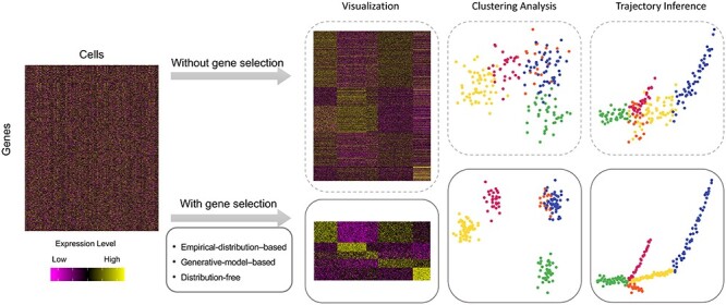
A diagram showing typical unsupervised analysis of single-cell gene expression data with or without gene feature selection. Clustering analysis is the task of grouping individual cells such that cells in the same cluster have more similar gene expression levels to each other than to those in other clusters. Trajectory analysis is the task of computationally inferring the pseudotime order of individual cells along developmental trajectories. In general, unsupervised analysis of single cells has increased accuracy when performed after gene feature selection. We refer readers to previous review articles [15, 20, 21] for a more complete workflow of scRNA-seq analysis starting from processing of raw data.
We summarize the importance of gene feature selection in scRNA-seq analysis in three aspects. First, in terms of biological interpretation, accurate identification of gene features can help reveal heterogeneous cell populations and unique gene expression patterns in specific cell types or cell states. In particular, isolating informative genes of rare cell populations is the key to detecting novel cell types [22]. Second, in terms of statistical modeling, gene selection can help overcome the so-called curse of dimensionality problem and explore cellular similarities in a lower dimensional space where cell–cell distances are more reliable. For example, two fundamental unsupervised learning tasks, clustering analysis and trajectory analysis [23, 24], both heavily rely on the ability to faithfully model cellular similarities given informative gene features [16] (Figure 1). Genes whose actual abundance does not vary among different cell types or cell states only contribute technical noises to the calculation of cellular similarities, compromising the accuracy of unsupervised analyses if not being excluded (Figure 1). Thus, a major goal of gene feature selection is to remove these non-relevant genes and retain those functionally important to the biological variability in the data. Third, in terms of computational efficiency, gene feature selection can significantly reduce the memory consumption and computational time of dimensionality reduction methods, especially nonlinear methods such as tSNE [25] and UMAP [26].
Even though feature selection has been routinely used as an intermediate step to solve diverse statistics and bioinformatics problems [27, 28], selecting gene features from single-cell gene expression data presents several unique challenges. First, read counts of the same gene in different cells are subject to cell-specific technical variability, so these counts cannot be treated as identical samples from the same underlying distribution. Thus, normalization needs to be either performed before the modeling step or incorporated into the statistical models [29, 30]. Second, single-cell gene expression data are highly sparse as a combined result of gene expression stochasticity, false negatives (the so-called ’dropouts’, indicating genes whose transcripts are expressed in a cell but undetected in its mRNA profile), and overamplification [2, 31, 32]. As a consequence, the gene selection methods need to account for the overdispersion of read counts resulted from the above factors. Third, scRNA-seq experiments are also subject to unexplained technical noises [33, 34], making it challenging to identify gene features that show genuine biological variability in their expression between different cell types or cell states.
In this article, we review the recent advances in gene selection methods for analyzing and modeling single-cell gene expression data. As gene selection is performed before cell labels are obtained in most cases, we focus on the context of unsupervised learning, where gene features are selected by evaluating the distribution and variance of gene expression levels. In summary, we divide the existing methods into three major categories: empirical-distribution–based, generative-model–based and distribution-free. The key characteristics of these methods are summarized in Table 1. For each category of methods, we first introduce the statistical assumptions and approaches that are shared by most methods, then discuss those that are unique to specific methods. In addition to the methods summarized in Table 1, there are single-cell studies that select genes purely based on known gene signatures [35]. There are also feature selection approaches embedded in computational methods for downstream analysis, such as clustering [36] and trajectory inference [37]. We do not include these two types of methods as they are less generalizable for future method development and have relatively limited applications in real practice.
Table 1.
Gene feature selection methods for unsupervised analysis of single-cell gene expression data
|
|

2 The feature selection problem in scRNA-seq data analysis
2.1 Notations
We first introduce a set of notations used throughout our discussion. After alignment, the summarized read (or UMI) counts in single cells are denoted as an  matrix
 |
(1) |
where  is the read count of gene
  in cell
  ,
,  is the number of genes, and
  is the number of cells. Given a count matrix
  , we introduce several commonly used statistics. The sample mean of gene
  is denoted as
 |
(2) |
and the sample variance is
 |
(3) |
The corresponding population mean and variance are denoted as  and
and  , respectively. In addition, gene
  ’s frequency of zero counts is calculated as
 |
(4) |
To be consistent with several methods that model the frequency of zero counts,  is also referred to as the observed dropout rate of gene
  . Depending on the models being used, some gene selection methods need to perform normalization and/or log transformation on the observed count matrix before the selection metrics can be calculated. With a slight abuse of notation, for each method we will describe whether counts are normalized and use
  to denote either the observed or normalized count matrix.
2.2 Empirical-distribution–based methods
Empirical-distribution–based methods directly calculate summary statistics of all genes based on the empirical distribution of gene expression across single cells, and then select gene features by ranking these summary statistics. Commonly used statistics include empirical gene expression variance or dispersion, so those genes with high ranks are often referred to as highly variable genes (HVGs). Empirical-distribution–based methods are computationally efficient and do not require any prior knowledge of genes involved in relevant biological processes, but they usually need an arbitrary threshold on the summary statistics or feature number to select genes from the ranked list. In this subsection, we summarize seven methods that implement empirical-distribution–based gene selection (Table 1A). Four of them are stand-alone gene selection methods and the other three perform gene selection as an intermediate step in scRNA-seq analysis. These seven methods are characteristic of empirical-distribution-based methods used in real practice.
2.2.1 DISP, MVP and VST
We first introduce three methods provided by the Seurat package [38, 39]. It is also worth noting that the Python toolkit SCANPY [40] reproduces the implementations of Seurat for gene selection. The first method is DISP (short for dispersion) and it is applied to the count matrix after library size normalization. The DISP method performs gene selection based on log transformed gene expression dispersion, which is defined as the variance-to-mean ratio  . Genes with larger expression dispersion are selected with higher priority. This method is connected to the Negative Binomial models that will be discussed in the next subsection, which use the dispersion parameter to account for possible overdispersion of read counts.
The second method is MVP (short for mean-variance plot), which tries to identify variable genes while controlling for the relationship between gene expression variability and expression mean. Its rationale is to pool genes with similar average expression into several subsets and then calculate expression variability within each subset. The MVP method is applied to the normalized count matrix. It divides genes into  equal-sized subsets based on their natural logarithmic average expression
  . MVP calculates a
  statistic of the gene expression dispersion for gene
  , using the mean expression and standard deviation of the subset that gene
  belongs to:
 |
(5) |
where  is the subset that gene
  belongs to. Genes are finally ranked based on the
  statistics.
The third method is VST (short for variance stabilizing transformation), which accounts for the variance-mean relationship of gene expression with a regression model. VST first computes the gene expression mean  and variance
  using the observed counts and then applies log
 transformation on both. Next, it uses a LOESS regression model [41] to fit the relationship between them, with logarithmic variance
  as the response and logarithmic mean
  as the predictor. We denote the estimated variance by the regression as
  for gene
  . Using the estimated variance, VST standardizes read counts without removing higher-than-expected variation. It calculates a
  statistic of gene
  in cell
  as
as
 |
(6) |
To reduce the impact of technical outliers, VST clips the  statistics to a maximum value of
  (
( is the cell number). Then, for each gene
  , it computes the variance of the
  statistics across all cells, which is denoted as
  . Finally, genes are ranked based on
  .
.
2.2.2 scran
Next, we introduce the gene selection method provided by the scran package [42]. scran first normalizes the observed counts by library size and then applies log transformation to the gene expression. It then selects HVGs with two major steps: (i) identifying HVGs, and (ii) identifying highly correlated gene pairs among the HVGs. In the first step, scran searches for HVGs while accounting for the variance-mean relationship of gene expression, which is achieved by fitting a polynomial or LOESS [41] curve between the gene expression variance and the expression mean across all genes. We denote the estimated variance as
  for gene
  . Then, scran defines the biological component of gene
  ’s expression variance as
  , which is used to rank and select HVGs. In the second step, scran tries to remove falsely identified HVGs caused by random noise. Among the candidate HVG set, the correlation between every gene pair is quantified by a modified version of Spearman’s correlation coefficient. The significance of the correlation coefficients is assessed with a permutation method, and significant HVG pairs are those with
  values
  after false discovery rate (FDR) correction. Then, only genes that are significantly correlated with at least one other gene are retained as the final HVGs, whereas other genes are excluded from downstream analysis.
2.2.3 scVEGs
The fifth method, scVEGs [43], identifies HVGs while accounting for the relationship between genes’ coefficient of variation and mean expression levels. scVEGs is applied to the count matrix after library size normalization. Inspired by the Negative Binomial distribution, scVEGs proposes an additive model for expression variation to decompose it into technical and biological components. It assumes the following relationship between the population expression variance and expression mean
 |
(7) |
where  denotes the dispersion parameter,
  denotes an additive technical noise component, and
  ,
,  . It follows that
 |
(8) |
where  is gene
  ’s coefficient of variation (CV). Then, scVEGs uses sample CVs (
 ) and sample means (
 ) to estimate
  and
and  by fitting a local regression model with the R package locfit [44]. Finally, scVEGs ranks genes based on the difference between the sample CVs and the fitted values from the regression model.
2.2.4 scGEAToolbox
The sixth method, scGEAToolbox [45], also controls for the variance-mean relationship of gene expression as scran and scVEGs do. scGEAToolbox considers three sample statistics of each gene: expression mean  , coefficient of variation
  , and dropout rate
  . After normalization, it fits a spline function based on piece-wise polynomials to model the relationship among the three statistics, and calculates the distance between each gene’s observed statistics to the fitted 3D spline surface. Genes with larger distances are ranked higher for feature selection.
2.2.5 SLICER
The seventh method that selects genes based on the empirical distribution of gene expression is SLICER [46]. It aims to select genes whose expression shows more gradual variation across neighboring cells than at a global scale. SLICER first calculates genes’ mean expression ( ) and variance (
 ) after performs normalization and log transformation. Then, it identifies
  nearest neighbors of each cell based on cell–cell distances of normalized gene expression levels. Given the
  -nearest neighbor graph, it computes the neighborhood variance of each gene
  as
as
 |
(9) |
where  is the index of the
  -th nearest neighbor of cell
  . Finally, SLICER selects all genes whose overall variance is greater than the neighborhood variance (
 ) as the retained features.
2.3 Generative-model–based methods
In this subsection, we introduce generative-model–based methods, which use generative statistical models to describe the joint probability distribution of read counts and subsequently select gene features based on estimated gene expression parameters (Table 1B). Unlike empirical-distribution–based methods, generative-model–based methods first set up models and assumptions for gene expression and read generation processes, and then derive parameter estimates that can be used to identify HVGs. Some methods also provide inference tools for testing the significance of HVGs, eliminating the need to arbitrarily set a threshold on estimated parameters for gene selection. Compared with empirical-distribution–based methods, generative-model–based methods are often computationally more intensive, but they have the following advantages. First, they are more flexible to account for various sources of cell-specific effects. Second, they are able to borrow information across cells and/or genes, leading to more robust estimates given sparse and noisy single-cell gene expression data. Third, they allow decomposition of gene expression variability into biological and technical components, enabling the selection of gene features based only on biological variability. Even though some empirical-distribution–based methods, including scran and scVEGS, also involve the concept of estimating biological variation, generative-model–based methods allow explicit and separate models for the gene expression process and read generation process during estimation.
An important factor for selecting a proper generative-model–based method is whether or not extrinsic spike-in control genes have been used in the scRNA-seq experiments. If included in the experiments, the spike-in transcripts are added to each cell’s lysate with theoretically constant and known concentration [47]. Therefore, we further divide generative-model–based methods into two subcategories, depending on whether the methods use the read counts of spike-ins in their models. Normally, methods that require spike-in information use the read counts of nonbiological spike-in genes to quantify the effect of technical noises such as molecular capture efficiency or other unexplained sources, and then use the estimated technical effect to decompose the variability of biological genes into technical and biological components. In contrast, methods that do not require spike-in information directly use overdispersed models to account for biological and technical variability of biological genes.
2.3.1 Methods requiring spike-in information
We first introduce two methods developed to select HVGs given the availability of synthetic spike-ins in scRNA-seq experiments (Table 1B.1). The first method was proposed by Brennecke et al. [33], and we refer to it as Brennecke for short; the second method is BASiCS [34]. We first discuss the common statistical framework shared by both methods, then discuss the additional assumptions and modeling steps that are unique to each method. When spike-in information is available, we assume there are totally  gene features, including
  biological genes and
  spike-in genes (or technical genes).
Both Brennecke and BASiCS work with summarized UMI counts, and they use the Poisson distribution to model the read counts of biological and spike-in genes. Their major statistical model can be summarized as:
 |
(10) |
where  and
and  denote the library-specific effects;
  and
and  represent the abundance of transcripts from a biological or spike-in gene in library
  , respectively. Since the abundance of spike-in genes is only subject to technical variability, but the abundance of biological genes is subject to both technical and biological variability, different assumptions are applied to
  and
and  . Both Brennecke and BASiCS use spike-ins to estimate the technical effects, which are then used to deconvolve the variability of biological genes into technical and biological components.
2.3.2 Brennecke
Based on model (10), Brennecke further assumes that the expected abundance of each spike-in’s transcripts is the same across libraries, and the variance of each spike-in’s abundance depends on its mean through a quadratic function:
 |
(11) |
where  is the expected abundance of spike-in
  in each library;
  and
and  are parameters to be estimated;
  is the library size normalization factor (as defined in the DESeq2 method [48]) calculated only using spike-in genes. For biological genes, in addition to the variability of
  (the transcript abundance of biological gene
  in library
  ), Brennecke also considers the variability of
  (the transcript abundance of biological gene
  in cell
  ). To summarize, Brennecke models biological genes by integrating the following assumptions with model (10):
 |
(12) |
where  is the squared coefficient of biological variation for gene
  ;
;  denotes the proportion of biological transcripts in cell
  extracted to library
  ;
;  is the library size normalization factor calculated only using biological genes;
  and
and  are estimated using spike-in genes. Note that a key assumption in this step is that conditional on a biological gene’s abundance in cell
  (
( ), the expectation of its abundance in library
  ,
,  , depends on the ratio of extracted biological transcripts to the amount of spike-in transcripts.
Given parameters estimated with the above model, Brennecke detects HVGs based on the relationship between the estimated gene expression mean ( ) and squared coefficient of variation (
 ) (
) ( ). It defines HVGs as genes whose expression variability substantially exceeds expected technical variability. This detection is achieved by a hypothesis test. The null hypothesis is
  , meaning that a gene’s biological CV
 does not significantly exceed a predetermined level
  . Under
  , it constructs a test statistic that approximately follows a
  distribution with
  degrees of freedom, from which the
  value can be derived.
2.3.3 BASiCS
The BASiCS method is also based on model (10), but is formulated under a Bayesian framework. For spike-in genes, it assumes that the unexplained technical noise (modeled with  ) depends on library-specific effects, and influences the abundance of all genes in a library in the same manner. Therefore, BASiCS models the spike-in genes’ abundance as follows:
 |
(13) |
where  is the transcript abundance of spike-in gene
  in each library;
  is the expected molecular capture efficiency of library
  ;
;  is a hyperparameter denoting the strength of unexplained technical noise. For biological genes, the key assumption in BASiCS is that the transcript abundance of biological gene
  in library
  is affected by the total cellular mRNA content, which is modeled through
  , and the heterogeneous expression of the gene across cells, which is modeled through
  . BASiCS models the biological genes’ abundance as follows:
 |
(14) |
where  is the normalized transcript abundance of biological gene
  in each cell;
  is a measure representing biological variability of gene expression across cells;
  is a gene-specific hyperparameter;
  is a cell-specific factor representing the total mRNA content in cell
  .
.
Given the above model, BASiCS decomposes the variance of each biological gene’s read count,  , into three components: the variance introduced by the biological cell-to-cell heterogeneity (
 ), the sequencing process (
 , based on the Poisson model) and the unexplained technical sources (
 ). Therefore, HVGs can be selected by comparing
  , the proportion of read counts’ variation that is explained by biological cell-to-cell heterogeneity in a typical cell:
 |
(15) |
BASiCS quantifies the evidence of a gene being highly variable using the upper tail posterior probabilities of  . Given a threshold
  on the proportion of biological variation and an evidence threshold
  , it selects HVGs such that
 |
(16) |
2.3.4 Methods not requiring spike-in information
In this subsection, we introduce five generative-model–based methods that only need the count matrix of biological genes to select gene features (Table 1B.2). Three of these methods have the same basic assumption that the read count of each gene in each cell follows a Negative Binomial (NB) distribution:
 |
(17) |
where  is the unknown true abundance of gene
  in cell
  , and
, and  is the dispersion of gene
  ’s expression. Therefore, the variance of gene
  in cell
  is
is  .
.
2.3.5 sctransform
We first introduce sctransform [49], which was developed to model UMI counts based on the assumption of NB distribution. The first step of sctransform is to fit a generalized linear model (GLM) for each gene by integrating model (17) with the following assumption:
 |
(18) |
where  is the total number of UMI counts in cell
  . This step aims to correct for different sequencing depths among the cells. After fitting the GLM, we denote the estimated parameters as
  and
and  . The second step of sctransform is to address the overfitting issue caused by unconstrained NB models used in the first step. To share information across genes, it constructs a separate kernel regression model to fit the global trend between each of the three parameters (
 and
and  ) and gene expression mean. The regularized parameter estimates, denoted as
  and
and  , are the fitted values from the regression models. These regularized parameters are then used to standardize the counts in the third step. In this step, sctransform standardizes the UMI counts to obtain Pearson residuals:
 |
(19) |
where  , and
, and  . In particular, a positive residual of a gene in a cell suggests that more UMIs are observed than expected, after accounting for the gene’s mean expression and sequencing depths. To reduce the impact of outlier counts, sctransform then clips the absolute Pearson residuals to a maximum value of
  . In order to select HVGs, sctransform ranks genes by the variance of their Pearson residuals.
It is worth mentioning that sctransform can be viewed as a model-based extension of the VST method. In VST, the estimation of gene expression mean and regularized variance is based on sample mean and variance, whereas in sctransform, the estimation is based on an NB model to account for sequencing depth.
2.3.6 NBDisp and NBDrop
The second and third methods, NBDisp and NBDrop [50], are also based on the assumption of NB distribution. For gene  , they first estimate the mean and dispersion parameters in the NB model, which we denote as
  and
and  . Next, NBDisp selects gene features based on expression dispersion whereas NBDrop is based on dropout rate. NBDisp fits a linear regression model between the estimated dispersion and log transformed mean expression across all genes
 |
(20) |
It then uses residuals from this regression model to rank genes and select those with highly dispersed expression. In contrast, NBDrop calculates the expected dropout rate of gene  as
as
 |
(21) |
and then obtains  values of observed dropout rates (
 ) based on a Binomial model.
2.3.7 HIPPO
The fourth method, HIPPO [24], leverages zero proportions in the count data to detect cellular heterogeneity and identify gene features. In contrast to the above three methods that assume an NB distribution, which is a compound Poisson-Gamma distribution, HIPPO uses a finite mixture of Poisson distribution to model the UMI counts. It considers the gene selection problem in the context of hypothesis testing. For each gene, the null hypothesis assumes that its expression is not subject to biological variability, and its counts follow a Poisson distribution:  , where
  is the mean parameter (
 ). The alternative hypothesis assumes that its expression presents biological variability, and the counts follow a mixture Poisson distribution:
  , where
  indicates the number of cell subpopulations,
  and
and  are the proportion and mean parameter for the corresponding subpopulation, respectively. To test the hypotheses, HIPPO evaluates if the observed dropout rate of a gene,
  , is significantly larger than the expected proportion under the null hypothesis,
  . The test statistic is a
  statistic, and genes can be selected by ranking the
  statistics or setting a threshold on their corresponding
  values. In addition to this criterion, HIPPO also allows the selection of genes based on a deviance statistic derived from the Poisson model.
2.3.8 Townes
The fifth method uses the Multinomial distribution to model the UMI counts [51]. We refer to the method as Townes for short. Townes assumes that the UMI counts in each cell follow a multinomial distribution,
 |
(22) |
where  is the total UMI count in the cell
  , and
, and  is the unknown true relative abundance of gene
  in cell
  . Ignoring the correlation between the genes (as
  ’s are small), Townes further approximates the count distribution of gene
  in cell
  with a Binomial distribution:
  . Like HIPPO, Townes also selects HVGs in the context of hypothesis testing. The null hypothesis is that a gene’s true relative abundance is constant across cells:
  . A deviance statistic can be derived based on the Binomial model under the null hypothesis to assess the goodness of fit. Although Townes et al. suggested to directly select genes by ranking them according to their deviances, it is also possible to obtain
  values of the genes using the Binomial deviance.
2.4 Distribution-free methods
In addition to empirical-distribution–based methods and generative-model–based methods for gene feature selection, there are also methods adapted from other commonly used variability measures to identify gene features. These methods often do not assume a specific statistical model, and instead directly calculate a dispersion measure to quantify the variability of gene expression in single cells. We focus on three methods, among which EDGE [52] uses the entropy measure in information theory, GiniClust [53] uses Gini index from economics, and M3Drop [50] derives a measure based on the Michaelis–Menten kinetics model [54].
2.4.1 EDGE
EDGE [52] is an ensemble method for simultaneous dimensionality reduction and feature gene extraction. Here we only discuss its feature gene selection procedure. EDGE first normalizes the count matrix by library sizes and then applies the  transformation. Then, the gene selection procedure takes
  sets of single cell partitions as the input. Each partition is a grouping of all cells into nonempty and nonoverlapping subsets, and is independently learned by randomly selecting
  genes as the features and comparing cellular similarities based on the normalized expression of the selected
  genes. Based on each partition, a binary similarity matrix is constructed with 1 indicating that the corresponding two cells are assigned to the same cluster. A clustering algorithm based on a nearest neighbor graph is then applied to the average similarity matrix across the
  partitions. We use
  to denote the number of obtained cell clusters. Next, for the
  -th partition, the entropy of its selected
  genes is calculated as
 |
(23) |
where  is the number of cell groups in partition
  , and
, and  is the proportion of the
  -th cell cluster in the
  -th cell group. It then calculates the entropy of each gene
  as
as
 |
(24) |
Let  and
and  be the mean and standard deviation of
  . EDGE uses
  as the cut-off value on the entropy scores to select top gene features. In addition to EDGE, there are also discussions of using information theory measures to select gene markers in the context of supervised learning, when cell labels are known [55].
2.4.2 GiniClust
GiniClust [53] was designed to identify rare cell types using single-cell gene expression data, and it includes a gene selection procedure based on the Gini index [56]. Its developers have found that the Gini index could effectively identify rare cell-type-specific genes. The procedure consists of three steps. In the first step, the Gini index is calculated using normalized gene expression levels. For each gene  , GiniClust ranks the single cells based on the gene’s expression level from the lowest to the highest. A Lorenz curve [56] is then obtained to represent the relationship between the gene’s accumulated expression levels and cell proportions. The
  -axis of the curve denotes the proportion of cells taken from the top of the ranked list, and the
  -axis denotes the ratio between the summed gene expression levels in these cells and the summed gene expression levels in all cells. Next, the Gini index,
  , is defined as two times the area between the Lorenz curve and the diagonal curve (
 ). In the second step, GiniClust normalizes the Gini indices calculated in the first step to remove the correlation trend between the Gini index and the genes’ maximum gene expression levels. This is achieved by a LOESS regression model, and the normalized Gini index
  is calculated as the residual from the LOESS regression. Finally, GiniClust selects gene features by ranking the normalized Gini index or by thresholding tail probabilities estimated with a Gaussian approximation.
2.4.3 M3Drop
Lastly, we introduce M3Drop [50], which performs gene feature selection based on the Michaelis–Menten kinetics model, after normalizing the read counts. M3Drop assumes that dropout events are due to failure of the reverse transcription, a simple enzyme reaction, and thus should be modeled using the Michaelis–Menten equation,
 |
(25) |
where  is a parameter representing the expected expression level of gene
  when the dropout rate is 50%, and
  is the observed dropout rate of gene
  . It follows that
  . In addition, M3Drop estimates a global parameter
  by fitting
  across all genes, and we denote the estimate as
  . For gene
  , M3Drop determines if the gene-specific parameter significantly differs from the global parameter using the tail probabilities of
  calculated based on a log-normal approximation.
3 Comparing gene feature selection methods used in real practice
3.1 A summary of gene selection methods used in real practice
To find out the choices of gene selection methods in real practice, we surveyed 415 studies published in 2020 or the first quarter of 2021, based on a curated database of published single-cell transcriptomics data [57]. Among these studies, 314 described the gene selection methods used before unsupervised downstream analyses such as clustering or trajectory analysis (Figure S1A). We found that Seurat is currently the most commonly used package, with more than half of the studies using it (DISP, VST, or MVP) for feature selection. The second most popular tool is sctransform, which has also been implemented in the Seurat package. Another frequently used tool is SCANPY [40], which is a Python-based toolkit for analyzing single-cell gene expression data. We have also noticed studies that proposed their own statistics for selecting HVGs [58, 59]. Like many methods discussed in this article, they define a dispersion statistic after accounting for the mean-variance relationship in single-cell gene expression data.
We also summarized the number of gene features selected in the above studies (Figure S1B). Overall, 153 studies have reported the number of selected genes. The minimum number of used gene features was 242 [60], and the maximum was 16 471 [61]. More than 65% studies chose 1000–3000 gene features, and this is possibly because the default number set in most software is within this range. In cases where multiple single-cell gene expression datasets were analyzed in the same study, researchers often selected 1000–2000 feature genes in each dataset, and then either took the union or the intersection of these genes as the selected gene features [62, 63].
3.2 Comparing gene feature selection methods with a case study
According to the above summary, most recent studies chose to use software toolkits (such as Seurat and SCANPY) to perform gene feature selection with default parameters in the software. To investigate how the choices of gene selection methods and selection criteria affect scRNA-seq analysis, we performed a case study by evaluating the downstream clustering accuracy. We used a scRNA-seq dataset (with UMI counts) from an R package DuoClustering2018 [64, 65]. We chose this dataset because the cell populations have been sorted by the flow cytometry technology, providing ground truth information of true cell clusters. The original dataset contains 3994 cells and 15 716 gene features. The cells were grouped into eight cell types: B cells, naive cytotoxic T cells, CD14 monocytes, regulatory T cells, CD56 NK cells, memory T cells, CD4 T-helper cells, and naive T cells.
To evaluate the gene selection performance with data of different sparsity levels, we considered three datasets in our analysis: (i) the original count matrix (Dataset 1); (ii) subsetted count matrix using 50% cells with the largest gene detection rate from each cell type (Dataset 2); (iii) subsetted count matrix using 50% cells with the lowest gene detection rate from each cell type (Dataset 3). We included thirteen gene selection methods that are directly applicable to the above UMI datasets in our analysis. In addition to selecting genes based on software’s default parameters, for nine methods that can output calculated gene-wise statistics, we also tried to select different numbers of gene features (500, 1000, and 2000) to better compare their performance in different scenarios (see details in the Supplementary Methods). For each dataset and gene selection method, we first selected gene features, then applied Seurat to perform clustering just using the selected genes. The clustering accuracy was evaluated using the adjusted Rand index (ARI) (Supplementary Methods).
Comparing the thirteen gene selection tools with their corresponding default parameters (Figure 2), we found that scGEAToolbox and HIPPO had the best performance on data with relatively low sparsity, whereas NBDisp and Towns were the best on data with relatively high sparsity. Comparing the same method’s performance with different number of selected genes, we found that some methods, including sctransform, NBDisp, scGEAToolbox, and GiniClust, were more sensitive to the number of selected features, whereas Townes and NBDrop were more robust (Figure 2). In addition, for NBDrop, scran, DISP, and GiniClust, the default parameters did not always lead to the highest clustering accuracy. Overall, generative-model–based methods tended to have more advantageous performance when data were sparser. Lastly, we also compared the computational time of these gene selection tools, and all methods, except for SLICER and scran, were able to finish the computation within 100 seconds (Figure S2).
Figure 2 .

A comparison of clustering accuracy based on gene features selected by different methods. The methods were compared based on their performance on Dataset 1 (A, the original dataset), Dataset 2 (B, relative low sparsity level) and Dataset 3 (C, relative high sparsity level). For each dataset and gene selection method, the clustering accuracy was measured by ARI using genes selected with default parameters or the top 500/1000/2000 genes ranked by the corresponding selection criteria. Please note that only nine software tools allow users to select an arbitrary number of genes based on their output.
4 Discussion
In this article, we summarize and discuss 17 computational methods for selecting gene features in unsupervised analysis of single-cell gene expression data, with unified notations and statistical frameworks. These methods include seven empirical-distribution–based methods, seven generative-model–based methods, and three distribution-free methods that depend on popular uncertainty measures such as the Shannon entropy and Gini index. Unlike empirical-distribution–based methods that do not depend on distributional assumptions, generative-model–based methods directly use count models to account for biological and technical sources of variability, so they do not need special normalization and data transformation before the modeling step. Even though the two categories of methods use different statistical frameworks, most methods account for the relationship between gene expression variance and expression mean to select truly informative gene features. Otherwise, genes with high mean expression levels would have a greater chance of being selected than those with low expression levels.
Our review provides the most comprehensive summary of currently available gene selection methods in scRNA-seq analysis. It is complementary to existing reviews that focused on a few methods and computational performance in clustering analysis [18, 19]. We focus on gene selection methods that have been implemented as software packages or stand-alone functions. There are also additional gene selection methods embedded in tools for unsupervised analysis of single-cell gene expression data [58, 66]. For example, STREAM [67] internally implements empirical-distribution–based gene feature selection to reconstruct single-cell trajectories. RaceID3 [68] also uses an empirical-distribution–based gene selection method before performing clustering analysis.
Our survey of recently published scRNA-seq studies shows that the majority of these studies used software toolkits for scRNA-seq analysis, such as Seurat and SCANPY, to perform gene feature selection. However, it is yet unclear which selection method would lead to the optimal performance for different downstream analyzing tasks. In addition, evaluation of whether and how the number of retained gene features influences downstream analysis is also in need to optimize the current practice for feature selection. Our case study, based on one real dataset of peripheral blood mononuclear cells and the clustering method in Seurat, demonstrates that the generative-model–based methods tend to outperform the others when data is relatively sparse. Our analysis also shows that it would be helpful to output calculated selection statistics in addition to an arbitrary list of selected genes, allowing users to adjust the number of selected gene features when the default settings do not lead to a satisfying performance. When additional data with ground truth cell type labels and spike-ins become available, it would be interesting to investigate if the same conclusions hold for other datasets and clustering methods. As multiple simulation tools have become available to generate synthetic single-cell gene expression data under various experimental settings [69–71], we anticipate that these gene selection methods can be comprehensively benchmarked across sequencing platforms and for various downstream analyzing tasks.
In addition to scRNA-seq technologies for profiling single-cell transcriptomes, other methods have also emerged to profile DNA modifications, DNA accessibility, chromosome organization and proteomes in single cells [72]. As the identification of cell identities or cell states is a key step in unsupervised analysis of single cells, the gene selection methods developed for scRNA-seq data could be modified and extended to identify highly variable proteins or variable peaks resulted from epigenome profiling [73, 74]. Meanwhile, as spatially resolved transcriptomic methods have become available [75], the additional layer of spatial localization information leads to a new computational problem. That is, to identify spatially variable genes that have expression patterns associated with spatial coordinates [76, 77]. In summary, we expect this article to provide a useful summary to practitioners in the field about the applicability and key assumptions of major gene selection methods. It also summarizes the statistical frameworks used in single-cell gene selection for method developers.
Key Points
Gene feature selection is a key step in unsupervised analysis of single-cell gene expression data in order to identify functionally important genes, reduce dimensionality, and improve computational efficiency.
According to the statistical frameworks, gene selection methods for scRNA-seq analysis can be classified as empirical-distribution–based methods, generative-model–based methods, and distribution-free methods that depend on popular variability measures such as Shannon entropy and Gini index. These methods vary in terms of their applicability, distributional assumptions, and gene selection criteria.
Unlike empirical-distribution–based methods that do not depend on distributional assumptions, generative-model–based methods directly use count models to account for biological and technical sources of variability. Even though the two categories of methods use different statistical frameworks, most methods account for the relationship between gene expression variance and expression mean to select truly informative gene features.
Generative-model–based methods often provide inference tools to select gene features based on a user-selected threshold on the statistical significance, whereas the other methods require a threshold on a variance or dispersion measure to select gene features.
Supplementary Material
Acknowledgments
The authors thank the anonymous reviewers for their valuable suggestions.
Jie Sheng is a graduate student at University of Wisconsin - Madison with a background in mathematics, statistics, and data science. Her research interest lies in theoretical and computational statistics, machine learning, bioinformatics and computational biology.
Wei Vivian Li is an assistant professor at the Department of Biostatistics and Epidemiology of Rutgers, The State University of New Jersey. She has a Ph.D. degree in Statistics and her research focuses on statistical and machine learning methods for genomic and other biological data.
Contributor Information
Jie Sheng, Department of Statistics, University of Wisconsin-Madison, Madison, WI 53706, USA.
Wei Vivian Li, Department of Biostatistics and Epidemiology, Rutgers School of Public Health, Piscataway, NJ 08854, USA.
Data availability
The source code used to replicate our analysis is available at this link: https://github.com/JieShengm/Feature_Gene_Selection.
Funding
National Institutes of Health (NIH) R21MH126420, NJ ACTS BERD Mini-methods Grant (a component of the NIH under Award Number UL1TR0030117), Rutgers Busch Biomedical Grant, and Rutgers School of Public Health Pilot Grant (to W.V.L.).
References
- 1. Kolodziejczyk AA, Kim JK, Svensson V, et al. The technology and biology of single-cell RNA sequencing. Mol Cell 2015;58(4):610–20. [DOI] [PubMed] [Google Scholar]
- 2. Wagner A, Regev A, Yosef N. Revealing the vectors of cellular identity with single-cell genomics. Nat Biotechnol 2016;34(11):1145–60. [DOI] [PMC free article] [PubMed] [Google Scholar]
- 3. Li WV, Li JJ. Modeling and analysis of RNA-seq data: a review from a statistical perspective. Quant Biol 2018;6(3):195–209. [DOI] [PMC free article] [PubMed] [Google Scholar]
- 4. Pisco AO, Schaum N, McGeever A, et al. A single cell transcriptomic atlas characterizes aging tissues in the mouse. Nature 2020;583(7817):590. [DOI] [PMC free article] [PubMed] [Google Scholar]
- 5. Travaglini KJ, Nabhan AN, Penland L, et al. A molecular cell atlas of the human lung from single-cell RNA sequencing. Nature 2020;587(7835):619–25. [DOI] [PMC free article] [PubMed] [Google Scholar]
- 6. Aizarani N, Saviano A, Sagar, et al. A human liver cell atlas reveals heterogeneity and epithelial progenitors. Nature 2019;572(7768):199–204. [DOI] [PMC free article] [PubMed] [Google Scholar]
- 7. Han X, Zhou Z, Fei L, et al. Construction of a human cell landscape at single-cell level. Nature 2020;581(7808):303–9. [DOI] [PubMed] [Google Scholar]
- 8. Regev A, Teichmann SA, Lander ES, et al. Science forum: the human cell atlas. Elife 2017;6:e27041. [DOI] [PMC free article] [PubMed] [Google Scholar]
- 9. Kumar MP, Du J, Lagoudas G, et al. Analysis of single-cell RNA-seq identifies cell-cell communication associated with tumor characteristics. Cell Rep 2018;25(6):1458–68. [DOI] [PMC free article] [PubMed] [Google Scholar]
- 10. Biddy BA, Kong W, Kamimoto K, et al. Single-cell mapping of lineage and identity in direct reprogramming. Nature 2018;564(7735):219–24. [DOI] [PMC free article] [PubMed] [Google Scholar]
- 11. Potter SS. Single-cell RNA sequencing for the study of development, physiology and disease. Nat Rev Nephrol 2018;14(8):479–92. [DOI] [PMC free article] [PubMed] [Google Scholar]
- 12. Papalexi E, Satija R. Single-cell RNA sequencing to explore immune cell heterogeneity. Nat Rev Immunol 2018;18(1):35. [DOI] [PubMed] [Google Scholar]
- 13. Lähnemann D, Köster J, Szczurek E, et al. Eleven grand challenges in single-cell data science. Genome Biol 2020;21(1):1–35. [DOI] [PMC free article] [PubMed] [Google Scholar]
- 14. Kivioja T, Vähärautio A, Karlsson K, et al. Counting absolute numbers of molecules using unique molecular identifiers. Nat Methods 2012;9(1):72–4. [DOI] [PubMed] [Google Scholar]
- 15. Hie B, Peters J, Nyquist SK, et al. Computational methods for single-cell RNA sequencing. Annu Rev Biomed Data Sci 2020;3:339–64. [Google Scholar]
- 16. Kiselev VY, Andrews TS, Hemberg M. Challenges in unsupervised clustering of single-cell RNA-seq data. Nat Rev Genet 2019;20(5):273–82. [DOI] [PubMed] [Google Scholar]
- 17. Hwang B, Lee JH, Bang D. Single-cell RNA sequencing technologies and bioinformatics pipelines. Exp Mol Med 2018;50(8):1–14. [DOI] [PMC free article] [PubMed] [Google Scholar]
- 18. Su K, Yu T, Wu H. Accurate feature selection improves single-cell RNA-seq cell clustering. Brief Bioinform 02 2021. bbab034. [DOI] [PMC free article] [PubMed] [Google Scholar]
- 19. Yip SH, Sham PC, Wang J. Evaluation of tools for highly variable gene discovery from single-cell RNA-seq data. Brief Bioinform 2019;20(4):1583–9. [DOI] [PMC free article] [PubMed] [Google Scholar]
- 20. Luecken MD, Theis FJ. Current best practices in single-cell RNA-seq analysis: a tutorial. Mol Syst Biol 2019;15(6):e8746. [DOI] [PMC free article] [PubMed] [Google Scholar]
- 21. Amezquita RA, Lun ATL, Becht E, et al. Orchestrating single-cell analysis with bioconductor. Nat Methods 2020;17(2):137–45. [DOI] [PMC free article] [PubMed] [Google Scholar]
- 22. Grün D, Lyubimova A, Kester L, et al. Single-cell messenger RNA sequencing reveals rare intestinal cell types. Nature 2015;525(7568):251–5. [DOI] [PubMed] [Google Scholar]
- 23. Germain P-L, Sonrel A, Robinson MD. pipeComp, a general framework for the evaluation of computational pipelines, reveals performant single cell RNA-seq preprocessing tools. Genome Biol 2020;21(1):1–28. [DOI] [PMC free article] [PubMed] [Google Scholar]
- 24. Kim TH, Zhou X, Chen M. Demystifying “drop-outs” in single-cell UMI data. Genome Biol 2020;21(1):1–19. [DOI] [PMC free article] [PubMed] [Google Scholar]
- 25. Van Maaten L, Hinton G. Visualizing data using t-SNE. J Mach Learn Res 2008;9(11):2579–605. [Google Scholar]
- 26. McInnes L, Healy J, Melville J. Umap: Uniform manifold approximation and projection for dimension reduction. arXiv preprint arXiv:1802.03426. 2018.
- 27. Ang JC, Mirzal A, Haron H, et al. Supervised, unsupervised, and semi-supervised feature selection: a review on gene selection. IEEE/ACM Trans Comput Biol Bioinform 2015;13(5):971–89. [DOI] [PubMed] [Google Scholar]
- 28. Hira ZM, Gillies DF. A review of feature selection and feature extraction methods applied on microarray data. Adv Bioinform 2015;2015:198363. [DOI] [PMC free article] [PubMed] [Google Scholar]
- 29. McCarthy DJ, Campbell KR, Lun ATL, et al. Scater: pre-processing, quality control, normalization and visualization of single-cell RNA-seq data in R. Bioinformatics 2017;33(8):1179–86. [DOI] [PMC free article] [PubMed] [Google Scholar]
- 30. Cole MB, Risso D, Wagner A, et al. Performance assessment and selection of normalization procedures for single-cell RNA-Seq. Cell Systems 2019;8(4):315–28. [DOI] [PMC free article] [PubMed] [Google Scholar]
- 31. Li WV, Li JJ. An accurate and robust imputation method scImpute for single-cell RNA-seq data. Nat Commun 2018;9(1):1–9. [DOI] [PMC free article] [PubMed] [Google Scholar]
- 32. Cao Z, Grima R. Analytical distributions for detailed models of stochastic gene expression in eukaryotic cells. Proc Natl Acad Sci 2020;117(9):4682–92. [DOI] [PMC free article] [PubMed] [Google Scholar]
- 33. Brennecke P, Anders S, Kim JK, et al. Accounting for technical noise in single-cell RNA-seq experiments. Nat Methods 2013;10(11):1093. [DOI] [PubMed] [Google Scholar]
- 34. Vallejos CA, Marioni JC, Richardson S. BASiCS: Bayesian analysis of single-cell sequencing data. PLoS Comput Biol 2015;11(6):e1004333. [DOI] [PMC free article] [PubMed] [Google Scholar]
- 35. Abdelaal T, Michielsen L, Cats D, et al. A comparison of automatic cell identification methods for single-cell RNA sequencing data. Genome Biol 2019;20(1):1–19. [DOI] [PMC free article] [PubMed] [Google Scholar]
- 36. Grün D. Revealing dynamics of gene expression variability in cell state space. Nat Methods 2020;17(1):45–9. [DOI] [PMC free article] [PubMed] [Google Scholar]
- 37. Qiu X, Mao Q, Tang Y, et al. Reversed graph embedding resolves complex single-cell trajectories. Nat Methods 2017;14(10):979. [DOI] [PMC free article] [PubMed] [Google Scholar]
- 38. Satija R, Farrell JA, Gennert D, et al. Spatial reconstruction of single-cell gene expression data. Nat Biotechnol 2015;33(5):495–502. [DOI] [PMC free article] [PubMed] [Google Scholar]
- 39. Stuart T, Butler A, Hoffman P, et al. William M Mauck III, Yuhan Hao, Marlon Stoeckius, Peter Smibert, and Rahul Satija. Comprehensive integration of single-cell data. Cell 2019;177(7):1888–902. [DOI] [PMC free article] [PubMed] [Google Scholar]
- 40. Wolf FA, Angerer P, Theis FJ. SCANPY: large-scale single-cell gene expression data analysis. Genome Biol 2018;19(1):1–5. [DOI] [PMC free article] [PubMed] [Google Scholar]
- 41. Cleveland WS. Robust locally weighted regression and smoothing scatterplots. J Am Stat Assoc 1979;74(368):829–36. [Google Scholar]
- 42. Lun ATL, McCarthy DJ, Marioni JC. A step-by-step workflow for low-level analysis of single-cell RNA-seq data with Bioconductor. F1000Research 2016;5, 2122. [DOI] [PMC free article] [PubMed] [Google Scholar]
- 43. Chen H-IH, Jin Y, Huang Y, et al. Detection of high variability in gene expression from single-cell RNA-seq profiling. BMC Genom 2016;17(7):119–28. [DOI] [PMC free article] [PubMed] [Google Scholar]
- 44. Catherine Loader . locfit: Local Regression, Likelihood and Density Estimation, 2020. R package version, 1.5–9.4.
- 45. Cai JJ. scGEAToolbox: a Matlab toolbox for single-cell RNA sequencing data analysis. Bioinformatics 2019;36(6):1948–49. [DOI] [PubMed] [Google Scholar]
- 46. Welch JD, Hartemink AJ, Prins JF. SLICER: inferring branched, nonlinear cellular trajectories from single cell RNA-seq data. Genome Biol 2016;17(1):1–15. [DOI] [PMC free article] [PubMed] [Google Scholar]
- 47. Vallejos CA, Risso D, Scialdone A, et al. Normalizing single-cell RNA sequencing data: challenges and opportunities. Nat Methods 2017;14(6):565. [DOI] [PMC free article] [PubMed] [Google Scholar]
- 48. Love MI, Huber W, Anders S. Moderated estimation of fold change and dispersion for RNA-seq data with DESeq2. Genome Biol 2014;15(12):1–21. [DOI] [PMC free article] [PubMed] [Google Scholar]
- 49. Hafemeister C, Satija R. Normalization and variance stabilization of single-cell RNA-seq data using regularized negative binomial regression. Genome Biol 2019;20(1):1–15. [DOI] [PMC free article] [PubMed] [Google Scholar]
- 50. Andrews TS, Hemberg M. M3Drop: dropout-based feature selection for scRNASeq. Bioinformatics 2019;35(16):2865–7. [DOI] [PMC free article] [PubMed] [Google Scholar]
- 51. Townes FW, Hicks SC, Aryee MJ, et al. Feature selection and dimension reduction for single-cell RNA-Seq based on a multinomial model. Genome Biol 2019;20(1):1–16. [DOI] [PMC free article] [PubMed] [Google Scholar]
- 52. Sun X, Liu Y, An L. Ensemble dimensionality reduction and feature gene extraction for single-cell RNA-seq data. Nat Commun 2020;11(1):1–9. [DOI] [PMC free article] [PubMed] [Google Scholar]
- 53. Jiang L, Chen H, Pinello L, et al. GiniClust: detecting rare cell types from single-cell gene expression data with Gini index. Genome Biol 2016;17(1):1–13. [DOI] [PMC free article] [PubMed] [Google Scholar]
- 54. Cornish-Bowden A. One hundred years of Michaelis–Menten kinetics. Perspect Sci 2015;4:3–9. [Google Scholar]
- 55. Varma U, Colacino J, Gilbert A. Information theoretic feature selection methods for single cell RNA-sequencing. bioRxiv. 2019;646919.
- 56. Gastwirth JL. The estimation of the Lorenz curve and Gini index. Rev Econ Stat 1972;54(3):306–16. [Google Scholar]
- 57. Svensson V, Veiga Beltrame E, Pachter L. A curated database reveals trends in single-cell transcriptomics. Database 2020;2020:baaa073. [DOI] [PMC free article] [PubMed] [Google Scholar]
- 58. Cowan CS, Renner M, de Gennaro M, et al. Cell types of the human retina and its organoids at single-cell resolution. Cell 2020;182(6):1623–40. [DOI] [PMC free article] [PubMed] [Google Scholar]
- 59. Sawada T, Chater TE, Sasagawa Y, et al. Developmental excitation-inhibition imbalance underlying psychoses revealed by single-cell analyses of discordant twins-derived cerebral organoids. Mol Psychiatry 2020;25(11):2695–711. [DOI] [PMC free article] [PubMed] [Google Scholar]
- 60. Zhang M, Eichhorn SW, Zingg B, et al. Molecular, spatial and projection diversity of neurons in primary motor cortex revealed by in situ single-cell transcriptomics. bioRxiv. 2020; doi: 10.1101/2020.06.04.105700. [DOI]
- 61. Jinling L, Yu Z, Chen Y, et al. Single-cell RNA sequencing of human kidney. Scientific Data 2020;7(1):4. [DOI] [PMC free article] [PubMed] [Google Scholar]
- 62. Kirita Y, Haojia W, Uchimura K, et al. Cell profiling of mouse acute kidney injury reveals conserved cellular responses to injury. Proc Natl Acad Sci 2020;117(27):15874–83. [DOI] [PMC free article] [PubMed] [Google Scholar]
- 63. Nathan A, Beynor JI, Baglaenko Y, et al. Multimodal memory T cell profiling identifies a reduction in a polyfunctional Th17 state associated with tuberculosis progression. bioRxiv. 2020; doi: 10.1101/2020.04.23.057828. [DOI]
- 64. Duó A, Soneson C. DuoClustering2018: Data, Clustering Results and Visualization Functions From Duó et al (2018), 2020, R package version 1.8.0https://bioconductor.org/packages/release/data/experiment/html/DuoClustering2018.html.
- 65. Zheng GXY, Terry JM, Belgrader P, et al. Massively parallel digital transcriptional profiling of single cells. Nat Commun 2017;8(1):1–12. [DOI] [PMC free article] [PubMed] [Google Scholar]
- 66. Pandey S, Shekhar K, Regev A, et al. Comprehensive identification and spatial mapping of habenular neuronal types using single-cell RNA-seq. Curr Biol 2018;28(7):1052–65. [DOI] [PMC free article] [PubMed] [Google Scholar]
- 67. Chen H, Albergante L, Hsu JY, et al. Single-cell trajectories reconstruction, exploration and mapping of omics data with STREAM. Nat Commun 2019;10(1):1–14. [DOI] [PMC free article] [PubMed] [Google Scholar]
- 68. Herman JS, Sagar, Grün D. FateID infers cell fate bias in multipotent progenitors from single-cell RNA-seq data. Nat Methods 2018;15(5):379. [DOI] [PubMed] [Google Scholar]
- 69. Li WV, Li JJ. A statistical simulator scDesign for rational scRNA-seq experimental design. Bioinformatics 2019; 35(14): i41–50. [DOI] [PMC free article] [PubMed] [Google Scholar]
- 70. Sun T, Song D, Li WV, et al. scDesign2: an interpretable simulator that generates high-fidelity single-cell gene expression count data with gene correlations captured. Genome Biol 2021;22:163. 10.1186/s13059-021-02367-2. [DOI] [PMC free article] [PubMed] [Google Scholar]
- 71. Zappia L, Phipson B, Oshlack A. Splatter: simulation of single-cell RNA sequencing data. Genome Biol 2017;18(1):1–15. [DOI] [PMC free article] [PubMed] [Google Scholar]
- 72. Kelsey G, Stegle O, Reik W. Single-cell epigenomics: Recording the past and predicting the future. Science 2017;358(6359):69–75. [DOI] [PubMed] [Google Scholar]
- 73. Ranjan B, Sun W, Park J, et al. DUBStepR: correlation-based feature selection for clustering single-cell RNA sequencing data. bioRxiv. 2020. doi: 10.1101/2020.10.07.330563 . [DOI]
- 74. Chen H, Lareau C, Andreani T, et al. Assessment of computational methods for the analysis of single-cell ATAC-seq data. Genome Biol 2019;20(1):1–25. [DOI] [PMC free article] [PubMed] [Google Scholar]
- 75. Marx V. Method of the Year: spatially resolved transcriptomics. Nat Methods 2021;18(1):9–14. [DOI] [PubMed] [Google Scholar]
- 76. Sun S, Zhu J, Zhou X. Statistical analysis of spatial expression patterns for spatially resolved transcriptomic studies. Nat Methods 2020;17(2):193–200. [DOI] [PMC free article] [PubMed] [Google Scholar]
- 77. Svensson V, Teichmann SA, Stegle O. SpatialDE: identification of spatially variable genes. Nat Methods 2018;15(5):343–6. [DOI] [PMC free article] [PubMed] [Google Scholar]
Associated Data
This section collects any data citations, data availability statements, or supplementary materials included in this article.
Supplementary Materials
Data Availability Statement
The source code used to replicate our analysis is available at this link: https://github.com/JieShengm/Feature_Gene_Selection.