bayesynergy: flexible Bayesian modelling of synergistic interaction effects in in vitro drug combination experiments

Abstract

The effect of cancer therapies is often tested pre-clinically via in vitro experiments, where the post-treatment viability of the cancer cell population is measured through assays estimating the number of viable cells. In this way, large libraries of compounds can be tested, comparing the efficacy of each treatment. Drug interaction studies focus on the quantification of the additional effect encountered when two drugs are combined, as opposed to using the treatments separately. In the bayesynergy R package, we implement a probabilistic approach for the description of the drug combination experiment, where the observed dose response curve is modelled as a sum of the expected response under a zero-interaction model and an additional interaction effect (synergistic or antagonistic). Although the model formulation makes use of the Bliss independence assumption, we note that the posterior estimates of the dose–response surface can also be used to extract synergy scores based on other reference models, which we illustrate for the Highest Single Agent model. The interaction is modelled in a flexible manner, using a Gaussian process formulation. Since the proposed approach is based on a statistical model, it allows the natural inclusion of replicates, handles missing data and uneven concentration grids, and provides uncertainty quantification around the results. The model is implemented in the open-source Stan programming language providing a computationally efficient sampler, a fast approximation of the posterior through variational inference, and features parallel processing for working with large drug combination screens.

1 Introduction

In pre-clinical cancer drug sensitivity screening, the effectiveness of compounds is tested in vitro on cell lines or samples derived from patients. The response of those cell lines or patient-derived samples to a treatment is measured with dose–response experiments, in which cells have been exposed to a range of drug concentrations over a period of time. The output is typically a measure of cell viability or other type of cell count obtained from single-drug experiments, which are used to model the response by fitting a parametric log-logistic model to the concentration–response curve, e.g.

(1)

where denotes the drug concentration, as it is assumed throughout the paper. We utilize a three parameter log-logistic curve rather than the more common four parameter version, fixing the upper asymptote to one. Working with properly normalized viability measurements, this simply reflects that at very low levels of concentration, there is completely unhindered cell growth. Positive values of the slope parameter are associated with measuring inhibition of cell viability. The parameter controls the lower asymptote, or the maximum efficacy of the drug. Some anti-cancer drugs are cytostatic rather than cytotoxic, leading to a plateau effect in the dose–response curve. The lower asymptote captures this potential diminishing return of increased drug concentration. The inflection point of the curve, , corresponds to the concentration of the compound needed to induce a response equal to 50% of the maximum response and is commonly referred to as ‘half-maximal effective concentration’ (or ), a popular measure of efficacy of the compounds.

In drug combination studies, more than one compound is tested at the same time, with the aim of finding more effective treatments. In particular, one is interested in identifying drug combinations that are either ‘synergistic’ or ‘antagonistic’. An interaction between two drugs resulting in a combined effect greater than expected is called synergistic, whereas an effect lower than expected is called antagonistic. The expected combined effect of two drugs hinges on an assumption of how the two drugs might behave jointly, having only been observed individually. Several such assumptions exist, each having its own underlying pharmacological reasoning. Starting from these assumptions, the output of drug combination experiments can be modelled using suitable mathematical models with the aim of quantifying the interaction component. Building on work dating back to the first half of the 20th century [see, for instance, 1, 2], the literature on the topic has developed widely in recent years [see 3–5,for reviews on the topic].

Several software packages for analysing drug sensitivity data exist, notably the R software packages drc for single drug data [9] and SynergyFinder for drug combination studies, for which a standalone web application is also available [6, 10]. In addition, standalone software such as Combenefit [7] has been utilized to quantify interaction effects in high-throughput drug combination experiments, where thousands of experiments are analysed simultaneously. See Table 1 for a concise comparison of features available in bayesynergy, SynergyFinder 2.0 and Combenefit.

Table 1.

Comparison of features implemented in the bayesynergy, SynergyFinder 2.0 and Combenefit software packages

Estimates for other reference models can be calculated from the posterior distribution, see Supplementary Material S4. Implemented via integration with the DECREASE [8] software. Requires three replicates at each concentration; uncertainty is only considered pointwise. See Supplementary Material S7 for an example.

A common drawback of all classical drug interaction models implemented in these packages is that they interpret any deviation of the observed data from the expected non-interaction model as interaction, i.e. as evidence for synergistic or antagonistic effects. Therefore, these models do not allow for heterogeneity in the data, for measurement errors or for any other biological or technical variation, which are commonplace in high-throughput data, and important to account for (Figure 1). A notable exception is the work of [11], where a framework accounting for experimental noise is developed, making a connection to the variance of the negative controls, but it only models the experiments pointwise, not considering the full dose–response surface. Although SynergyFinder 2.0 can provide estimates of uncertainty to reflect variability between replicates, it does not account for the full uncertainty in the underlying viability experiment, as represented by the positive and negative controls, see the Supplementary Material S7 for an example.

Figure 1 .

This figure illustrates the importance of correctly accounting for uncertainty when estimating synergy. The panel on the left illustrates a monotherapy experiment, where three replicates have been utilized to estimate the parameters of the log-logistic curve. Because of the inherent heterogeneity of cell growth, replicates gives rise to slightly different viability measurements, yielding an uncertainty band around the estimated function. Consider now extending the monotherapy experiment by adding a small fixed concentration of a second drug. In the panel on the right, a second curve is added in red, which illustrates a hypothetical dose response curve from this combination experiment that might be observed if the two drugs interact. Imagine one only has measured a single data point from the combination experiment, denoted in the figure by the black dot. Because of the uncertainty bands around the curves, it is not possible to confidently conclude that the point is generated from either the red or the blue curve.

To overcome these problems, the R package bayesynergy implements a statistical model for studying the interaction between two drugs, where the drug combination surface is modelled using a flexible Bayesian approach. This formulation allows for proper inclusion of data variability, uses replicate measurements when available, and naturally handles missing data and uneven concentration grids. The bayesynergy package implements an extension of the model developed in [12], where the drug response surface is interpreted as the result of a stochastic model, able to discriminate between its zero-interaction and interaction parts. Although the zero-interaction part is given a parametric model, corresponding to the product of the dose–response curves estimated for each drug individually, the interaction part is modelled in a non-parametric fashion using a Gaussian Process (GP).

2 Model

The main focus in drug–response studies is the dose–response function, , that maps drug concentration to a measure of cell survival, e.g. the percentage of cells still viable after treatment. Utilizing the percentage of survival, it is assumed that only takes values in the interval , the boundary reflecting complete cell death or complete cell survival.

From this function, numerous summary measures can be derived, for example, the half-maximal inhibitory concentration () or the drug sensitivity score (DSS) [13], both attempting to quantify a compound’s efficacy. In drug combination studies, denotes the pair of concentrations of the two drugs being combined, and it is assumed that the drug response function can be decomposed as:

(2)

where is the non-interaction effect, and is the interaction effect. Although the drug response function cannot be directly observed, experimenters can obtain noisy evaluations of it through, e.g. cell viability assays.

The non-interaction effect encodes an assumption on how the drugs would behave together, if they truly did not interact. For this term, we assume a Bliss independence model [2], which corresponds to a probabilistic independence assumption on the joint effect. That is, if we interpret the log-logistic curves from Equation (1) as probabilities of a cell’s viability at concentration of a drug, the joint probability of a cell’s ability to proliferate at concentration takes the following form:

(3)

where for are the individual parameters for the two drugs being combined, introduced in (1).

The interaction effect captures any additional effect of the two drugs in combination that is not captured under the non-interaction assumption by . In order to ensure the flexibility of the drug response function, this term is given a zero-mean GP prior [14]. A GP is a stochastic process, any finite realization of which is distributed as a multivariate normal. That is, if

(4)

then

(5)

where the entries of the covariance matrix are . The function is called the kernel, or covariance function, and encodes the smoothness on the final function. We will assume a stationary kernel that only depends on the distance between covariates, such that:

(6)

for some function .

Furthermore, to ensure that the resulting dose–response function only takes values within the interval , the GP is bounded via a transformation function:

(7)

The purpose of this transformation is to squeeze the underlying GP, which takes values in , into the interval . This ensures that the final dose–response function has the correct bounds. The function is also both continuous and differentiable, which simplifies posterior inference with the Hamiltonian Monte Carlo sampler. We show in Supplementary Material S3 how the transformation can be derived from a shifted and scaled hyperbolic tangent. The parameters are not directly interpretable, but help keep the model identifiable by imposing through separate continuous prior distributions.

In addition to giving the correct bounds for the dose–response function, the transformation function acts to provide a slightly conservative prior distribution on . The underlying GP has mean zero so that substituting in the equation above yields , ensuring that as the underlying GP reverts to its prior in absence of data, the dose–response function will revert to the non-interaction assumption. This reflects our belief that true interaction is a rare occurrence, and we build the model with minimal bias towards it. However, due to the non-linear transformation function, in terms of prior expectation, we only have . See the supplementary material for more details.

2.1 Observation model

Cell viability is typically measured in vitro using various cellular assays. In these assays, viability is determined indirectly by measuring a marker associated with cell viability (e.g. ATP levels) and comparing these to measurements taken from negative and positive controls. Once properly normalized, these measurements can be thought of as evaluations of the underlying dose–response function . However, due to technical and biological noise sources, it is not uncommon to get viability measurements outside of the interval . To minimize the influence of noise on the output, experiments are frequently performed including replicate observations. In order to take this into account we assume:

(8)

where denotes the concentration pairs used in the drug combinations, where measurements are indexed by and , while the subscript denotes the replicates. The noise term captures the measurement error around the dose–response curve, and is given a zero-mean normal distribution, independent across replicates, with a heteroscedastic variance:

(9)

A similar structure was used in [15] directly, from a log-transformation, and in [16] indirectly, through modelling the raw fluorescent intensity output from the plate reader. The heteroscedastic structure arises from the normalization procedure itself. Positive controls typically have much lower variance than the negative controls, i.e. it is much easier to establish when most of the cells are dead, rather than alive.

In the positive controls, a cytotoxic compound has been added to ensure complete cell death. The variance across measurements from these controls reflect a baseline level of technical noise, i.e. measurement noise introduced by the instrument itself. In the negative controls, cells are allowed to proliferate freely, not experiencing inhibitory effects from chemical compounds. The variation across the negative controls reflects the heterogeneity of cell growth, in addition to the underlying level of technical noise. Coupling these controls to the dose–response function , the positive controls reflect the case where all the cells are dead, i.e. , whereas the negative controls provide the case where all cells are still alive, i.e. .

Letting the dose–response function vary from , the setting of the negative controls, to , the setting of positive controls, can be thought of as the overall biological heterogeneity, whereas is added as an offset, for the technical noise. We add inside the parenthesis, to be multiplied by as it is more robust against model misspecification. The parameter is not given a prior distribution, but must be set by the user to reflect the data at hand. Letting and denote the variances of the positive and negative controls, respectively, the value of can be set empirically as:

(10)

where and are estimates obtained from the positive and negative controls. Ideally, we would like to set equal to the ratio between the technical noise and biological heterogeneity, but we do not have access to the biological heterogeneity directly. These quantities should be familiar to experimenters working with these data, as they are key ingredients in calculating quality control measures of the assay, such as the Z-prime factor [17].

A full model specification, with all prior distributions can be found in the Supplementary Material. The prior choices are inherently linked to the drug concentration ranges we see in cancer drug screens. Concentrations are typically given in micro-molars and are equally spaced out on the scale. A typical range of concentrations in a large drug combination screen would be from as low as M (picomolar) to as high as M (millimolar), for which the prior distributions should be sufficiently calibrated.

Note that while viability measurements outside the interval are allowed through the observation model, the dose–response function itself is forced to stay inside this interval. That is, the model assumes that any measurements outside are due to technical error or growth-related stochasticity as captured by the noise term in Equation (8). This reflects an assumption that none of the drugs boost viability significantly above the levels of the negative controls. Although in our experience the vast majority of drugs have either a negative effect, or no effect at all on cell viability, we cannot exclude the possibility that certain compounds may promote cell proliferation compared with the negative controls. When using bayesynergy, one should be aware that this could confound the analysis, obscuring drug-induced cell proliferation effects relative to background noise. The user is notified if observations far exceed what would be expected from the observation model, and can thus be removed if deemed as outliers.

3 Implementation

The model is implemented using the R interface of the Stan programming language [18, 19]. Posterior samples are obtained using Markov Chain Monte Carlo (MCMC), specifically a version of Hamiltonian Monte Carlo called the ‘No U-Turn Sampler’ (NUTS) [20]. In addition, Stan provides an algorithm for variational inference called Automatic Differentiation Variational Inference (ADVI) [21], which provides a quick approximation to the posterior distribution.

GPs can be computationally expensive in a fully Bayesian setting, with data points requiring the Cholesky decomposition of an matrix at each step of the sampling scheme. Thanks to the grid structure in drug combination experiments, we can significantly speed things up. Following the Stan implementation given in [22], we start by writing the kernel function of the GP as:

(11)

where and denotes kernel functions defined on the pairwise individual drug concentrations. From this structure, the covariance matrix from Equation (5) can be written as a Kronecker product, , where is an matrix with entries , and similarly for the matrix .

By utilizing the following property:

(12)

the calculation of the GP only requires the Cholesky decomposition of the two smaller matrices and of dimension and , respectively. Samples from the GP are obtained using a latent formulation, where we first create an matrix whose entries are standard normal latent variables, and create the matrix as:

(13)

where and are the Cholesky decompositions of and , respectively. This ensures that , where denotes the operator that creates a column vector by stacking the columns together, has the required multivariate normal distribution with the specified Kronecker covariance structure.

3.1 Missing data

The fast speed-ups offered by the covariance structure requires a full matrix of latent factors , one for each combination of drug concentrations, but crucially it does not require an observed viability score at each location. In real datasets, there are many reasons why we might not have access to a full grid of viability scores, or an equal number of replicates at each location. Most commonly, resource constraints prohibit a full exploration of the dose combination landscape, some researchers opting for sparse designs, where only some of the concentration combinations are actually observed.

Some typical designs are visualized in Figure 2. In the first panel (A), we see the ‘full’ design, where every combination of monotherapy concentration has also been observed for the combinations. This is the ideal setting that very often is not achieved in real datasets. The next two panels (B and C) show the designs where one or both drugs are fixed at a single concentration—we call these the ‘line’ or ‘cross’ design, respectively. These have been employed successfully in experiments using patient-derived samples where the number of cells available are limited, e.g. on leukaemia [23]. The next panel (D) denotes the ‘diagonal’ design, promoted in [8], who propose a machine learning algorithm for imputing the full matrix.

Figure 2 .

Various experimental designs common in drug combination experiments. The disconnected first row and column indicates values of the monotherapies, with concentrations increasing along the rows and columns as indicated in (a). The inside of the matrix corresponds to the combination measurements, where a blue colour indicates that the viability has been observed for this location, whereas grey indicates combinations that are missing. Various patterns of missingness give rise to a fully observed (a), line (b), cross (c), diagonal (d) or shifted design (e).

The last panel (E) shows the situation where the monotherapy experiments have been performed at a different concentration grid than the combination experiment—we denote this the ‘shifted’ design. This is the design utilized in [24], one of the publicly available datasets for drug combinations. The panel also shows a common situation where a single observation has been removed, possibly after being deemed an outlier. Finally, there is a concentration of drug 2 (a row) that has no observations at all, neither for the monotherapy nor for the combination. Essentially a prediction task, this is simply handled as another instance of missing data. This is useful, if one wishes to compute the dose–response function on a finer grid of concentrations, or outside the range of the data.

The implementation supports any pattern of missing data and provides posterior estimates of the dose–response function , evaluated at every combination of concentrations it is given. Missing entries are imputed through the sampling process and provided with full uncertainty quantification. Because of this flexibility, multiple instances of the same experiment from different screens can be analysed jointly, even if they have perhaps been performed using different experimental designs. In Supplementary Material S6, we show how the designs in Figure 2 influence the estimation uncertainty. A more detailed analysis of various designs can be found in [8].

3.2 Large drug combination screens

In the setting of large drug combination screens, where thousands of experiments need to be pushed through an analysis pipeline, computational speed can quickly become a significant bottleneck. The bayesynergy package contains functionality for parallel processing in the setting of large screens and provides automatic error checking and retries in the case of poor model fits. The user is given various flags to indicate whether an experiment needs closer inspection, e.g. to correct an error in the input format, and failed experiments can be easily fed back into the pipeline again. See the bayesynergy package vignette for more details on how to diagnose warnings and error messages.

The computational time of a single experiment depends on the number of unique combination of concentrations, the pattern of missing data and the number of replicates. Though the Kronecker-structured covariance matrix speeds things up significantly, the computation time of individual experiments can be further improved by using variational inference. The ADVI algorithm provides an approximation to the full posterior distribution and gives a rough estimate of the model parameters, often orders of magnitude faster than full posterior sampling via the NUTS algorithm. In our experience, the variational approximation is relatively accurate as an initial exploration of large datasets, and it is able to identify interesting experiments, e.g. those with large synergistic regions. These experiments can then be followed up by running the more expensive NUTS algorithm for full posterior sampling.

4 Posterior summaries

Given an input of viability scores and drug concentrations, the bayesynergy package provides inference for the joint posterior distribution of all model parameters, either by generating samples from the posterior distribution using the NUTS sampler or by approximate inference via the variational inference algorithm ADVI. From these, we construct samples from the posterior dose–response function , and its constituent parts and , evaluated at every combination of the drug concentrations given as input (Figure 3). From these matrices, further summary measures of drug response can be quantified.

Figure 3 .

Given an input of incomplete dose–response matrices (a), perhaps with different patterns of missingness, the bayesynergy function returns samples from the posterior dose–response function (b), split into its non-interaction (c) and interaction (d) parts, each evaluated on the complete set of inputs.

Summarizing the drug response into a single number is useful when comparing different treatment options, or as input to other algorithms, e.g. for prediction purposes. Because of the measurement error inherent in cell viability screens, these summaries are themselves quite noisy, and care must be taken when comparing values across cell samples. The uncertainty in summary statistics can be gathered using, e.g. 95% credible intervals (CIs), to better discern true synergistic effects from background noise.

From the posterior samples of the dose–response function, we produce a number of summary measures, each with corresponding uncertainty. From the monotherapy curves, in addition to the parameter , we compute the DSS, which is normalized to the drug concentration range. That is, we define the DSS of a single drug as the area above the monotherapy curve:

(14)

where and . We further normalize this measure to the concentration range and multiply by to obtain a percent value between zero and 100:

(15)

Note that our definition of the DSS differs from the original measure developed in [13] by having different integration limits. In the original formulation of the DSS, the lower limit of integration is set as the point where the monotherapy curve crosses a ‘minimum activation threshold’, e.g. 90% viability. This is to ensure that the signal in the monotherapy data can be clearly differentiated from the background noise. In bayesynergy, this uncertainty is directly included in the model and handled through the variance of the posterior distributions; thus, we keep the integration limits fixed as above. This also has the advantage of making our DSS more easily comparable with the efficacy measures for combination experiments defined below.

For the drug combinations, we produce various efficacy measures, including a two-dimensional version of the DSS, called the residual volume under the surface (rVUS), introduced in [12]. The basic building block for these measures is the ‘volume under the surface’ (VUS), defined by the double integral:

(16)

where the integration limits are given by the minimum and maximum drug concentrations, i.e. , , and . This value is further normalized by:

(17)

to obtain a percentage value between 0 and 100. From this we construct the measure of efficacy, rVUS as

(18)

which can be interpreted as the percentage of a hypothetical ‘maximum efficacy’ that the drug combination can achieve over the combined concentration range. Similarly, we compute this efficacy measure for the non-interaction surface to obtain . By comparing with , or even to the individual , , one can compare the efficacy of the combined experiment with single drug efficacies. To evaluate the interaction effect between the drugs directly, instead of their overall efficacy, we compute the value. This measure is comparable with how, e.g. SynergyFinder computes their synergy score averaged across the concentration ranges. However, this surface can be complex, with local regions of synergy and antagonism that can cancel each other out when taking the integral. Therefore, we also compute measures of synergy and antagonism separately. More specifically, we define

as the positive and negative parts of , respectively. We then compute and as measures of antagonistic and synergistic efficacy. These measures are directly interpretable as percentage points of efficacy lost or gained due to antagonism or synergy.

Finally, in order to make comparisons of synergistic effects across experiments, we can compute a standardized synergy score by standardizing the mean value by its SD:

(19)

An ‘Antagonism Score’ is defined similarly. These scores can be used to rank experiments by synergy (or antagonism), while at the same time taking into account varying levels of uncertainty. They can also be used as input in other algorithms in a downstream analysis, e.g. for prediction purposes.

In this section, we have provided several natural posterior summaries that are useful to summarize evidence in a drug combination screen. Depending on the user’s goals, other summaries measures could also be of interest. For example, if the drug combination matrix is very sparse, e.g. consisting of only a few points, taking the integral across the whole surface would introduce a lot of noise in the final estimate of synergy. It might be more sensible then to define synergy by the pointwise mean of the interaction surface evaluated at only these observed points. The benefit of a fully Bayesian model is that the user can create their own posterior summaries to fit their analysis needs. Any derived quantity based on the posterior samples will by construction have the correct uncertainty attached to it. Although we have focussed on measures of efficacy, the user could for example design measures of potency, if that is of interest.

4.1 Synergy classification

It is often of interest to identify an experiment as synergistic, antagonistic or as having no interaction. This is often achieved through a thresholding procedure. Across a large screen, synergy scores are standardized and a cutoff is set, defining everything in an interval around zero as non-interactive, and everything outside as either synergistic or antagonistic. For example in the DrugCombDB [25], a large database collecting drug combination data from multiple sources, the quartiles are used to classify combinations, meaning that 25% of the experiments are classified as synergistic, 25% as antagonistic and 50% as no interaction.

These thresholding procedures are prone to misclassifying experiments, because they do not account for the underlying uncertainty. There could be experiments classified as synergistic, that in reality have an effect that is not separable from the background noise. Similarly, experiments with a small synergistic region, clearly differentiated from the noise, might be classified as having no interaction due to the effect size being too small. From a Bayesian perspective, concluding that an experiment has an interaction effect or not can be decided by the Bayes factor [26] comparing the two models

that is, one model where the dose–response function only contains the non-interaction assumption, and the other where the interaction term is included. In bayesynergy, the calculation of the Bayes factor is available directly from the main function call and utilizes the bridgesampling package [27]. We outline in Supplementary Material S5, how the Bayes factor can be used for synergy classification.

5 An example workflow for a drug combination screen

To illustrate a typical analysis workflow of the bayesynergy package, we utilize a subset of the data provided by [24]. The full dataset contains 38 compounds screened pairwise in 583 combinations across 39 cancer cell lines. From this dataset, we select six breast cancer cell lines for further investigation, yielding 3498 experiments to analyse. Each experiment usually contains 160 observations from the dose–response function, calculated on a eight unique concentrations for the single drugs, and a grid for the combinations. With the combination concentrations slightly shifted, this yields a grid of possible combinations for the full grid, of which typically only 32 are actually observed (Figure 4). Finally, these observations are made with different numbers of replicates, single drug viabilities usually replicated six times and combination viabilities four.

Figure 4 .

The dataset from [24] is given in a ‘shifted’ format, where the monotherapy experiment and combination experiment has been performed on two distinct concentration grids.

Using the built-in function for analysing large drug combination screens, synergyscreen, we combine parallel processing and variational approximation to fit the model to each experiment. For the 3498 experiments, the whole process took approximately 2 h on a 2,2 GHz Dual-Core Intel Core i7 computer, using four threads, at an average of 2 s per experiment. Extrapolating from this runtime, it would take approximately 13 h to run the full screen on all 39 cell lines, using the same machine. Since the implementation is highly parallel, the computation time can be decreased by increasing the number of compute cores.

This data frame can be plotted to give a quick overview of the interesting combinations. Figure 5 gives an overview of the drug combinations for the six breast cancer cell lines. Both the synergy and antagonism scores from Equation (19) are computed for each drug combination, and then averaged separately across the cell lines and coloured to indicate the top synergistic and antagonistic combinations. The upper red triangle highlights the most antagonistic combinations in the data, whereas the lower blue indicates the most synergistic ones. In this way, the user will quickly be guided towards top synergistic and antagonistic combinations. The size of the dots indicate the median average deviation, high values of which represent drug combinations that show very selective interaction, perhaps only in a single cell line.

Figure 5 .

The output of synergyscreen can be plotted to get a quick overview of the drug screen. In this figure, both synergy and antagonism scores have been averaged across the six breast cancer cell lines in [24], to produce a pairwise plot of the interaction in all combinations. The upper red triangle show antagonism scores, whereas the lower blue contains synergy scores. The size of the dots is proportional to the median average deviation (MAD), large values of which indicate that the combination achieves divergent scores across the cell lines.

From the plot, several combinations appear interesting for further analysis. The drugs BEZ-235 and MK-8669 are both mTOR inhibitors, with BEZ-235 being a dual mTOR/PI3K inhibitor and produce synergistic signals across a wide range of combinations. Other drugs are more selective, only interacting with a few others. For example, the DNA-damaging agent Gemcitabine shows strong interaction only with MK-8776, a selective Chk1 inhibitor. When combined, these drugs produce a strong synergistic effect in three of the six breast cancer cell lines, which all have TP53 mutations. MK-8776 is known to enhance the rate of cell death induced by chemotherapy agents including gemcitabine [28]; the treatment combination has been tested in a phase I trial [29]. The combination of Chk1 inhibition and DNA-damaging treatment can achieve selectivity towards p53-deficient cancer cells by synthetic lethality [30].

5.1 Detailed single experiment analysis

Inspecting this combination further, we find that it is most synergistic in the OCUBM cell line, the variational approximation reporting a point estimate of -12.28 (VUS()) and a synergy score of -5.24, indicating an effect far above the estimation uncertainty. We run the full MCMC algorithm for this experiment to obtain 4000 samples from the posterior distribution, which can be further processed and used to calculate summary statistics and produce various plots. Table 2 shows posterior means, 95% CIs and the effective sample size for a subset of parameters in the model in addition to the summary measures derived in the previous section, whereas Figure 6 shows some of the plots produced for this particular experiment. From the table, parameter estimates for the two monotherapy curves can be examined, and the model fit can be inspected in (A) and (B) of the figure. With nine replicates at each location, the monotherapy parameters are very well estimated, with small CIs and high effective sample size. In the figure, the heteroscedastic nature of the observation model also becomes clearly visible. From the samples of the dose–response function as in Figure 3, summary measures of efficacy are computed and reported in Table 2. The DSS scores have rather sharp posteriors, being a bit more precise for gemcitabine, reflecting the overall certainty in the parameter estimates. The DSS score for gemcitabine is estimated at 45.9 with a 95% CI (42.5,49.1), whereas MK-8776 has a DSS score of 20.7 (16.7,24.8), indicating a lower efficacy compared with gemcitabine. The monotherapy curve of MK-8776 appears to plateau at around 60% viability (posterior mean of at 0.64), which could indicate that the drug has saturated its target (Chk1).

Table 2.

Table showing posterior estimates for parameters and summary statistics of the drug combination Gemcitabine + MK-8776 on the OCUBM cell line (data from [24]) Note: The samples were generated using the NUTS algorithm on default model settings, with . The parameters are grouped into their corresponding location within the model hierarchy. For the user, the summary statistics at the end is the more interesting output of the model, together with perhaps the parameters, all of which is marked in bold.

	Mean	2.5%	97.5%
Observation model
	0.0864	0.0769	0.0968	6755
Non-interaction
(Gemcitabine)	0.07	0.04	0.10	3171
(MK-8776)	0.64	0.58	0.69	3909
(Gemcitabine)	2.38	1.97	2.83	3571
(MK-8776)	1.94	1.07	3.37	4024
(Gemcitabine)	-2.68	-2.72	-2.64	3238
(MK-8776)	-0.53	-0.71	-0.33	3163
Interaction
	1.68	0.96	3.09	1334
	3.69	1.32	13.35	1859
Summary statistics
DSS (Gemcitabine)	45.91	42.48	49.10	3485
DSS (MK-8776)	20.71	16.66	24.85	4419
rVUS()	53.39	37.18	72.59	2920
rVUS()	29.17	27.47	30.86	5876
VUS()	-25.14	-43.46	-11.85	2816
VUS()	0.93	0.03	4.47	3242

Figure 6 .

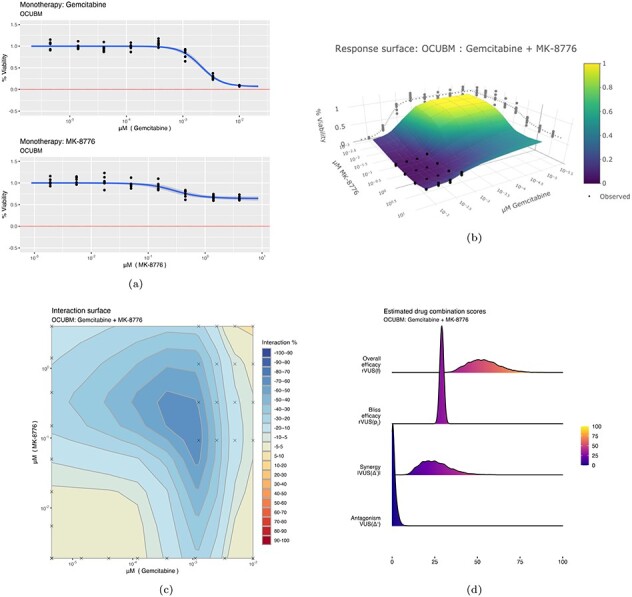
Some plots produced from the model output for the combination of Gemcitabine and MK-8776 on the OCUBM cell line. In (a), monotherapy curves for the two drugs, (b) a 3D interactive plot of the combined response, (c) contour plots of the interaction surface and in (d) posterior densities of rVUS summaries.

For the overall efficacy, rVUS() is estimated at % of the maximum available volume, with a 95% CI (37.2,72.6). Of this effect, synergy (VUS()) accounts for about 25 percentage points, 95% CI (-43.5,-11.8), whereas there is nearly no antagonistic effect at all (posterior mean of VUS() at 0.9). Note that the final estimate of synergy obtained by full MCMC sampling is larger than the initial estimate from the screen using the variational approximation. Variational inference algorithms are known for underestimating variances, which can explain why this effect was left underexplored. The wide CI in the synergy estimate is due to a large portion of the estimated effect being outside of the data range. Note that in Figure 6C, the crosses denote the observed viability locations for the drug concentrations. The large synergistic effect is supported by three or four locations in the drug concentration landscape, with the bulk of the effect taking place outside of the data range. In this region, synergy is extrapolated using the underlying smoothness assumptions of the GP, as encoded by its length-scale . The variational approximation can underestimate the variability of this smoothness parameter, and thus also synergistic effects outside of the data range. We therefore recommend that the user rerun the most interesting experiments with full MCMC to better explore the uncertainties. It would also be natural to extend this experiment with slightly smaller concentrations of the drug combination, and, in general, there is little sense in looking for synergy in areas where the monotherapies themselves are effective.

A comparison of this analysis with the results from other software packages (Table 1) is challenging due to the ‘shifted’ structure of the drug concentration grids, which creates missing observations in both the monotherapy and in the drug combination data. Both SynergyFinder 2.0 and Combenefit software packages require fully observed concentration grids to work out-of-the-box, although the online version of SynergyFinder 2.0 (https://synergyfinder.fimm.fi/) can handle missing data by integration with a separate prediction model.

The prediction model is called DECREASE [8] and utilizes a non-negative matrix factorization technique to predict a fully observed viability matrix from a sparsely observed input. After using the DECREASE model as a pre-processing step, we can thus compare bayesynergy results with the output from the SynergyFinder model. However, the DECREASE model does not handle missing observations in the monotherapies caused by the ‘shifted’ grid. In order to get around this, we first impute the missing monotherapy viabilities by using the posterior mean of a model fitted by bayesynergy, using only monotherapy viability as input. We then run the DECREASE model four times, one for each replicate of the combination viabilities, to obtain four complete dose–response matrices that can be fed into SynergyFinder. We do this in order to keep some of the data heterogeneity and ensure that SynergyFinder can provide us with confidence intervals, which requires a minimum of three replicates at each concentration.

We use the online version of both SynergyFinder 2.0 and DECREASE (https://decrease.fimm.fi/) to perform the analysis and find a synergy score based on the Bliss reference model of 11.738 0.19 for a 95% confidence interval, indicating a moderate synergistic effect. This score is calculated differently from the scores reported by the bayesynergy package, but a comparable metric can be easily computed from the posterior distribution, yielding a mean of 24.68 with a 95% CI of (11.28, 39.79). The main reason for the difference in scores and uncertainty is that the interaction surface computed by the DECREASE model quickly drops off towards zero outside the data range in all replicates, whereas the bayesynergy model uses the smoothness of the curve to extrapolate beyond the data. The predicted interaction surface from SynergyFinder, and a more detailed discussion regarding estimation uncertainty is available in Supplementary Material S7.

5.1.1 Model assessment

The interaction part of the model consists of the GP, which is constructed from the latent parameters together with the kernel hyperparameters and , and the parameters inside the transformation, . Of these, only the kernel hyperparameters can be given a clear interpretation and are therefore reported in Table 2. We see that the length-scale parameter is estimated at 1.68, 95% CI (0.96,3.09), indicating a rather smooth function over the dose concentrations that range from to 4M, also visible in Figure 6C. The kernel amplitude has a posterior mean of 3.69, with a wide 95% CI (1.32,13.35) indicating that the posterior function is allowed to deviate far from its mean, i.e. there is most likely interaction here as the function is allowed to deviate from . These parameters have a slightly smaller effective sample size, most likely due to the difficulty of updating these at the same time as updating , as reported in [22]. Although these parameters may not be of immediate interest to the user, they provide, together with the estimate of the observation noise , information about the model fit. Particularly when compared with other experiments across a large screen.

Having obtained estimates of synergy, which take the full uncertainty of the data into account, the user is left with a list of interesting experiments to follow up. Because the model properly handles the estimation uncertainty, the list of such experiments is concise, focussing on those where a true effect can be clearly differentiated from the background noise. From here, the user can analyse the drug combination screen either qualitatively by going further into the biology or quantitatively by plugging the output of the model into other algorithms for further analysis. One such avenue might be biomarker discovery models as in the style of [31], who utilizes both the efficacy estimate and its corresponding uncertainty to find biomarkers of single therapy responses. The output can also be used as training data for machine learning algorithms attempting to predict the combined drug efficacy or synergy for untested experiments.

6 Conclusion and outlook

The bayesynergy package implements a probabilistic model for analysing drug combination experiments. It handles the real world structure of drug combination experiments, which feature different patterns of missingness and differing numbers of replicates. The model accounts for measurement noise by using a heteroscedastic observation model and produces estimates of the underlying dose–response function and measures derived from it, alongside uncertainty quantification. Since the model samples from the dose–response function directly, any user-defined summary statistic of dose–response can also be computed, and the uncertainty is naturally propagated.

Through the natural grid structure of drug combination experiments, a computationally efficient GP implementation ensures the automatic exploration of the complete dose–response matrix from an incomplete input. This enables experimenters to analyse sparsely observed experiments in situations with limited resources, for example, when using patient-derived cell samples with limited biopsy material, to inform treatment decisions under uncertainty.

Cell viability assays are noisy by nature, with multiple sources of biological and technical noise. It is crucial to take this into account when estimating the efficacy and synergy of drug combinations in an attempt at understanding the underlying biological mechanisms. It enables researchers to hone in on the interesting combinations for follow up experiments and informs decision making and experimental design. More precise estimates of drug efficacy can be used as input in various models attempting to connect efficacy to underlying genomics patterns or used to predict the response in new experiments or in patients.

In this paper, we have focussed on the Bliss independence model as the underlying non-interaction assumption. This choice was motivated partly by the attractive probabilistic interpretation, but also by computational considerations. The Bliss model can be computed analytically from the two dose–response functions, whereas other models require numerical solutions (e.g. the Loewe model [1]). In an MCMC setting, this becomes expensive, as a numerical solver would need to be run at each step of the algorithm. Furthermore, both the NUTS algorithm and the variational approximation require the evaluation of the gradient of the log-posterior. Other models of non-interaction can introduce discontinuities in these gradients (e.g. the ‘Highest Single Agent’ [32]), which would make posterior sampling slow and inefficient.

An advantage of the fully Bayesian model is that the user can explore various non-interaction assumptions post hoc. From the posterior samples of the monotherapy parameters, the user can construct various non-interaction assumptions to obtain , which can then be subtracted from the posterior dose response matrix in Figure 3 to obtain . In this fashion, more suitable pharmacokinetic assumptions can be incorporated if desired. See Supplementary Material S4 for more details.

Researchers working with drug efficacy screens frequently run multiple versions of their experiments. For example, in an initial phase of setting up a large drug screen, the active ranges of various drugs might need to be determined experimentally. Sometimes entire experiments are scrapped, because they fail to meet a quality control threshold. The bayesynergy model can readily be extended to not only consider within-experiment variability, but also between-experiment variability, as in [15]. This would allow the pooling of experimental data in estimating drug efficacy and synergy, utilizing all available data for the final analysis. The differences in experimental quality can be handled by assigning different weights to different experiments according to assay quality as characterized by the positive and negative controls.

Finally, the extension of the model to higher orders of drug combinations is fairly straight forward and still computationally efficient due to the grid structure. Considering six unique concentrations for each drug, a single replicate fully observed drug combination experiment would contain 36 216 and 1296(!) viability measurements for two, three and four drugs, respectively. In these settings, resource constraints will quickly become an issue, and sparse designs an essential tool in the exploration of higher order drug synergies. In this context, we note that there is a fundamental limit on how precise measurements can be in various regions of the concentration grid (Figure 1). This is connected to the heterogeneity of cell growth and the technical error underlying cell viability assays. An avenue for further exploration is therefore the optimal design of experiments given a limited amount of resources, i.e. the optimal distribution of measurements in the concentration space and across replicates. Because the bayesynergy model samples from the full posterior distributions, we can use tools from optimal experimental design [33–35], for example, to directly minimize uncertainty in the synergy estimates.

Key Points

• Drug combination experiments are typically fraught with noise, both biological and technical.

• Accounting for this noise is key when searching for synergistic drug combinations in large screens, or when using estimates of synergy as input in other algorithms.

• The bayesynergy package implements a probabilistic model using GPs for analysing drug combination experiments, controlling for these noise sources.

• Since it is a statistical model, it allows inclusion of replicates, missing data and uneven concentration grids, in addition to providing uncertainty quantification around the results.

• By modelling the dose–response function directly, user-defined summaries of efficacy or synergy can be derived to fit individual researchers’ needs.

8 Software availability

The R package is available at https://github.com/ocbe-uio/bayesynergy. Scripts and datasets for reproducing Figures 5 and 6 and Table 2 can also be found there. All results and figures in this manuscript have been produced with the bayesynergy package version 2.4.1.

Leiv Rønneberg is a PhD student at the Oslo Centre for Biostatistics and Epidemiology working on estimation and prediction using data from drug combination experiments.

Andrea Cremaschi is Senior Researcher at the Singapore Institute for Clinical Sciences (SICS), at the Agency for Science, Technology and Research (A*STAR) in Singapore, where he works on Bayesian statistical modelling of dataset from different medical fields, including obesity, diabetes and mental health.

Robert Hanes is a Postdoctoral Researcher at Oslo University Hospital with a multidisciplinary background in information technology, medical and pharmaceutical biotechnology and biomedicine working on the development of novel and personalized treatment strategies for cancer.

Jorrit M. Enserink is a research group leader at Oslo University Hospital and Associate Professor at the University of Oslo whose research group aims to develop new strategies for cancer treatment.

Manuela Zucknick is an Associate Professor at the Oslo Centre for Biostatistics and Epidemiology at the University of Oslo, where she heads the Statistical Learning for Molecular Medicine research group.

9 Authors’ contribution statement

Initial idea by L.R., A.C. and M.Z. with further improvements and domain expertise by R.H. and J.E. Stan implementation of the model by L.R., with helper functions and plots by L.R., A.C. and R.H. L.R. and M.Z. wrote the manuscript, with reviews and comments by A.C., R.H. and J.E.

All authors have read and approved the final version of the manuscript.

References

- 1. Loewe S, Muischnek H. Uber Kombinationswirkungen. Naunyn Schmiedebergs Arch Exp Pathol Pharmakol 1926; 114:313–26. [Google Scholar]
- 2. Bliss CI. The toxicity of poisons applied jointly. Ann Appl Biol 1939; 26(3): 585–615. [Google Scholar]
- 3. Greco WR, Bravo G, Parsons JC. The search for synergy: a critical review from a response surface perspective. Pharmacol Rev 1995; 47(2): 331–85. [PubMed] [Google Scholar]
- 4. Fouquier J, Guedj M. Analysis of drug combinations: current methodological landscape. Pharmacol Res Perspect 2015; 3(3): e00149. [DOI] [PMC free article] [PubMed] [Google Scholar]
- 5. Meyer CT, Wooten DJ, Paudel BB, et al. Quantifying drug combination synergy along potency and efficacy axes. Cell Syst 2019; 8(2): 97–108. [DOI] [PMC free article] [PubMed] [Google Scholar]
- 6. Ianevski A, Giri AK, Aittokallio T. SynergyFinder 2.0: visual analytics of multi-drug combination synergies. Nucleic Acids Res 2020; 48(W1): W488–93. [DOI] [PMC free article] [PubMed] [Google Scholar]
- 7. Di Veroli GY, Fornari C, Wang D, et al. Combenefit: an interactive platform for the analysis and visualization of drug combinations. Bioinformatics 2016; 32(18): 2866–8. [DOI] [PMC free article] [PubMed] [Google Scholar]
- 8. Ianevski A, Giri AK, Gautam P, et al. Prediction of drug combination effects with a minimal set of experiments. Nat Mach Intell 2019; 1(12): 568–77. [DOI] [PMC free article] [PubMed] [Google Scholar]
- 9. Ritz C, Baty F, Streibig JC, et al. Dose-response analysis using R. PLOS ONE 2015; 10:e0146021. [DOI] [PMC free article] [PubMed] [Google Scholar]
- 10. He L, Kulesskiy E, Saarela J, et al. Methods for High-Throughput Drug Combination Screening and Synergy Scoring, Chapter 17. New York: Springer, 2018, 351–98. [DOI] [PMC free article] [PubMed] [Google Scholar]
- 11. Amzallag A, Ramaswamy S, Benes CH. Statistical assessment and visualization of synergies for large-scale sparse drug combination datasets. BMC Bioinform 2019; 20(1): 1–15. [DOI] [PMC free article] [PubMed] [Google Scholar]
- 12. Cremaschi A, Frigessi A, Taskén K, et al. A Bayesian approach for the study of synergistic interaction effects in in-vitro drug combination experiments. arXiv 2019;preprint arXiv:1904.04901. [Google Scholar]
- 13. Yadav B, Pemovska T, Szwajda A, et al. Quantitative scoring of differential drug sensitivity for individually optimized anticancer therapies. Sci Rep 2014; 4:5193. [DOI] [PMC free article] [PubMed] [Google Scholar]
- 14. Williams CK, Rasmussen CE. Gaussian Processes for Machine Learning. Cambridge, MA: MIT Press, 2006. [Google Scholar]
- 15. Hennessey VG, Rosner GL, Bast RC, et al. A Bayesian approach to dose-response assessment and synergy and its application to in vitro dose-response studies. Biometrics 2010; 66(4): 1275–83. [DOI] [PMC free article] [PubMed] [Google Scholar]
- 16. Tansey W, Li K, Zhang H, et al. Dose–response modeling in high-throughput cancer drug screenings: an end-to-end approach. Biostatistics 2021: kxaa047. [DOI] [PMC free article] [PubMed] [Google Scholar]
- 17. Zhang J-H, Chung TDY, Oldenburg KR. A simple statistical parameter for use in evaluation and validation of high throughput screening assays. J Biomol Screen 1999; 4(2): 67–73. [DOI] [PubMed] [Google Scholar]
- 18. Carpenter B, Gelman A, Hoffman MD, et al. A probabilistic programming language. J Stat Softw 2017; 76(1): 1–32. [DOI] [PMC free article] [PubMed] [Google Scholar]
- 19. Stan Development Team . RStan: The R Interface to Stan. R package version 2.21.2, 2020.
- 20. Hoffman MD, Gelman A. The No-U-Turn sampler: adaptively setting path lengths in Hamiltonian Monte Carlo. J Mach Learn Res 2014; 15(47): 1593–623. [Google Scholar]
- 21. Kucukelbir A, Ranganath R, Gelman A, et al. Automatic variational inference in Stan. In: Advances in Neural Information Processing Systems. 2015; 2015: 568–76.
- 22. Flaxman S, Gelman A, Neill D, et al. Fast hierarchical Gaussian processes, 2015. Manuscript in preparation. Available online at http://sethrf.com/files/fast-hierarchical-GPs.pdf.
- 23. Shehata M, Schnabl S, Demirtas D, et al. Reconstitution of PTEN activity by CK2 inhibitors and interference with the PI3-K/Akt cascade counteract the antiapoptotic effect of human stromal cells in chronic lymphocytic leukemia. Blood 2010; 116(14): 2513–21. [DOI] [PubMed] [Google Scholar]
- 24. O’Neil J, Benita Y, Feldman I, et al. An unbiased oncology compound screen to identify novel combination strategies. Mol Cancer Ther 2016; 15(6): 1155–62. [DOI] [PubMed] [Google Scholar]
- 25. Liu H, Zhang W, Zou B, et al. DrugCombDB: a comprehensive database of drug combinations toward the discovery of combinatorial therapy. Nucleic Acids Res 2019; 48(D1): D871–D881. [DOI] [PMC free article] [PubMed] [Google Scholar]
- 26. Kass RE, Raftery AE. Bayes factors. J Am Stat Assoc 1995; 90(430): 773–95. [Google Scholar]
- 27. Gronau QF, Singmann H, Wagenmakers E-J. bridgesampling: an R package for estimating normalizing constants. J Stat Softw 2020; 92(10): 1–29. [Google Scholar]
- 28. Choi M, Kipps T, Kurzrock R. ATM mutations in cancer: therapeutic implications. Mol Cancer Ther 2016; 15(8): 1781–91. [DOI] [PubMed] [Google Scholar]
- 29. Daud AI, Ashworth MT, Strosberg J, et al. Phase I dose-scalation trial of checkpoint kinase 1 inhibitor MK-8776 as monotherapy and in combination with gemcitabine in patients with advanced solid tumors. J Clin Oncol 2015; 33(9): 1060–6. [DOI] [PubMed] [Google Scholar]
- 30. Origanti S, Cai SR, Munir AZ, et al. Synthetic lethality of Chk1 inhibition combined with p53 and/or p21 loss during a DNA damage response in normal and tumor cells. Oncogene 2012; 32(5): 577–88. [DOI] [PMC free article] [PubMed] [Google Scholar]
- 31. Wang D, Hensman J, Kutkaite G, et al. A statistical framework for assessing pharmacological responses and biomarkers using uncertainty estimates. eLife 2020; 9: e60352. [DOI] [PMC free article] [PubMed] [Google Scholar]
- 32. Lehár J, Zimmermann GR, Krueger AS, et al. Chemical combination effects predict connectivity in biological systems. Mol Syst Biol 2007; 3(1): 80. [DOI] [PMC free article] [PubMed] [Google Scholar]
- 33. Chou TC. Theoretical basis, experimental design, and computerized simulation of synergism and antagonism in drug combination studies. Pharmacol Rev 2006; 58(3): 621–81. [DOI] [PubMed] [Google Scholar]
- 34. Chaloner K, Verdinelli I. Bayesian experimental design: a review. Stat Sci 1995; 10(3): 273–304. [Google Scholar]
- 35. Holland-Letz T, Kopp-Schneider A. Optimal experimental designs for dose–response studies with continuous endpoints. Arch Toxicol 2014; 89(11): 2059–68. [DOI] [PMC free article] [PubMed] [Google Scholar]
- 36. Menden MP, Wang D, Mason MJ, et al. Community assessment to advance computational prediction of cancer drug combinations in a pharmacogenomic screen. Nat Commun 2019; 10(1): 1–17. [DOI] [PMC free article] [PubMed] [Google Scholar]
Associated Data
This section collects any data citations, data availability statements, or supplementary materials included in this article.