Fast mesh data augmentation via Chebyshev polynomial of spectral filtering

Abstract

Deep neural networks have recently been recognized as one of the powerful learning techniques in computer vision and medical image analysis. Trained deep neural networks need to be generalizable to new data that are not seen before. In practice, there is often insufficient training data available, which can be solved via data augmentation. Nevertheless, there is a lack of augmentation methods to generate data on graphs or surfaces, even though graph convolutional neural network (graph-CNN) has been widely used in deep learning. This study proposed two unbiased augmentation methods, Laplace–Beltrami eigenfunction Data Augmentation (LB-eigDA) and Chebyshev polynomial Data Augmentation (C-pDA), to generate new data on surfaces, whose mean was the same as that of observed data. LB-eigDA augmented data via the resampling of the LB coefficients. In parallel with LB-eigDA, we introduced a fast augmentation approach, C-pDA, that employed a polynomial approximation of LB spectral filters on surfaces. We designed LB spectral bandpass filters by Chebyshev polynomial approximation and resampled signals filtered via these filters in order to generate new data on surfaces. We first validated LB-eigDA and C-pDA via simulated data and demonstrated their use for improving classification accuracy. We then employed brain images of the Alzheimer’s Disease Neuroimaging Initiative (ADNI) and extracted cortical thickness that was represented on the cortical surface to illustrate the use of the two augmentation methods. We demonstrated that augmented cortical thickness had a similar pattern to observed data. We also showed that C-pDA was faster than LB-eigDA and can improve the AD classification accuracy of graph-CNN.

1. Introduction

Deep neural networks have recently been recognized as one of the powerful learning techniques in computer vision and medical image analysis (Litjens et al., 2017; Shen, Wu, & Suk, 2017). Training deep neural networks requires a large dataset so that they are generalizable to data that have never been seen before. This is challenging especially in the field of medical image analysis. Building big medical image datasets is expensive and labor-intensive to collect, and is related to patient privacy, and requires medical experts for labeling. Not having enough data could overfit training data so that network models are not generalized to new data. Moreover, studies on rare diseases or medical screening also face the problem of class imbalance with a skewed ratio of majority to minority samples (Ker, Wang, Rao, & Lim, 2017; Mazurowski et al., 2008). These obstacles have led to many studies on image data augmentation (see review in Leevy, Khoshgoftaar, Bauder, & Seliya, 2018). Data augmentation assumes that additional information can be extracted from an original dataset. It is a very powerful approach for overcoming overfitting in deep learning.

Image augmentation inflates the size of training data via either image transformation or oversampling. New images can be generated by warping existing images via geometric (rotation, flipping) and color transformations (Shorten & Khoshgoftaar, 2019), random erasing (Zhong, Zheng, Kang, Li, & Yang, 2017), and adversarial training (Ganin et al., 2016; Goodfellow, Shlens, & Szegedy, 2014) such that their labels are preserved. In contrast, oversampling augmentation creates synthetic data by mixing existing images, auto encoder–decoder (DeVries & Taylor, 2017; Kingma & Welling, 2013), and generative adversarial networks (GANs) (Goodfellow et al., 2014; Yi, Walia, & Babyn, 2019). Even though GANs are powerful, their computation is more expensive compared to image warping methods.

Among existing image augmentation methods (DeVries & Taylor, 2017; Goodfellow et al., 2014; Kingma & Welling, 2013; Shorten & Khoshgoftaar, 2019; Yi et al., 2019; Zhong et al., 2017), image data are defined on an equi-spaced grid in the Euclidean space. However, medical images in the Euclidean space may not fully characterize the geometry of human organs that encompass their intrinsic and complex anatomy, as well as physiological functions. For example, the cerebral cortex is composed of ridges (gyri) and valleys (sulci). Due to the way gyri and sulci are curved, the cortex is thicker in gyri but thinner in sulci. Hence, it is preferred to represent brain images in a way that the underlying geometrical information is encoded. One can express the cerebral cortex as a surface embedded in the 3D Euclidean space. Existing literature has demonstrated that such representation incorporates useful geometry information of the brain into machine learning for disease diagnosis (Apostolova et al., 2006; Fan et al., 2008; Qiu, Fennema-Notestine, Dale, Miller, & the Alzheimer’s Disease Neuroimaging Initiative, 2009; Yang, Goh, Chen, & Qiu, 2013). Recently, a number of deep neural networks, such as diffusion-convolutional neural networks (DC-NNs) (Atwood & Towsley, 2015), PATCHY-SAN (Duvenaud et al., 2015; Niepert, Ahmed, & Kutzkov, 2016), gated graph sequential neural networks (Li, Tarlow, Brockschmidt, & Zemel, 2015), DeepWalk (Perozzi, Al-Rfou, & Skiena, 2014), and spectral graph convolutional neural networks (graph-CNN) (Bruna, Zaremba, Szlam, & LeCun, 2013; Defferrard, Bresson, & Vandergheynst, 2016; Henaff, Bruna, & LeCun, 2015; Kipf & Welling, 2016; Ktena et al., 2017; Shuman, Ricaud, & Vandergheynst, 2016; Yi, Su, Guo, & Guibas, 2017) can take data on surfaces for classification. The core challenge for implementing CNN on surfaces lies in defining convolution on surfaces. These existing neural network approaches focus on how to process vertices whose neighborhood has different sizes and connections for the convolution in the spatial domain. Alternately, convolution can be defined as a multiplication involving a diagonal matrix in the graph Fourier transform derived from a normalized graph Laplacian in the spectral domain. Hence, existing image warping augmentations on equi-spaced grids (e.g., flipping, rotation, shifting) may not directly apply to data on surfaces since the points on surfaces are not on the equi-spaced grid of the Euclidean space. Nevertheless, there is a lack of augmentation approaches to generate data on surfaces.

This study proposed two unbiased augmentation methods, Laplace–Beltrami eigenfunction Data Augmentation (LB-eigDA) and Chebyshev polynomial Data Augmentation (C-pDA), to generate new data on surfaces. These two approaches preserved the mean of observed data in each class, which is crucial for classification problems. These two approaches were motivated by the Fourier representation of signals in equi-spaced Euclidean grids. A signal in equi-spaced Euclidean grids can be created as a linear combination of Fourier bases, where the corresponding Fourier coefficients can be generated via the resampling of the Fourier coefficients of existing signals (Ravanbakhsh, Schneider, & Poczos, 2016; Tang, 2013; Wang, Ombao, & Chung, 2018). We adopted this idea and computed the eigenfunctions of the Laplace–Beltrami (LB) operator on a surface. New data on the surface can be constructed via the resampling of the LB coefficients among observed data on the surface.

In parallel with LB-eigDA, we introduced a fast augmentation approach, C-pDA, that employed a polynomial approximation of LB spectral filters on surfaces. C-pDA was designed to be in line with graph-CNN (Defferrard et al., 2016; Shuman et al., 2016), where spectral filters were implemented via Chebyshev polynomial approximation such that the resulting convolution can be written as a polynomial of the adjacency matrix of a graph. This avoided the cost of calculating the eigenfunctions of a large-scale graph Laplacian. In Defferrard et al. (2016) and Shuman et al. (2016), it was shown that the kth order Chebyshev polynomial formation of the graph Laplacian is equivalent to k-ring filtering. In C-pDA, we designed LB spectral bandpass filters by Chebyshev polynomial approximation and resampled filtered observed data to generate new data. Due to the recurrence relation of Chebyshev polynomials, the computation of the C-pDA method can be efficient. We validated LB-eigDA and C-pDA using simulated data with the ground truth of class labels. We further employed the methods to the cortical surface data in the Alzheimer’s Disease Neuroimaging Initiative (ADNI). We first demonstrated that augmented cortical thickness data had a similar pattern to observed data. Second, we showed that C-pDA was much faster than LB-eigDA. Last, we illustrated the use of C-pDA to improve the AD classification of the graph-CNN (Defferrard et al., 2016).

The main contributions of this study were as follows.

• We introduced two augmentation methods to generate new data on surfaces using the LB eigenfunctions and LB spectral filters.

• We showed that C-pDA was computationally more efficient than LB-eigDA.

• We demonstrated that C-pDA improved the graph-CNN performance on the classification of AD patients.

2. Methods

In the field of medical image analysis, triangulated surface meshes are often used to represent the geometry of cells, tissue and organs. They are generated from 3D segmented images and comprised of vertices and edges. In the following, we will introduce LB-eigDA (Fig. 1) and C-pDA (Fig. 2) methods for generating new data on such triangulated surface meshes. We will employ the Laplace–Beltrami (LB) operator due to its incorporation of the intrinsic geometry of triangulated surface meshes.

Fig. 1.

Flowchart of the proposed LB-eigDA method for generating n augmented samples from n observations (original samples) on a hippocampus triangulated surface mesh. The hippocampal surface is represented by a triangulated mesh with 1184 vertices and 2364 triangles.

Fig. 2.

Flowchart of the proposed C-pDA method for generating n augmented samples from n observations (original samples) on a hippocampus triangulated surface mesh. The hippocampal surface is represented by a triangulated mesh with 1184 vertices and 2364 triangles.

2.1. Augmentation based on the Laplace–Beltrami representation of signals on a surface mesh

We introduce a data augmentation method based on the LB representation of signals on a surface mesh. We denote the surface as $\mathcal{M}$ with the LB-operator ∆ on $\mathcal{M}$. Let ψ_j be the jth eigenfunction of the LB-operator with eigenvalue λ_j

$$\mathit{\Delta }{\psi }_j={\lambda }_j{\psi }_j,$$ (1)

where 0 = λ₀ ≤ λ₁ ≤ λ₂ ≤ ⋯. A signal f (x) on the surface $\mathcal{M}$ can be represented as a linear combination of the LB eigenfunctions

$$f\left(x\right)=\sum _{j=0}^{\infty }{c}_j{\psi }_j\left(x\right),$$ (2)

where c_j is the jth coefficient associated with the eigenfunction ψ_j(x). Consider n observations (real samples), f₁(x), …, f_n(x). The ith observation f_i(x) can be represented as

$$f_i\left(x\right)=\sum _{j=0}^{\infty }{c}_j^{\left(i\right)}{\psi }_j\left(x\right),$$

where $c_j^{\left(i\right)}$ is the jth coefficient associated with the jth LB eigenfunction for the ith observation. We like to generate new data based on the frequency resampling of these n observations. This is similar to creating new samples via permuting Fourier coefficients (Wang et al., 2018). Let S_n be the permutation group of order n (Chung et al., 2019) and τ ∈ S_n be an element of permutation given by

$$\tau =\left(\begin{array}{cccc}1& 2& \cdots & n\\ \tau \left(1\right)& \tau \left(2\right)& \cdots & \tau \left(n\right)\end{array}\right).$$ (3)

τ (i) indicates that element i is permuted to τ (i). We resample the LB coefficients to obtain new data, and the i′th augmented sample ${\tilde{f}}_{i\prime }\left(x\right)$ can be written as:

$${\tilde{f}}_{i\prime }\left(x\right)=\sum _{j=0}^{\infty }{c}_j^{{\tau }_j\left(i\right)}{\psi }_j\left(x\right),$$ (4)

where τ_j(·) is the permutation on the jth LB coefficients among the n observations. We will refer this approach as LB eigenfunction Data Augmentation (LB-eigDA). Fig. 1 illustrates the flowchart of the LB-eigDA.

Based on Eq. (4), one can show that the mean of ${\tilde{f}}_{i\prime }\left(x\right)$ over every possible permutation is the same as that of observed f_i(x) since the permutation function τ (·) does not change the mean of the LB coefficients.

2.2. Augmentation via Chebyshev polynomials

Previous research suggests that the augmentation strategy of Gaussian filters leads to the best validation accuracy in medical imaging classification tasks (Hussain, Gimenez, Yi, & Rubin, 2017). We now introduce the second data augmentation approach, Chebyshev polynomial Data Augmentation (C-pDA). As illustrated in Fig. 2, the idea of C-pDA is similar to the augmentation strategy of Gaussian filters in equi-spaced grids of the Euclidean space by designing LB spectral filters on surfaces. We design LB spectral filters that are similar to spectral filter banks (Tan & Qiu, 2015). We can then approximate observed data on surfaces using these LB spectral filters and resample the LB spectral filtered signals of observed data in order to generate new data on surfaces. To avoid the direct computation of the LB eigenfunctions, we will employ the Chebyshev polynomial approximation of LB spectral filters, which is computationally efficient. In the following, we first describe the Chebyshev polynomial approximation of an LB spectral filter and then design LB spectral bandpass filters for the C-pDA approach.

2.2.1. Chebyshev polynomial approximation of LB spectral filters

Consider an LB spectral filter g on the surface $\mathcal{M}$ with spectrum g (λ) as

$$g\left(x,y\right)=\sum _{j=0}^{\infty }g\left({\lambda }_j\right){\psi }_j\left(x\right){\psi }_j\left(y\right).$$ (5)

Based on Eq. (2), the convolution of a signal f with the filter g can be written as

$$h\left(x\right)=g\hspace{0.17em}\ast \hspace{0.17em}f\left(x\right)=\sum _{j=0}^{\infty }g\left({\lambda }_j\right)c_j{\psi }_j\left(x\right).$$ (6)

As suggested in Coifman and Maggioni (2006), Defferrard et al. (2016), Hammond, Vandergheynst, and Gribonval (2011), Kim et al. (2012), Tan and Qiu (2015) and Wee et al. (2019), the filter spectrum g (λ) in Eq. (6) can be represented as the expansion of Chebyshev polynomials, T_k, k = 0, 1, 2, …, ∞, such that

$$g\left(\lambda \right)=\sum _{k=0}^{\infty }{\theta }_k{T}_k\left(\lambda \right).$$ (7)

θ_k is the kth expansion coefficient associated with the kth Chebyshev polynomial. T_k is the Chebyshev polynomial of the form T_k(λ) = cos(k cos⁻¹ λ) with recurrence

$$T_{k+1}\left(\lambda \right)=\left(2-{\delta }_{k0}\right)\lambda \hspace{0.17em}{T}_k\left(\lambda \right)-T_{k-1}\left(\lambda \right),$$

where δ_k0 is Kronecker delta. The convolution in Eq. (6) can be rewritten as

$$h\left(x\right)=g\hspace{0.17em}\ast \hspace{0.17em}f\left(x\right)=\sum _{k=0}^{\infty }{\theta }_k{T}_k\left(\mathit{\Delta }\right)f\left(x\right).$$ (8)

This Chebyshev polynomial approximation of the spectral filter has previously used in diffusion wavelet transform (Coifman & Maggioni, 2006; Donnat, Zitnik, Hallac, & Leskovec, 2018; Hammond et al., 2011; Kim et al., 2012), graph convolutional neural network (Defferrard et al., 2016; Wee et al., 2019), spectral wavelet transform (Tan & Qiu, 2015), and heat diffusion (Huang, Lyu, Qiu, & Chung, 2020) on graphs. The polynomial method avoids the direct computation of the LB eigenfunctions through the recursive computation of T_k(∆)f (x) and preserves local geometric structure of the surface (Defferrard et al., 2016; Huang et al., 2020).

2.2.2. C-pDA

We design a series of LB spectral bandpass filters, g_l, l = 1, 2, …, L, based on Eq. (7) such that

$$g_l\left(\lambda \right)=\sum _{k=0}^{\infty }{\theta }_{lk}{T}_k\left(\lambda \right)$$

where θ_lk is the kth Chebyshev expansion coefficient of the lth bandpass filter. The frequency band of the lth bandpass filter is $\lambda \in \left[{ϵ}_l\hspace{0.17em}{ϵ}_{l+1}\right]$. Now, a signal f (x) on surface $\mathcal{M}$ can be approximated using these filters such that

$$f\left(x\right)\approx h_0+\sum _{l=1}^L{g}_l\left(\mathit{\Delta }\right)f\left(x\right),$$ (9)

where h₀ is the mean of f (x) over the surface. If g_l, l = 1, 2, …, L, together span the entire spectrum of f (x), then the spectral information of f (x) is retained.

We develop the C-pDA approach in a way similar to the LB-eigDA approach in Eq. (4) such that the i′th augmented sample ${\tilde{f}}_{i\prime }\left(x\right)$ can be written as

$${\tilde{f}}_{i\prime }\left(x\right)=h_0^{{\tau }_0\left(i\right)}+\sum _{l=0}^L{\left(g_l\left(\mathit{\Delta }\right)f_i\left(x\right)\right)}^{{\tau }_l\left(i\right)},$$ (10)

where τ_l(·) is the permutation on the lth filtered signal among the n observations (real samples) f₁, f₂, …, f_n such that the ith observation is permuted to the τ_l(i)th observation. Hence, C-pDA generates new data via resampling the lth filtered outputs among the n observations and summing the resampled signals across L filters. Again, we can show that the mean of ${\tilde{f}}_{i\prime }\left(x\right)$ over every possible permutation is the same as that of f_i(x) since the permutation function τ (·) does not change the mean of the filtered signals.

With the Chebyshev polynomial approximation, we can rewrite Eq. (10) as

$${\tilde{f}}_{i\prime }\left(x\right)=h_0^{{\tau }_0\left(i\right)}+{\sum _{l=1}^L\left(\sum _{k=0}^{\infty }{\theta }_{lk}{T}_k\left(\mathit{\Delta }\right)f_i\left(x\right)\right)}^{{\tau }_l\left(i\right)}.$$ (11)

2.3. LB-eigDA and C-pDA numerical implementation

For the implementation of the LB-eigDA in Eq. (4), we adopt the discretization scheme of the LB-operator in Tan and Qiu (2015), where surface $\mathcal{M}$ is represented by a triangulated mesh with a set of triangles and vertices v_i. The ijth element of the LB-operator on $\mathcal{M}$ can be computed as

$${\mathit{\Delta }}_{ij}={\text{C}}_{ij}/A_i,$$ (12)

where A_i is estimated by the Voronoi area of nonobtuse triangles (Meyer, Desbrun, Schröder, & Barr, 2003) and the Heron’s area of obtuse triangles containing v_i (Meyer et al., 2003; Tan & Qiu, 2015). The off-diagonal entries are defined as $C_{ij}=-\left(\cot {\theta }_{ij}+\cot {\varphi }_{ij}\right)/2$ if v_i and v_j form an edge, otherwise C_ij = 0. The diagonal entries C_ii are computed as $C_{ii}=-{\sum }_j{C}_{ij}$. Other cotan discretizations of the LB-operator are discussed in Chung, Qiu, Seo, and Vorperian (2015), Chung and Taylor (2004) and Qiu, Bitouk, and Miller (2006). When the number of vertices on $\mathcal{M}$ is large, the computation of the LB eigenfunctions can be costly (Huang et al., 2020).

For the numerical implementation of the C-pDA method in Eq. (11), we need to first determine the order of Chebyshev polynomials while g_l(λ) have less overlap for C-pDA. One can quantify the overlap among the filters g_l via training the spectral band between the passband and stopband (Oppenheim, Schafer, & Buck, 1999). A higher-order filter has a narrower transition band than a lower-order filter. Fig. 3 shows the transition bandwidth over order K for Chebyshev polynomials when the filter band is λ ∈ [0.05λ_max, 0.1λ_max], where λ_max is the maximum eigenvalue of the LB-operator. In this study, we empirically determined the order of Chebyshev polynomials as K = 5000 for C-pDA, which achieves the transition bandwidth as small as 3.5 × 10⁻⁴ as illustrated in Fig. 3. L depends on the spectral distribution of the observations and thus is application-specific. This study empirically determines L in the below applications.

Fig. 3.

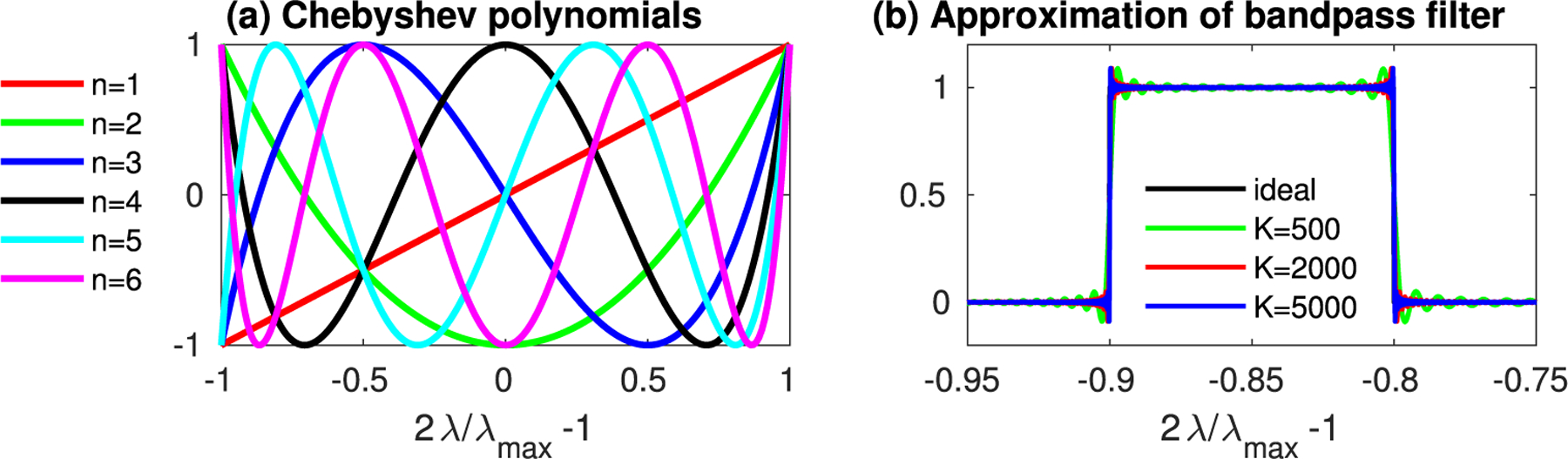
(a) Chebyshev polynomials of order 1 to 6. (b) An ideal rectangular bandpass filter with range λ ∈ [0.05λ_max, 0.1λ_max] and its approximation of Chebyshev polynomials of order up to K = 500, 2000, and 5000.

We take the advantage of the recurrence relation of the Chebyshev polynomials and compute C-pDA recursively. We now describe steps for the numerical implementation of Eq. (11).

1. discretize the surface $\mathcal{M}$ using a triangulated mesh;

2. compute ∆ based on Eq. (12) for the surface mesh $\mathcal{M}$;

3. compute the maximum eigenvalue λ_max of ∆. For the standardization across surface meshes, we normalize ∆ as $\tilde{\mathit{\Delta }}=\frac{2\mathit{\Delta }}{{\lambda }_{\max }}-I$, where I is an identity matrix;

4. for the signal f_i of the ith subject, compute $T_k\left(\tilde{\mathit{\Delta }}\right)f_i\left(x\right)$ recursively by

   $$T_{k+1}\left(\tilde{\mathit{\Delta }}\right)f_i\left(x\right)=\left(2-{\delta }_{k0}\right)\tilde{\mathit{\Delta }}{T}_k\left(\tilde{\mathit{\Delta }}\right)f_i\left(x\right)-T_{k-1}\left(\tilde{\mathit{\Delta }}\right)f_i\left(x\right)$$

   with initial conditions

   $$T_{-1}\left(\tilde{\mathit{\Delta }}\right)f_i\left(x\right)=0$$

   and

   $$T_0\left(\tilde{\mathit{\Delta }}\right)f_i\left(x\right)=f_i\left(x\right).$$
5. compute each augmented signal ${\tilde{f}}_{i\prime }$ recursively as

   $${\tilde{f}}_{i\prime }^k\left(x\right)={\tilde{f}}_{i\prime }^{k-1}\left(x\right)+\sum _{l=0}^L{\left({\theta }_{lk}{T}_k\left(\tilde{\mathit{\Delta }}\right)f_i\left(x\right)\right)}^{{\tau }_l\left(i\right)},$$

   where

   $${\theta }_{lk}=\frac{2-{\delta }_{k0}}{\pi }{\int }_{{ϵ}_k}^{{ϵ}_{k+1}}{T}_k\left(\lambda \right)\frac{d\lambda }{\sqrt{1-{\lambda }^2}},$$

   where $\left[{ϵ}_k\hspace{0.17em}{ϵ}_{k+1}\right]$ is the frequency band of g_l. Steps 4 and 5 are repeated from k = 0 till k = K − 1. In step 5, there is no need to explicitly compute each filtered signal, which saves computational time and memory, especially when a large number of filters are used.

The code of both methods are available at (https://github.com/bieqa/Surface-Data-Augmentation).

3. Simulation experiments

A majority of medical applications often face two challenges, limited sample sizes and potential uncertainty of diagnosis (Ranginwala, Hynan, Weiner, & White III, 2008; Tong et al., 2014). We designed simulation experiments with the ground truth of group labels to illustrate the use of LB-eigDA and C-pDA in the sample size estimation and diagnosis classification.

We performed simulation experiments using a hippocampus surface mesh with 1184 vertices and 2364 triangles. We generated two groups of simulated data on this surface mesh: n samples in Group 0 and m samples in Group 1. We first generated n + m measurements by a normal distribution with mean 0 and variance σ ², i.e., $\mathcal{N}\left(0,{\sigma }^2\right)$, at each vertex of the hippocampus surface. The first n measurements were considered as samples in Group 0, while the rest of m measurements were added signal 1 in a small patch on the hippocampus (see the red region in Fig. 4(a)) and were considered as Group 1. Thus, Group 0 had the distribution $\mathcal{N}\left(0,{\sigma }^2\right)$ at each vertex, while Group 1 had the distribution $\mathcal{N}\left(1,{\sigma }^2\right)$ in the small patch of the hippocampus and the distribution of $\mathcal{N}\left(0,{\sigma }^2\right)$ at each vertex on the rest of the hippocampus. Fig. 4(a) shows the signal averaged over 500 samples in Group 1.

Fig. 4.

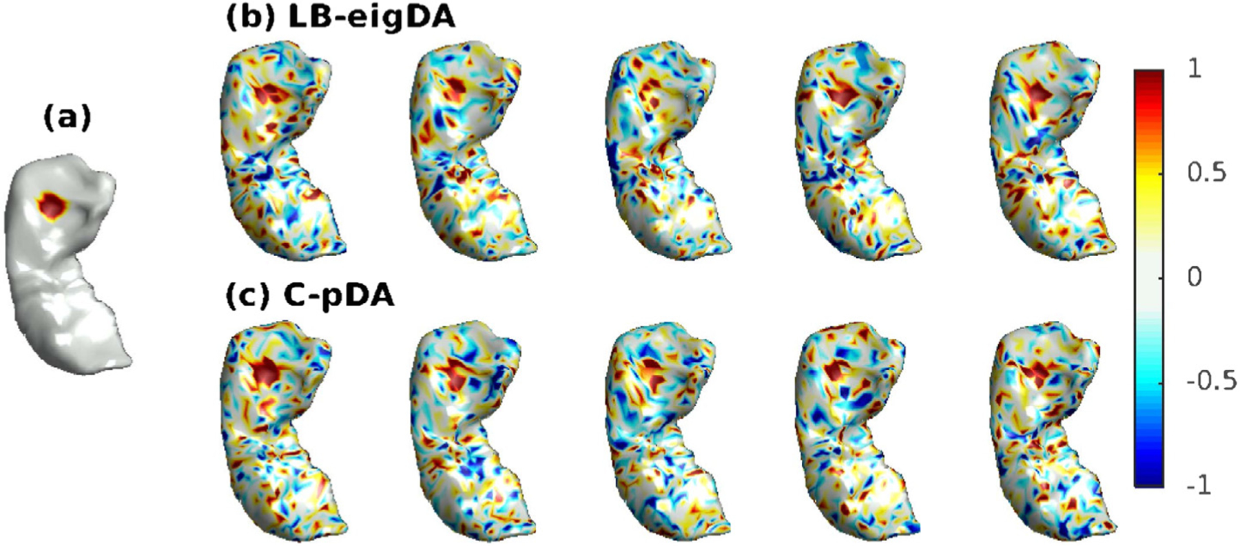
Simulated and augmented data in Group 1. (a) Averaged signal over 500 samples that were simulated via the distribution $\mathcal{N}\left(1,{\sigma }^2\right)$ in the small patch (red region) of the hippocampus and the distribution of $\mathcal{N}\left(0,{\sigma }^2\right)$ at each vertex on the rest of the hippocampus. (b) five augmented samples for Group 1 via the LB-eigDA method; and (c) five augmented samples for Group 1 via the C-pDA method.

To generate augmented data, we computed all the 1184 eigenfunctions for LB-eigDA. The hippocampal surface mesh had the spectrum over [0, 10.9]. For C-pDA, we used 109 bandpass filters whose bandwidth was 0.1 and a mean filter that computed the average value of a signal over the hippocampal surface. Each filter was approximated by Chebyshev polynomials of order 5000. Fig. 4(b) and (c) show 5 augmented samples generated by LB-eigDA and C-pDA for Group 1, respectively.

We employed a convolutional neural network (CNN) that was a modified version of the graph-CNN in Defferrard et al. (2016) and Wee et al. (2019). We employed the LB-operator instead of the graph Laplacian in the CNN in this study. We called it an LB-based spectral CNN. Fig. 5 shows the LB-based spectral CNN architecture with two convolutional layers due to the relatively small surface mesh of the hippocampus and one fully connected layer. The two convolutional layers had 8 and 16 filters, respectively. Each filter was characterized by the Chebyshev polynomials of order 7. Moreover, each layer also included a rectified linear unit (ReLU) and average pooling. We trained the network with an initial learning rate of 10⁻³, and a learning rate decay of 0.05 for every 20 epochs. We applied the ten-fold cross-validation, where one fold was used for testing and the other 9 folds were for training (75%) and validation (25%). Fig. 7 (a) shows the classification accuracy versus total sample size n + m with ratio n/m = 2, which was similar to real ADNI data used below in this study. σ = 0.6 was used. A higher value of σ resulted in a similar curve except that more samples were required to reach the same classification accuracy. The accuracy reached 98.1% when the total sample size was 3000 and then increased slowly as the sample size increased.

Fig. 5.

The LB-based spectral CNN with 2 convolutional layers and one fully connected layer. Each convolutional layer is comprised of filters approximated by the Chebyshev polynomials of order 7, a rectified linear unit (ReLU), and average pooling.

Fig. 7.

Classification accuracy on simulated and augmented data. (a) The classification accuracy using simulated data when the sample size increased from 300 to 9000. (b) The green dotted line shows the classification accuracy when only X% of simulated data was used as the training set. The red dashed and blue solid lines show the classification accuracy when only X% of the training set were simulated data and 1 − X% of the training set were augmented data by the LB-eigDA and C-pDA methods, respectively.

To demonstrate the use of the two augmentation methods in classification, we fixed the total sample size as 3000 (n = 2000, m = 1000). Among the 3000 samples, 2025, 675, and 300 samples were respectively used as the training, validation, and testing samples. As illustrated in Fig. 6, when only a smaller fraction of the simulated data in the training, denoted as X%, was available, we applied the augmentation methods to add 1 − X% augmented data to the training set. For instance, if X = 10, we only used 203 of the training samples and employed LB-eigDA or C-pDA to generate 1822 augmented samples as additional training samples. The augmentation was employed separately for the two groups. The validation (675 samples) and testing (300 samples) sets remained the same. The classification accuracy was respectively 95.5% for LB-eigDA and 92.5% for C-pDA. Without the augmented data, the classification accuracy was 80.3%, more than 10% lower than that obtained using the data augmented by LB-eigDA and C-pDA. Fig. 7 (b) shows that LB-eigDA and C-pDA improved the classification accuracy when compared to that without augmented data. Moreover, the LB-eigDA method performed in general better than the C-pDA method. This is mainly because the C-pDA method employs the polynomial approximation of the LB spectral filters.

Fig. 6.

Real and augmented data used in the LB-based spectral CNN. X% indicates that the percentage of the training set is real data and 1 − X% are augmented data.

4. Results

We used MRI data from ADNI. We first illustrate the similarity of augmented data by LB-eigDA and C-pDA to real MRI data. We then compare the computational cost of the LB-eigDA and C-pDA approaches. Finally, we show the use of C-pDA in the LB-based spectral CNN to improve the classification accuracy of Alzheimer’s patients.

4.1. MRI data acquisition and preprocessing

We used ADNI-2 cohort (adni.loni.ucla.edu) acquired from participants aging from 55 to 90 using either 1.5 or 3T scanners. For the typical 1.5T acquisition, repetition time (TR) = 2400 ms, minimum full echo time (TE) and inversion time (TI)= 1000 ms, flip angle= 8°, field-of-view (FOV)= 240 × 240 mm², acquisition matrix = 256 × 256 × 170 in the x-, y-, and z-dimensions, yielding a voxel size of 1.25 × 1.25 × 1.2 mm³. For the 3T scans, TR= 2300 ms, minimum full TE and TI = 900 ms, flip angle= 8°, FOV= 260 × 260 mm², acquisition matrix = 256 × 256 × 170, yielding a voxel size of 1.0 × 1.0 × 1.2 mm³.

We utilized the structural T1-weighted MRI from the ADNI-2 dataset. The number of visits of each subject varied from 1 to 7 (i.e., baseline, 3-, 6-, 12-, 24-, 36-, and 48-month), and at each visit, the subjects were diagnosed with one of the four clinical statuses based on the criteria in the ADNI protocol (adni.loni.ucla.edu): healthy control (HC), early mild cognitive impairment (MCI), late MCI, and Alzheimer’s disease (AD). In this study, we illustrated the use of the augmentation methods via the HC/AD classification since it has been well studied using T1-weighted image data (e.g. Basaia et al., 2019; Cuingnet et al., 2011; Hosseini-Asl, Keynton, & El-Baz, 2016; Islam & Zhang, 2018; Korolev, Safiullin, Belyaev, & Dodonova, 2017; Liu et al., 2013; Liu, Zhang, Adeli, & Shen, 2018; Wee et al., 2019). Hence, this study involved 643 subjects with HC or AD scans (392 subjects had HC scans; 253 subjects had AD scans). There were 8 subjects who fell into both groups due to the conversion from HC to AD. Table 1 lists the demographic information of the ADNI-2 cohort.

Table 1.

Demographic information of the ADNI-2 cohort with MRI scans.

	HC	AD
The number of subjectsa	400	261
The number of scans	1122	587
Gender (female/male)	607/515	254/333
Age (years; mean±SD)	75.3 ± 6.8	75.3 ± 7.7

^aThere are 8 subjects who fall into both the HC and AD groups due to the conversion from HC to AD. Abbreviations: HC, healthy controls; AD: Alzheimer’s disease; SD, standard deviation.

The T1-weighted images were segmented using FreeSurfer (version 5.3.0) (Fischl et al., 2002). The white and pial cortical surfaces were generated at the boundary between white and gray matter and the boundary of gray matter and CSF, respectively. Cortical thickness was computed as the distance between the white and pial cortical surfaces. It represents the depth of the cortical ribbon. We represented cortical thickness on the mean surface, the average between the white and pial cortical surfaces. We employed large deformation diffeomorphic metric mapping (LDDMM) (Du, Younes, & Qiu, 2011; Zhong, Phua, & Qiu, 2010) to align individual cortical surfaces to the atlas and transferred the cortical thickness of each subject to the atlas. The cortical atlas surface was represented as a triangulated mesh with 655,360 triangles and 327,684 vertices. At each surface vertex, a spline regression implemented by piecewise step functions (James, Witten, Hastie, & Tibshirani, 2013) was performed to regress out the effects of age and gender. The residuals from the regression were used in the below LB-based spectral CNN.

4.2. LB-eigDA and C-pDA augmentation

We extracted cortical thickness data from 500 ADNI brain MRI scans and then used them to generate augmented cortical thickness via LB-eigDA and C-pDA.

C-pDA requires determining the number of filters and the bandwidth of each filter. These parameters are dependent on the spectrum of real data and application-specific. First, we analyzed the spectrum of cortical thickness data, which was predominantly in the low-frequency band. More filters with narrow bandwidth were needed in the low frequency, while fewer filters with wide bandwidth were needed in the high frequency. Second, the discrimination of cortical thickness between controls and AD patients lies in the low-frequency band. Hence, we empirically designed more filters in the low-frequency band based on the following procedure.

Let λ_max be the maximum eigenvalue of the LB-operator of the cortical surface mesh. We divided the spectral range of $\left[0,\frac{{\lambda }_{\max }}{4^{m-1}}\right]$ into 2^m+1 equal-width frequency bands, where m is an integer between 1 and 5, and assigned a bandpass filter to each frequency band. This procedure resulted in a total of 109 filters. Fig. 8 illustrates the filters used in this study. Moreover, the order of the Chebyshev polynomials needs to be determined so that the transition of the filters is sharp. As illustrated in Fig. 3, when K = 5000, the approximation of the Chebyshev polynomials converges fast and has a small transition bandwidth. For the rest of this study, we employed K = 5000 for C-pDA.

Fig. 8.

A filter bank with 109 bandpass filters used in the C-pDA method.

On the other hand, only one parameter, the number of LB eigenfunctions, is needed for LB-eigDA. This study used 5000 eigenfunctions for LB-eigDA, which covered the spectral range critical to the discrimination of controls and AD patients.

We employed LB-eigDA and C-pDA and generated 500 augmented cortical thickness samples based on 500 randomly selected samples from ADNI dataset. Fig. 9(a) illustrates cortical thickness averaged over the 500 real samples. Fig. 9(b) and (c) show 5 augmented thickness samples that were respectively generated by LB-eigDA and C-pDA. This figure suggests that the pattern of the augmented data from the two methods is similar to the averaged pattern observed in real data.

Fig. 9.

Augmented cortical thickness. (a) Cortical thickness averaged over 500 real samples; (b) five augmented thickness samples via the LB-eigDA method; and (c) five augmented thickness samples via the C-pDA method.

Moreover, Fig. 10 shows the thickness averaged over the 500 real samples (green solid line), the 500 LB-eigDA augmented samples (blue dashed line), and the 500 C-pDA samples (red dotted line), respectively. Both LB-eigDA and C-pDA preserved the mean of the real thickness data at each vertex of the cortical surface mesh. Empirically, the largest difference between the real and augmented data was smaller than 10⁻⁸ mm. Moreover, we computed Pearson’s correlation of the average of real samples with the 500 augmented samples. Fig. 11 shows the distribution of these correlation values for the LB-eigDA and C-pDA methods. The correlation value of the LB-eigDA augmented thickness was in the range of [0.58, 0.68] with mean and standard deviation of 0.64 ± 0.02, while the C-pDA augmented data showed the correlation in the range of [0.53, 0.72] with mean and standard deviation of 0.65 ± 0.03. Overall, both the LB-eigDA and C-pDA methods can generate new data whose pattern is similar to that of real data.

Fig. 10.

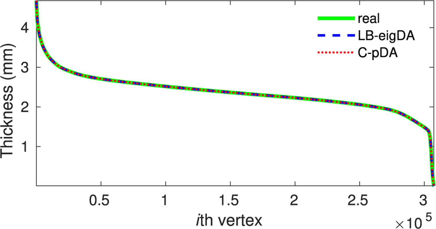
Sorted thickness values at each vertex on the cortical surface mesh. The green solid, blue dashed, and red dotted lines represent the thickness value at a particular vertex averaged over the 500 real samples, 500 augmented samples via LB-eigDA, and 500 augmented samples via C-pDA, respectively. For the purpose of visualization, the thickness averaged over 500 real samples is sorted in a descending manner across all the vertices on the cortical surface mesh. The average of augmented samples follows the sorted vertex index.

Fig. 11.

The distribution of the correlation between the 500 augmented thickness samples and the thickness averaged over 500 real samples (blue bar for the LB-eigDA and orange bar for the C-pDA method).

The LB-eigDA computational time was dependent on the number of the LB eigenfunctions, while the C-pDA computational time was related to the order of Chebyshev polynomials. Fig. 12 shows the LB-eigDA computational time as a function of the number of the LB eigenfunctions and the C-pDA computational time as the order of Chebyshev polynomials, K. The two augmentation methods were implemented in MATLAB (R2017b) using Intel Xeon Gold 5220S CPU (2.70 GHz). This figure suggests that more LB eigenfunctions used in LB-eigDA allow the augmentation over a wider spectrum but require a high computational cost when the cortical surface mesh is large (the cortical surface mesh with 327,684 vertices). The LB-eigDA computational cost was exponentially increased as the number of the LB eigenfunctions increased. In contrast, the C-pDA computational time was approximately a linear function of the order of Chebyshev polynomials. Compared to C-pDA, LB-eigDA was 70 times slower when K = 5000.

Fig. 12.

Computational time of the LB-eigDA (blue) and C-pDA (red-orange) methods for generating 500 augmented thickness samples from 500 randomly selected samples in the ADNI dataset.

4.3. Does classification improve by data augmentation?

We illustrate the use of the C-pDA method to classify healthy controls (HC) and AD patients based on the cortical thickness of the ADNI dataset. Again, we employed the LB-based spectral CNN with the architecture similar to that in Fig. 5, but used five convolutional layers. Each layer involved 8, 16, 32, 64, and 128 filters, respectively. The initial learning rate was 10⁻³, and the learning rate decay was 0.05 for every 20 epochs. In this experiment, the total number of samples from the ADNI dataset was 1709 (HC: n = 1122; AD: n = 587). Ten-fold cross-validation was adopted. One fold of real data was left out for testing. The remaining nine folds of data were further separated into training (75%) and validation (25%) sets. When the MRI dataset was separated into the training, validation, and testing sets, we considered subjects instead of MRI scans so that the scans from the same subjects were in the same set to avoid potential data over leakage.

The HC/AD classification accuracy based on the real ADNI data and the LB-based spectral CNN was 90.9 ± 0.6%. However, when only a smaller set of the real data was available (X% of the training set), that is, the training sample size was reduced, the classification accuracy dropped as illustrated by the red dashed line in Fig. 13. When only 10% of the real data was available, the classification accuracy was 75.8% and decreased 15% compared to that using the full ADNI data.

Fig. 13.

Classification accuracy. The red dashed line shows the classification accuracy when only X% of the real training samples were used in the training of the LB-based spectral CNN. The blue solid line shows the classification accuracy when only X% of the real raining set and 1 − X% of the augmented data were used in the training of the LB-based spectral CNN, where the augmented data were generated by the C-pDA method.

We previously showed that both C-pDA and LB-eigDA have the similar results but C-pDA was more computationally efficient than LB-eigDA. Thus, the following experiments only used C-pDA with 109 filters and the Chebyshev polynomials of order K = 5000. As illustrated in Fig. 6, the training samples contained X% of real ADNI data and 1 − X% augmented data, where X = 10, 20, …, 80. We added 1 − X% augmented data using C-pDA in the LB-based spectral CNN and computed the network performance using the testing real data. The augmentation was done separately for the HC and AD groups. For instance, when 90% of the training samples were augmented data and 10% of the training samples were real data, the classification accuracy was 83.3% and improved by 7.5%. Fig. 13 shows that C-pDA can increase the sample size and improve the HC/AD classification accuracy.

5. Discussion

This study introduces the LB-eigDA and C-pDA methods to generate augmented data on surfaces. Using the simulation with the ground truth label, we demonstrate that both methods improve the performance of graph-CNN. In particular, LB-eigDA has the potential to outperform C-pDA method since C-pDA approximates the LB spectral filters using Chebyshev polynomials. Nevertheless, when the mesh becomes large, LB-eigDA is computationally intensive while C-pDA is computationally efficient. C-pDA generates augmented thickness data and improves the AD classification accuracy in a real clinical application.

To our best knowledge, this study provides the first unbiased oversampling approaches for data augmentation on surfaces. These methods have a great potential to open new research areas in graph CNN in conjunction with generative adversarial networks (GANs). In particular, the formulation of the C-pDA method is consistent with that of the LB-based spectral CNN (Defferrard et al., 2016; Wee et al., 2019), which is feasible to adapt the C-pDA and graph network to the GAN framework. Further investigation will be needed.

References

- Apostolova LG, Dinov ID, Dutton RA, Hayashi KM, Toga AW, Cummings JL, et al. (2006). 3D comparison of hippocampal atrophy in amnestic mild cognitive impairment and Alzheimer’s disease. Brain, 129, 2867–2873. [DOI] [PubMed] [Google Scholar]
- Atwood J, & Towsley D (2015). Diffusion-convolutional neural networks. arXiv preprint arXiv:1511.02136. [Google Scholar]
- Basaia S, Agosta F, Wagner L, Canu E, Magnani G, Santangelo R, et al. (2019). Automated classification of Alzheimer’s disease and mild cognitive impairment using a single MRI and deep neural networks. NeuroImage: Clinical, 21, Article 101645. [DOI] [PMC free article] [PubMed] [Google Scholar]
- Bruna J, Zaremba W, Szlam A, & LeCun Y (2013). Spectral networks and locally connected networks on graphs. arXiv preprint arXiv:1312.6203. [Google Scholar]
- Chung MK, Qiu A, Seo S, & Vorperian HK (2015). Unified heat kernel regression for diffusion, kernel smoothing and wavelets on manifolds and its application to mandible growth modeling in CT images. Medical Image Analysis, 22, 63–76. [DOI] [PMC free article] [PubMed] [Google Scholar]
- Chung MK, & Taylor J (2004). Diffusion smoothing on brain surface via finite element method. In Proceedings of IEEE international symposium on biomedical imaging: Vol. 1, (pp. 432–435). [Google Scholar]
- Chung MK, Xie L, Huang S-G, Wang Y, Yan J, & Shen L (2019). Rapid acceleration of the permutation test via transpositions. In International workshop on connectomics in neuroimaging: Vol. 11848, (pp. 42–53). Springer. [DOI] [PMC free article] [PubMed] [Google Scholar]
- Coifman RR, & Maggioni M (2006). Diffusion wavelets. Applied and Computational Harmonic Analysis, 21, 53–94. [Google Scholar]
- Cuingnet R, Gerardin E, Tessieras J, Auzias G, Lehéricy S, Habert M-O, et al. (2011). Automatic classification of patients with Alzheimer’s disease from structural MRI: A comparison of ten methods using the ADNI database. NeuroImage, 56, 766–781. [DOI] [PubMed] [Google Scholar]
- Defferrard M, Bresson X, & Vandergheynst P (2016). Convolutional neural networks on graphs with fast localized spectral filtering. In Proceedings of the 30th international conference on neural information processing systems. (pp. 3844–3852). [Google Scholar]
- DeVries T, & Taylor GW (2017). Dataset augmentation in feature space. In 5th international conference on learning representations, Workshop track proceedings. OpenReview.net, URL https://openreview.net/forum?id=HyaF53XYx. [Google Scholar]
- Donnat C, Zitnik M, Hallac D, & Leskovec J (2018). Learning structural node embeddings via diffusion wavelets. In Proc. 24th ACM SIGKDD international conference on knowledge discovery & data mining (pp. 1320–1329). [Google Scholar]
- Du J, Younes L, & Qiu A (2011). Whole brain diffeomorphic metric mapping via integration of sulcal and gyral curves, cortical surfaces, and images. NeuroImage, 56, 162–173. [DOI] [PMC free article] [PubMed] [Google Scholar]
- Duvenaud DK, Maclaurin D, Aguilera-Iparraguirre J, Gomez-Bombarelli R, Hirzel T, Aspuru-Guzik A, et al. (2015). Convolutional networks on graphs for learning molecular fingerprints. arXiv preprint arXiv:1509.09292. [Google Scholar]
- Fan Y, Gur RE, Gur RC, Wu X, Shen D, Calkins ME, et al. (2008). Unaffected family members and schizophrenia patients share brain structure patterns: A high-dimensional pattern classification study. Biological Psychiatry, 63, 118–124. [DOI] [PMC free article] [PubMed] [Google Scholar]
- Fischl B, Salat DH, Busa E, Albert M, Dieterich M, Haselgrove C, et al. (2002). Whole brain segmentation: Automated labeling of neuroanatomical structures in the human brain. Neuron, 33, 341–355. [DOI] [PubMed] [Google Scholar]
- Ganin Y, Ustinova E, Ajakan H, Germain P, Larochelle H, Laviolette F, et al. (2016). Domain-adversarial training of neural networks. Journal of Machine Learning Research, 17, 1–35. [Google Scholar]
- Goodfellow I, Pouget-Abadie J, Mirza M, Xu B, Warde-Farley D, Ozair S, et al. (2014). Generative adversarial nets. In Advances in neural information processing systems (pp. 2672–2680). [Google Scholar]
- Goodfellow IJ, Shlens J, & Szegedy C (2014). Explaining and harnessing adversarial examples. arXiv preprint arXiv:1412.6572. [Google Scholar]
- Hammond DK, Vandergheynst P, & Gribonval R (2011). Wavelets on graphs via spectral graph theory. Applied and Computational Harmonic Analysis, 30, 129–150. [Google Scholar]
- Henaff M, Bruna J, & LeCun Y (2015). Deep convolutional networks on graph-structured data. arXiv preprint arXiv:1506.05163. [Google Scholar]
- Hosseini-Asl E, Keynton R, & El-Baz A (2016). Alzheimer’s disease diagnostics by adaptation of 3D convolutional network. In 2016 IEEE international conference on image processing (pp. 126–130). IEEE. [Google Scholar]
- Huang S-G, Lyu I, Qiu A, & Chung MK (2020). Fast polynomial approximation of heat kernel convolution on manifolds and its application to brain sulcal and gyral graph pattern analysis. IEEE Transactions on Medical Imaging, 39, 2201–2212. [DOI] [PMC free article] [PubMed] [Google Scholar]
- Hussain Z, Gimenez F, Yi D, & Rubin D (2017). Differential data augmentation techniques for medical imaging classification tasks. In Annual symposium proceedings (pp. 979–984). [PMC free article] [PubMed]
- Islam J, & Zhang Y (2018). Brain MRI analysis for Alzheimer’s disease diagnosis using an ensemble system of deep convolutional neural networks. Brain Informatics, 5, 2. [DOI] [PMC free article] [PubMed] [Google Scholar]
- James G, Witten D, Hastie T, & Tibshirani R (2013). An introduction to statistical learning. volume 112. Springer. [Google Scholar]
- Ker J, Wang L, Rao J, & Lim T (2017). Deep learning applications in medical image analysis. IEEE Access, 6, 9375–9389. [Google Scholar]
- Kim WH, Pachauri D, Hatt C, Chung MK, Johnson S, & Singh V (2012). Wavelet based multi-scale shape features on arbitrary surfaces for cortical thickness discrimination. In Advances in neural information processing systems (pp. 1241–1249). [PMC free article] [PubMed] [Google Scholar]
- Kingma DP, & Welling M (2013). Auto-encoding variational Bayes. arXiv preprint arXiv:1312.6114. [Google Scholar]
- Kipf TN, & Welling M (2016). Semi-supervised classification with graph convolutional networks. arXiv preprint arXiv:1609.02907. [Google Scholar]
- Korolev S, Safiullin A, Belyaev M, & Dodonova Y (2017). Residual and plain convolutional neural networks for 3D brain MRI classification. In 2017 IEEE 14th international symposium on biomedical imaging (pp. 835–838). IEEE. [Google Scholar]
- Ktena SI, Parisot S, Ferrante E, Rajchl M, Lee M, Glocker B, et al. (2017). Distance metric learning using graph convolutional networks: application to functional brain networks. arXiv preprint arXiv:1703.02161. [Google Scholar]
- Leevy JL, Khoshgoftaar TM, Bauder RA, & Seliya N (2018). A survey on addressing high-class imbalance in big data. Journal of Big Data, 5, 42. [Google Scholar]
- Li Y, Tarlow D, Brockschmidt M, & Zemel R (2015). Gated graph sequence neural networks. arXiv preprint arXiv:1511.05493. [Google Scholar]
- Litjens G, Kooi T, Bejnordi BE, Setio AAA, Ciompi F, Ghafoorian M, et al. (2017). A survey on deep learning in medical image analysis. Medical Image Analysis, 42, 60–88. [DOI] [PubMed] [Google Scholar]
- Liu X, Tosun D, Weiner MW, Schuff N, Alzheimer’s Disease Neuroimaging Initiative, et al. (2013). Locally linear embedding (LLE) for MRI based Alzheimer’s disease classification. NeuroImage, 83, 148–157. [DOI] [PMC free article] [PubMed] [Google Scholar]
- Liu M, Zhang J, Adeli E, & Shen D (2018). Landmark-based deep multi-instance learning for brain disease diagnosis. Medical Image Analysis, 43, 157–168. [DOI] [PMC free article] [PubMed] [Google Scholar]
- Mazurowski MA, Habas PA, Zurada JM, Lo JY, Baker JA, & Tourassi GD (2008). Training neural network classifiers for medical decision making: The effects of imbalanced datasets on classification performance. Neural Networks, 21, 427–436. [DOI] [PMC free article] [PubMed] [Google Scholar]
- Meyer M, Desbrun M, Schröder P, & Barr AH (2003). Discrete differential-geometry operators for triangulated 2-manifolds. In Visualization and mathematics III (pp. 35–57). Springer. [Google Scholar]
- Niepert M, Ahmed M, & Kutzkov K (2016). Learning convolutional neural networks for graphs. In Proceeding of the 33rd international conference on machine learning (pp. 2014–2023). ACM. [Google Scholar]
- Oppenheim AV, Schafer RW, & Buck JR (1999). Discrete-time signal processing. Upper Saddle River, NJ: Prentice Hall. [Google Scholar]
- Perozzi B, Al-Rfou R, & Skiena S (2014). Deepwalk: Online learning of social representations. In Proceedings of the 20th ACM SIGKDD (pp. 701–710). ACM. [Google Scholar]
- Qiu A, Bitouk D, & Miller MI (2006). Smooth functional and structural maps on the neocortex via orthonormal bases of the Laplace-Beltrami operator. IEEE Transactions on Medical Imaging, 25, 1296–1396. [DOI] [PubMed] [Google Scholar]
- Qiu A, Fennema-Notestine C, Dale AM, Miller MI, & the Alzheimer’s Disease Neuroimaging Initiative (2009). Regional shape abnormalities in mild cognitive impairment and Alzheimer’s disease. NeuroImage, 45, 656–661. [DOI] [PMC free article] [PubMed] [Google Scholar]
- Ranginwala NA, Hynan LS, Weiner MF, & White CL III (2008). Clinical criteria for the diagnosis of Alzheimer disease: Still good after all these years. American Journal of Geriatric Psychiatry, 16, 384–388. [DOI] [PubMed] [Google Scholar]
- Ravanbakhsh S, Schneider J, & Poczos B (2016). Deep learning with sets and point clouds. arXiv preprint arXiv:1611.04500. [Google Scholar]
- Shen D, Wu G, & Suk H-I (2017). Deep learning in medical image analysis. Annual Review of Biomedical Engineering, 19, 221–248. [DOI] [PMC free article] [PubMed] [Google Scholar]
- Shorten C, & Khoshgoftaar TM (2019). A survey on image data augmentation for deep learning. Journal of Big Data, 6, 60. [DOI] [PMC free article] [PubMed] [Google Scholar]
- Shuman DI, Ricaud B, & Vandergheynst P (2016). Vertex-frequency analysis on graphs. Applied and Computational Harmonic Analysis, 40, 260–291. [Google Scholar]
- Tan M, & Qiu A (2015). Spectral Laplace-Beltrami wavelets with applications in medical images. IEEE Transactions on Medical Imaging, 34, 1005–1017. [DOI] [PubMed] [Google Scholar]
- Tang Y (2013). Deep learning using linear support vector machines. arXiv preprint arXiv:1306.0239. [Google Scholar]
- Tong T, Wolz R, Gao Q, Guerrero R, Hajnal JV, Rueckert D, et al. (2014). Multiple instance learning for classification of dementia in brain MRI. Medical Image Analysis, 18, 808–818. [DOI] [PubMed] [Google Scholar]
- Wang Y, Ombao H, & Chung MK (2018). Topological data analysis of single-trial electroencephalographic signals. Annals of Applied Statistics, 12, 1506–1534. [DOI] [PMC free article] [PubMed] [Google Scholar]
- Wee C-Y, Liu C, Lee A, Poh JS, Ji H, Qiu A, et al. (2019). Cortical graph neural network for AD and MCI diagnosis and transfer learning across populations. NeuroImage: Clinical, 23, Article 101929. [DOI] [PMC free article] [PubMed] [Google Scholar]
- Yang X, Goh A, Chen SH, & Qiu A (2013). Evolution of hippocampal shapes across the human lifespan. Human Brain Mapping, 34, 3075–3085. [DOI] [PMC free article] [PubMed] [Google Scholar]
- Yi L, Su H, Guo X, & Guibas L (2017). SyncSpecCNN: Synchronized spectral CNN for 3D shape segmentation. In Computer vision and pattern recognition, conference on (pp. 6584–6592). IEEE. [Google Scholar]
- Yi X, Walia E, & Babyn P (2019). Generative adversarial network in medical imaging: A review. Medical Image Analysis, 58, Article 101552. [DOI] [PubMed] [Google Scholar]
- Zhong J, Phua DYL, & Qiu A (2010). Quantitative evaluation of LDDMM, FreeSurfer, and CARET for cortical surface mapping. NeuroImage, 52, 131–141. [DOI] [PubMed] [Google Scholar]
- Zhong Z, Zheng L, Kang G, Li S, & Yang Y (2017). Random erasing data augmentation. ArXiv Preprint arXiv:1708.04896. [Google Scholar]