Improving estimates of Medicaid's effect on poverty: Measures and counterfactuals

Abstract

Objective

To re‐evaluate the effect of Medicaid on poverty using a poverty measure that accounts for health insurance needs and benefits and an evaluation approach that reflects disparities in access to alternative coverage.

Data Sources

The Current Population Survey (CPS) for calendar year 2015.

Study Design

We estimate the effect of losing Medicaid on poverty, combining two previous approaches: (1) A propensity impact, which simulates a no‐Medicaid counterfactual incorporating changes to health insurance and medical out‐of‐pocket spending, using the Supplemental Poverty Measure (SPM). This measure does not reflect a need for health care access nor how health benefits meet that need. (2) An accounting impact, which assumes that those losing Medicaid remain uninsured and does not incorporate any behavioral changes, using the health‐inclusive poverty measure (HIPM). This measure includes a need for health insurance in the threshold and health insurance benefits in resources.

Data Collection/Extraction Methods

Not applicable.

Principal Findings

Using the propensity‐matched approach, we attributed a 2.5 percentage point reduction in health‐inclusive poverty among those younger than age 65 to the Medicaid program, between the 1.0‐point SPM propensity‐match impact and the 3.9‐point HIPM accounting impact. Medicaid's antipoverty impact and HIPM‐SPM differences are greater among those who would become uninsured. HIPM propensity‐matched estimates reveal much larger impacts of Medicaid on poverty disparities linked to race/ethnicity and single parenthood than SPM‐based propensity estimates.

Conclusions

Both the poverty measure and the method used to estimate the counterfactual make substantial, policy‐relevant differences to estimates of Medicaid's impact on poverty. A poverty measure that fails to incorporate health insurance needs and benefits substantially underestimates Medicaid's effect. Failing to consider adjustments in insurance coverage and out‐of‐pocket spending substantially overestimates Medicaid's effect and underestimates its reduction of disparities.

What is known on this topic

• Uninsured households frequently delay or forgo needed care.

• If health care coverage is considered a need, then households who have no health benefits and cannot afford to purchase health insurance will be considered impoverished according to the health‐inclusive poverty measure.

• Medicaid reduces poverty by providing access to needed health care coverage and by limiting out‐of‐pocket expenses.

What this study adds

• This study combines the health‐inclusive poverty measure, which incorporates health insurance needs and benefits in poverty measurement, with a propensity‐match technique for evaluating the Medicaid's impact on poverty, a technique previously only applied to the non‐health‐inclusive Supplemental Poverty Measure (SPM).

• This study's estimates of Medicaid's impact on poverty fall between the smaller SPM estimate, which does not incorporate insurance needs or benefits, and the larger accounting estimate, which does not incorporate access to alternative coverage when evaluating health‐inclusive poverty.

• The combined approach illustrates the importance of evaluating access to substitute coverage in estimating health‐inclusive poverty effects, by highlighting disparities in access to substitute coverage that would be observed in the absence of the Medicaid program, both racially and for single‐adult households with children.

1. INTRODUCTION

Medicaid expansion improved the health and economic well‐being of its low‐income beneficiaries. Studies find evidence of increased health care utilization, reduced mortality, reduced home evictions, and many other benefits. ¹ , ² , ³ , ⁴ , ⁵ , ⁶ However, the extent to which Medicaid reduces poverty remains unsettled because different estimates have different shortcomings.

Sommers and Oellerich ⁷ and, more recently, Zewde and Wimer ⁸ have estimated the antipoverty impact of Medicaid using the Supplemental Poverty Measure (SPM). ⁹ Researchers increasingly use the SPM to evaluate the poverty effects of policy, partly because, unlike the official poverty measure, it incorporates most in‐kind benefits. For example, a National Academy of Sciences panel on reducing child poverty was mandated to use the SPM for its analyses. ¹⁰ However, that panel recommended US statistical agencies evaluate the health‐inclusive poverty measure (HIPM) ¹¹ for assessing health insurance programs, such as Medicaid (recommendation 9‐1) ¹⁰ because it, unlike the SPM, explicitly incorporates health needs and benefits. A government report on improving poverty measure supported that goal (see Recommendations 4, 5, and 13). ¹² While both the SPM and the HIPM capture Medicaid's antipoverty effects through reductions to out‐of‐pocket (OOP) medical spending, the HIPM alone captures how Medicaid reduces unmet health care needs. The distinction can be critical. Many low‐income Medicaid beneficiaries would become uninsured in the absence of public coverage, face high prices for medical care, forgo some medical needs, and spend little OOP on health care, yet barely register any increase in SPM poverty.

To date, estimates of Medicaid's impact on HIPM poverty have not directly incorporated how those losing Medicaid might gain substitute insurance. ¹³ , ¹⁴ Most use the accounting approach. One uses cross‐sectional data to estimate regression‐adjusted impacts of Medicaid expansion on HIPM poverty. ¹⁵ But none is able to shed light on the importance of counterfactual coverage driving health‐inclusive poverty and disparities in health‐inclusive poverty. This shortcoming matters because insurance benefits are a main determinant of HIPM poverty. In this paper, we estimate the impact of Medicaid on health‐inclusive poverty using a more rigorous propensity‐match technique previously applied only to the SPM. We examine the empirical implications of both poverty measures and counterfactual approaches and how they interact.

1.1. Poverty measures: Supplemental and health inclusive

Poverty is generally defined as the inability to meet one's basic needs. While simple in theory, the construct of “needs” remains incompletely defined, especially with respect to health care and insurance. The Census Bureau's SPM defines a household's needs as, essentially, resources sufficient to purchase an adequate level of food, clothing, shelter, and utilities—nonhealth needs. ¹⁶ To address health care and insurance, the SPM deducts from income all OOP spending on medical care, health insurance, and over‐the‐counter medications. SPM poverty status is determined by whether after‐deduction income is sufficient to meet nonhealth needs. Someone without coverage who foregoes and does not pay for essential medical care is implicitly deemed to have no basic need for such care. Difference‐in‐difference studies of the effects of Medicaid expansions or the Medicaid program on poverty have used the SPM measure of poverty ⁷ , ⁸ and are therefore unable to show Medicaid's direct impact on poverty—how it helps meet the need for health care coverage. ¹¹

In contrast, the HIPM includes health care coverage among the basic needs and shows how health benefits can meet that need. Specifically, the HIPM defines poverty as the inability to meet the need for health insurance coverage in addition to food, clothing, shelter, and utilities. The HIPM includes health insurance benefits, whether employer‐ or government‐provided, in the family's resources available to meet health needs. Therefore, the HIPM can show how Medicaid reduces poverty directly, meeting households' need for health care by providing full coverage. ^{10 (Ch7,9), 11} , ¹³ , ¹⁴ The HIPM has been used to quantify the direct impact of Medicaid, Medicare, and ACA premium subsidies on poverty. ¹¹ , ¹³ , ¹⁴

1.2. Estimation of change in poverty: Accounting and propensity‐matched

Studies of the extent to which Medicaid reduces health‐inclusive poverty have not used rigorous approaches to estimate the no‐Medicaid counterfactual. Prior HIPM studies mostly use the “accounting” approach (the same method used to estimate the impact of nonhealth benefits in Census poverty reports ¹⁶ ), which sets the value of Medicaid benefits to zero. ¹³ , ¹⁴ , ¹⁷

The HIPM accounting approach (a‐HIPM) is partly consistent with evidence suggesting that, without Medicaid, many recipients would be unable to secure alternative health care benefits. Nevertheless, some recipients would gain alternative coverage. Moreover, some who would become uninsured or receive alternative care would spend more OOP on health care. HIPM accounting studies capture neither effect. HIPM poverty rates could be quite sensitive to alternative coverage because health insurance and care expenditures can be large.

Studies using the SPM have incorporated compelling OOP spending counterfactuals through a propensity‐score matching approach ⁷ , ⁸ to simulate a counterfactual world without Medicaid. Counterfactual OOP spending on care and insurance are combined with other baseline characteristics to calculate a counterfactual SPM poverty status. The antipoverty impact of Medicaid is the difference in SPM poverty rates between that counterfactual and the baseline. The approach matches Medicaid beneficiaries to otherwise similar individuals without Medicaid coverage and assumes the beneficiary would incur their level of OOP spending if Medicaid were suddenly eliminated. This propensity‐match SPM approach (p‐SPM) captures the poverty impacts of potential increases in OOP spending that individuals losing Medicaid coverage might incur. Still, this approach cannot reflect the value of lost medical benefits, since the SPM captures the poverty effects of health care only through changes in OOP spending. Many Medicaid beneficiaries would become uninsured in the absence of Medicaid, as many were prior to their enrolment. ¹⁸ Because most uninsured, low‐income individuals spend very little on care, the inability of the newly uninsured to meet their basic needs would barely register in a measure that captures only changes to OOP spending.

Applying the match approach to the HIPM, by contrast, could illustrate both the changes to OOP spending and the loss of health care benefits, by using counterfactual insurance status. This propensity‐match HIPM (p‐HIPM) is particularly valuable in evaluating disparities that stem from differential access to substitute health insurance benefits. Such disparities occur for several reasons. Those with strong ties to the labor force have better access to employer‐sponsored insurance. Pregnant women and mothers of small children are currently eligible for Medicaid at higher levels of income than nonparents. Higher‐income beneficiaries may be better able to transition to private insurance through their own or a spouse's employment‐based policy. Likewise, when coverage is more contingent on employment, black Americans and other minorities may have less access to health care though an employer either because of lower employment rates or because their employers and industries of employment are less likely to offer health insurance benefits. ¹⁹ Finally, nonelderly individuals with work‐limiting disabilities may be less likely to have private insurance benefits in the absence of Medicaid and may not meet disability requirements for Medicare coverage. Neither the accounting approach applied to the HIPM nor the p‐SPM can evaluate Medicaid's role in reducing disparate access to private health care benefits that may be observed in the program's absence.

The two prior approaches to estimating Medicaid's antipoverty impact likely provide upper and lower bounds to the true impact. The SPM‐propensity score matching studies found that between 0.9% and 1.4% of the US population avoids poverty annually due to Medicaid coverage. ⁷ , ⁸ This is likely a lower bound because the loss of Medicaid affects SPM poverty only through an increase in OOP spending not through unmet health care needs. The HIPM‐accounting studies find an impact estimate of 3.8% points for the population younger than age 65. ¹³ , ¹⁴ This is likely an upper bound because it does not recognize the availability of substitute coverage among those who would lose Medicaid.

This paper integrates these two approaches, computing the HIPM using propensity‐matching approach, improving estimates Medicaid's antipoverty impact and poverty disparities by race, Hispanic ethnicity, and family structure. This analysis also illustrates how the counterfactual approach and poverty measure interact to affect those estimates. Statistical agencies that evaluate the HIPM will need to understand the importance of counterfactual methods for HIPM estimates. Moreover, this work will help inform state policy makers of the consequences of Medicaid disenrollment, or conversely of expanding Medicaid, on the poverty rates of implicated households. Once we account for any alternative coverage source in its absence, to what extent does Medicaid reduce health‐inclusive poverty and reduce poverty disparities?

2. METHODS

2.1. Sample

We analyze data from the Current Population Survey's Annual Social and Economic Supplement, conducted in March 2016, covering a representative sample of the population for the year 2015. Data on households' income, benefits, and SPM thresholds come from the Census Bureau's SPM research file. We apply CPS March Supplement weights to produce estimates representative of the US population and use replicate weights to calculate confidence intervals and sampling errors accounting for the survey's complex sampling design.

We calculate poverty rates for the population, measured as the share of individuals whose household's resources are less than the household's needs threshold. SPM threshold and resources are fully described in Short (2011), and HIPM threshold and resources are fully described in the Appendix to Remler et al. (2017). We use the SPM family unit (or “resource unit”), which includes unmarried cohabiters, among others. We present poverty rates only for individuals who are younger than age 65 (N = 161,513). However, since those individuals may reside with persons older than age 65, we retain all observations to evaluate household‐level variables.

For the HIPM, we gathered additional health insurance premium, cost sharing, and program eligibility information from three sources: ACA Marketplace plans ²⁰ ; Medicare Advantage Prescription Drug Plans ²¹ ; and premium and cost‐sharing rules for Medicaid and the Children's Health Insurance Program. ²² To determine eligibility for means‐tested ACA premium subsidies and reduced cost‐sharing caps, we used the family health insurance units defined in the IPUMS‐CPS data. ²³ We imputed undocumented status and, therefore, ineligibility for ACA premium subsides using Borjas's method. ²⁴

2.2. Supplemental and health‐inclusive poverty measures

A household is deemed poor according to the SPM if household resources—cash income, net of taxes, tax credits, and means‐tested nonhealth benefits—exceed a threshold level of needs for food, clothing, shelter, and utilities ²⁵ but not for health insurance or health care. The SPM incorporates an implicit need for OOP spending on health insurance and health care by deducting from resources all medical out‐of‐pocket (MOOP) spending on care (nonpremium MOOP) and insurance (premium MOOP). The SPM could not treat health insurance benefits like cash resources, as it does for food or housing assistance, unless the needs threshold included health insurance or health care. Doing so would imply health benefits could meet food or housing needs. ²⁶ The inconsistent and highly concentrated nature of health care needs makes health insurance benefits largely not fungible. ^{14 (pp6‐7)}

The HIPM adds to the SPM needs threshold an explicit need for basic health insurance. For most of the population younger than age 65, the dollar value of the health insurance need is the premium of the benchmark (second‐lowest cost) Silver plan available on the ACA Marketplace. For Medicare recipients, the health insurance need is the full cost (government and beneficiary contributions) of the lowest cost Medicare‐Advantage plan (bundled with prescription drug coverage) available in the county of residence.

Next, for those with public or private health benefits, the HIPM adds to SPM resources a value for those benefits. The HIPM treats those with and without health benefits very differently. Those with employer‐ or government‐provided health benefits have their health need fully met. Those without benefits (the uninsured and those who purchase their own insurance) will be designated poor unless they have income sufficient to purchase health insurance and meet nonhealth needs. Those with nongroup insurance are credited with income‐based ACA subsidies as resources, if eligible. HIPM and SPM poverty status differ sharply for those who are uninsured or who purchase their own insurance, who need enough income to purchase health insurance in order to not be HIPM poor.

Like the SPM, the HIPM includes a nonpremium MOOP subtraction, though it limits that subtraction to an OOP maximum that depends on insurance type. We summarize differences between the SPM and HIPM, as well as the official poverty measure in Figure A1. Detailed information on the modifications and cost‐sharing specifications in the HIPM is provided in the following. ¹¹ , ¹³ , ¹⁴

2.3. Counterfactuals and estimated poverty impacts

Simulating the impact of Medicaid on poverty requires calculating a poverty rate under both baseline (status quo with the Medicaid program) and counterfactual (without the Medicaid program) conditions and taking the difference. We define Medicaid coverage at baseline as individuals reporting at least 1 month of Medicaid coverage during the year; we do not distinguish between Medicaid and the Children's Health Insurance Program. We take two approaches to the counterfactual. First, we use the accounting approach used in prior studies and, for nonhealth benefits, in Census Bureau's poverty reports. ¹⁶ This approach simply removes the value of Medicaid benefits, without estimating the change in OOP spending or crediting the value of ACA premium subsidies, employer‐provided health insurance, or Medicare that the household might obtain if they lost Medicaid. The household becomes HIPM poor in the accounting counterfactual if they lack the income to pay for a standard ACA policy in addition to paying for the nonhealth components of the poverty threshold. ¹¹ , ¹⁴ It is not possible to estimate an SPM accounting approach for Medicaid impact because the SPM does not include health benefits in resources.

For the propensity‐match approach, we aim to predict the source of coverage (if any) and level of OOP spending on care and insurance that an individual with Medicaid would incur if their Medicaid coverage was eliminated. Then, we use individuals' baseline characteristics (like income) along with their counterfactual MOOP and insurance to calculate counterfactual poverty. ⁷ , ⁸

To implement the propensity‐match approach, we first predict individuals' propensity to have Medicaid coverage, through logistic regressions, stratified across five groups defined by the individual's pathway to Medicaid eligibility (children aged 0–18, nonelderly adults with disabilities, nonelderly parents of dependent children, other nonelderly adults, and adults age 65 and older). Covariates are mostly the same across the strata with some commonsense differences (e.g., models for children exclude marital status and full‐time work covariates). Covariates include socioeconomic indicators (household income, presence of interest or dividend income in the household, and individuals' level of education, employment status and student status), demographic indicators (20 age‐by‐gender categories, marital status, race, citizenship status, and household size), five self‐reported health categories, and an indicator for Medicaid eligibility, which we impute based on state eligibility rules for households in each eligibility category, and state‐fixed effects. For full models, see Tables A1 and A2.

Next, we randomly match individuals with Medicaid coverage to non‐Medicaid individuals within the same decile of the estimated propensity score, ⁷ , ²⁷ stratified by five eligibility groups, creating 50 imputation cells. We sample nonbeneficiaries with replacement.

We assign beneficiaries their matched counterpart's health insurance status and OOP expenditures on insurance and care. However, beneficiaries do not take on other counterfactual characteristics, such as income, family structure, employment status, residential location, or other public benefits receipt not directly affected by the removal of Medicaid. We assume that insurance coverage and any OOP spending on care or premiums are the only components of household income directly affected by the elimination of Medicaid. We do not model effects on labor supply, as this relationship lacks evidence, nor on benefit take‐up, which has empirically shown modest responses in prior studies. For example, evidence from the Oregon Health Insurance Experiment shows no change in labor market activity nor in the value of cash assistance received and an approximately 7% increase in the value of food stamps (from a base of $1000) associated with Medicaid eligibility. ²⁸ , ²⁹ Eligibility for premium subsidies and amounts of these subsidies in the counterfactual are determined by the household's baseline cash income. See Tables A3–A7 for comparability of imputation cells on key matching variables.

2.4. Matching counterfactual sensitivity analysis

While, in the absence of Medicaid, beneficiaries might obtain employer coverage or purchase individual coverage, we expect the share doing so to be small. ACA Medicaid expansion studies suggest that there was little crowd‐out of employer‐provided insurance, and some studies find close to one‐for‐one substitution between un‐insurance and Medicaid. ² Prior counterfactual matching estimates, which used the SPM to measure poverty, imply that a substantial share (46.5%) of those losing Medicaid would gain private insurance, which may be overly optimistic. ⁷

We therefore performed a sensitivity analysis, restricting the counterfactual health insurance outcomes to either uninsured or Medicare. Specifically, we removed individuals with private insurance (employer or individual purchase) from the pool of potential matches. This left 37,551 potential matches (down from 154,069 in the unrestricted approach) for 31,411 Medicaid beneficiaries in the sample. We then estimated revised p‐HIPM and p‐SPM impacts using the same methods. Because Medicaid loss affects SPM poverty only through reductions in MOOP, we expect the restricted analysis to show a larger impact for the p‐HIPM and little, if any, for the p‐SPM.

3. RESULTS

3.1. Propensity score‐matching HIPM estimates

Combining the propensity‐matching approach with the health‐inclusive measure, we estimate that Medicaid reduces poverty by 2.5 percentage points (Figure 1, for the US population younger than age 65). This preferred estimate lies essentially midway between the estimates from the SPM propensity‐matching approach (1.0 percentage point) and a‐HIPM (3.9 percentage points).

FIGURE 1.

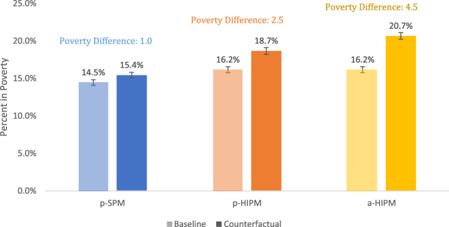
Rates of poverty with and without Medicaid by evaluation approach and poverty measure. This figure presents estimates of the US poverty rates at baseline and in a counterfactual scenario without Medicaid using data from the 2016 Current Population Survey' Annual Social and Economic Supplement. Counterfactual scenarios simulated with a propensity‐matched technique described in the text. Poverty impacts evaluated with the Supplemental Poverty Measure (p‐SPM) and Health Inclusive Poverty Measure (p‐HIPM). The accounting approach (a‐HIPM) assumes all beneficiaries become uninsured in the absence of Medicaid. Due to rounding, poverty difference may not exactly equal difference between baseline and counterfactual rates shown. Confidence intervals are calculated using CPS replicate weights to account for complex sampling design [Color figure can be viewed at wileyonlinelibrary.com]

According to our preferred p‐HIPM estimate, in the absence of Medicaid coverage, beneficiaries who become uninsured realize the greatest increase in poverty, 6.6 percentage points, approximately 65% greater than the 4.0 percentage point increase observed for those who obtain nongroup coverage and (potentially) ACA premium subsidies (Figure 2). By contrast, the p‐SPM estimate suggests only a small difference in Medicaid impacts between these groups (a 1.9 percentage point for the newly uninsured and 1.6 points for the nongroup insured). Comparing the two, we find the smallest difference between the p‐HIPM and p‐SPM impacts among those who transition to employer‐sponsored coverage: an HIPM impact of 1.4 versus an SPM impact of 0.7 percentage points (Figure 2).

FIGURE 2.

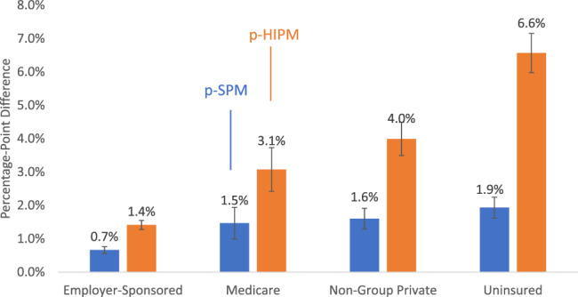
Medicaid's antipoverty impact, by counterfactual coverage, measured by SPM and HIPM. This figure presents estimates of the change in poverty rates between the baseline scenario and a counterfactual scenario without Medicaid using data from the 2016 Current Population Survey's Annual Social and Economic Supplement. Estimates are presented by counterfactual insurance status, which groups together both those who had that insurance status at baseline and those who obtained it in the counterfactual after losing Medicaid. Counterfactual scenarios simulated with a propensity‐matched technique described in the text. Poverty impacts evaluated with the Supplemental Poverty Measure (p‐SPM) and Health Inclusive Poverty Measure (p‐HIPM). Due to rounding, poverty difference may not exactly equal difference between baseline and counterfactual rates shown. Confidence intervals are calculated using CPS replicate weights to account for complex sampling design [Color figure can be viewed at wileyonlinelibrary.com]

3.2. Demographic variation

Differences across races in the poverty impact of Medicaid coverage are larger according to the p‐HIPM than the p‐SPM (Figure 3). When Medicaid is eliminated, 4.1% of blacks and 4.9% of Hispanics fall into HIPM poverty, compared to 1.4% of whites. Thus, Medicaid reduces racial/ethnic gaps in HIPM poverty by 2.7–3.5 percentage points. In contrast, the SPM results suggest that Medicaid reduces racial disparities in poverty by only about 1 percentage point (Figure 3).

FIGURE 3.

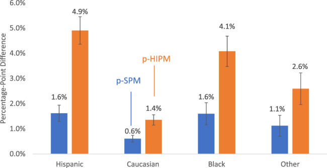
Medicaid's antipoverty impact by race and ethnicity, measured by SPM and HIPM. This figure presents estimates of the change in poverty rates between the baseline scenario and a counterfactual scenario without Medicaid using data from the 2016 Current Population Survey's Annual Social and Economic Supplement. Estimates are presented by Hispanic ethnicity and racial identification. Counterfactual scenarios simulated with a propensity‐matched technique described in the text. Poverty impacts evaluated with the Supplemental Poverty Measure (p‐SPM) and Health Inclusive Poverty Measure (p‐HIPM). Due to rounding, poverty difference may not exactly equal difference between baseline and counterfactual rates shown. Confidence intervals are calculated using CPS replicate weights to account for complex sampling design [Color figure can be viewed at wileyonlinelibrary.com]

Additionally, the p‐HIPM shows a higher Medicaid impact for single parents, relative to other family structures (Figure 4). With either the p‐SPM or p‐HIPM, twice as many single‐parent families fall into poverty without Medicaid than do married or nonparent families. Still, HIPM poverty rates are higher than SPM rates, which implies larger absolute differences in Medicaid impacts. According to the HIPM, Medicaid reduces the poverty rate of single parents by more than 5 percentage points versus 1.9 percentage points among married parents and 2.5 percentage points for nonparents. For the SPM, single parents experience a relatively modest 2.1 percentage point increase in poverty, while the impact on married parents and nonparents is under 1 percentage point.

FIGURE 4.

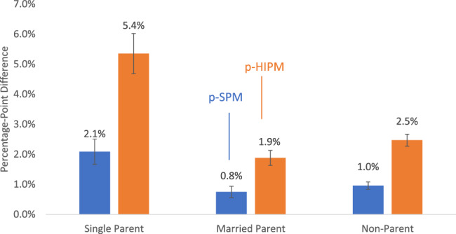
Medicaid's antipoverty impact by household structure, measured by HIPM and SPM. This figure presents estimates of the change in poverty rates between the baseline scenario and a counterfactual scenario without Medicaid using data from the 2016 Current Population Survey's Annual Social and Economic Supplement. Estimates are presented by household structure. Counterfactual scenarios simulated with a propensity‐matched technique described in the text. Poverty impacts evaluated with the Supplemental Poverty Measure (p‐SPM) and Health Inclusive Poverty Measure (p‐HIPM). Due to rounding, poverty difference may not exactly equal difference between baseline and counterfactual rates shown. Confidence intervals are calculated using CPS replicate weights to account for complex sampling design [Color figure can be viewed at wileyonlinelibrary.com]

3.3. Sensitivity analysis

Our sensitivity analyses restrict counterfactual Medicaid coverage type for those who lose Medicaid to either un‐insurance or Medicare, 96% and 4%, respectively. The estimated impact on HIPM poverty increases to 4.2 percentage points, compared to 2.5 percentage points in the unrestricted counterfactual match (Table 1). By contrast, the restricted match reduces the estimated impact on SPM poverty to 0.3 percentage point, compared to a 1.0‐point change with the unrestricted counterfactual. This SPM estimate aligns with the sensitivity tests reported in the existing literature. ^{7 (p825)}

TABLE 1.

Antipoverty impacts of Medicaid using unrestricted and restricted match criteria, by demographic groups

	Unrestricted match		No private insurance, match to uninsured or Medicare
	p‐SPM	p‐HIPM	p‐SPM	p‐HIPM
Total population	1.0 (0.06)	2.5 (0.10)	0.3 (0.05)	4.2 (0.12)
By parenthood
No children	1.0 (0.06)	2.5 (0.10)	0.3 (0.05)	4.1 (0.12)
Parent	1.0 (0.09)	2.6 (0.12)	0.3 (0.06)	4.5 (0.14)
By family structure
Single parent	2.1 (0.21)	5.4 (0.34)	0.9 (0.17)	8.7 (0.40)
Married parent	0.8 (0.10)	1.9 (0.13)	0.1 (0.07)	3.3 (0.16)
Nonparent	1.0 (0.06)	2.5 (0.10)	0.3 (0.05)	4.1 (0.12)
By age
0–18	1.4 (0.12)	3.8 (0.19)	0.5 (0.09)	6.3 (0.21)
19–54	0.9 (0.06)	2.0 (0.09)	0.3 (0.04)	3.4 (0.11)
55–64	0.7 (0.09)	1.9 (0.13)	0.2 (0.07)	3.1 (0.17)
By race/ethnicity
Hispanic	1.6 (0.16)	4.9 (0.28)	0.4 (0.11)	8.0 (0.30)
White	0.6 (0.07)	1.4 (0.10)	0.2 (0.05)	2.4 (0.12)
Black	1.6 (0.22)	4.1 (0.31)	0.6 (0.18)	6.6 (0.43)
Other	1.1 (0.21)	2.6 (0.32)	0.5 (0.19)	4.0 (0.39)

Note: Table presents estimates of the change in poverty between baseline and two specifications of a counterfactual scenario without Medicaid, each using data from the 2016 Current Population Survey's Annual Social and Economic Supplement. “Unrestricted match” matches Medicaid beneficiaries to any otherwise‐similar nonbeneficiary. “No Private Insurance” restricts the pool of potential matches to those who are either uninsured or who have Medicare but have no private insurance. Match approaches applied to the Health‐inclusive Poverty Measure (p‐HIPM) and the Supplemental Poverty Measure (p‐SPM). Standard Errors (SE) shown in parentheses. Due to rounding, poverty difference may not exactly equal difference in baseline and counterfactual rates shown. SEs calculated using CPS replicate weights for complex sampling design.

The restricted match estimates show qualitatively similar but larger differences between the poverty measures in the impact of Medicaid on demographic gaps in poverty (Table 1). Tellingly, among individuals between the ages of 55 and 64 who lose Medicaid and become uninsured, only two‐tenths of a percentage point become unable to meet basic needs using the SPM definition, as compared with 3.1 percentage points using the HIPM definition, more than 15 times as many (Table 1).

4. DISCUSSION AND CONCLUSIONS

We attribute a 2.5 percentage point reduction in health‐inclusive poverty to the Medicaid program, using the propensity‐matched HIPM to account for substitution to available coverage alternatives. This estimate is 0.8 points larger than the 1.7 point regression‐adjusted difference in health‐inclusive poverty between Medicaid expansion and nonexpansion state reported elsewhere. ¹⁵ The difference could be due either to weaker controls in prior, cross‐sectional analysis or because the Medicaid overall has a bigger effect than Medicaid expansion alone. Our preferred estimate is also 1.4 points smaller than our accounting HIPM estimate of 3.9 points, which is comparable to the 3.8‐point estimate in the literature. ¹³

Our estimated Medicaid impact on SPM poverty is 1.0 percentage points, less than half the estimated impact on HIPM poverty. Our SPM poverty result is comparable to prior propensity‐matched SPM estimates of between 0.9 and 1.4 points, although those studies included adults older than 65 years. ⁷ , ⁸ Thus, accounting for health insurance needs and benefits, in addition to OOP medical and insurance expenses, more than doubles Medicaid's impact on poverty.

The discrepancy between the poverty measures in Medicaid impacts is particularly large for those who become uninsured without Medicaid. The effect on SPM poverty is very small for this group because the uninsured tend to spend very little on care. To the extent that those who lose Medicaid and become uninsured truly have unmet health care needs, the SPM underestimates their true poverty. By capturing the loss of insurance resources, the HIPM suggests that an additional two million individuals would become impoverished, compared to projections based on the SPM. The discrepancy between the measures rises to 3.9 percentage points in our sensitivity analysis that restricts those losing Medicaid to becoming uninsured or gaining Medicare. SPM‐based estimates suggest that if virtually all Medicaid beneficiaries were to become uninsured, there would be almost no poverty increase.

In contrast, among those who lose Medicaid but purchase individual insurance or gain employer‐provided insurance, there is little difference in the Medicaid impacts estimated by the HIPM and the SPM. Those who become individually insured must spend on premiums, co‐payments, and care below the deductible. Both the SPM and HIPM account for these higher expenses. If the former Medicaid beneficiary purchases a benchmark Silver‐tier policy with no premium‐subsidy benefits, then their counterfactual poverty status would be identical according to the two measures.

The HIPM, relative to the SPM, implies much larger impacts of Medicaid on racial disparities in poverty: Medicaid reduces the black–white poverty‐disparity by 2.7 points according to the p‐HIPM but by only 1.0 points for the p‐SPM; Medicaid reduces the Hispanic–white difference by 3.5 points according to the p‐HIPM versus 1.0 points according to the p‐SPM. Thus, Medicaid reduces racial disparities in meeting households' need for health care coverage and OOP spending because white individuals' have disproportionate access to employer‐sponsored coverage in the absence of Medicaid. ¹⁹ Similarly, compared to the p‐SPM, the p‐HIPM suggests larger reductions in poverty from Medicaid for single parents than married parents, closing the poverty difference by 3.5 points for the p‐HIPM but only 1.3 points for the p‐SPM.

4.1. Limitations

Our study has some limitations. First, we do not model the second‐order or longer‐term effects that may result from eliminating Medicaid. Entirely eliminating the Medicaid program represents a large structural and economic change that could have far‐reaching consequences. For example, a growing literature evidences financial benefits from Medicaid expansion, reducing the likelihood of being evicted, taking out payday loans, and other outcomes. ¹ , ⁶ In the much longer run, political and economic structural changes could alter private insurance and public assistance to meet the resulting need for health care. We do not model such changes because we lack evidence and because it falls outside the scope of this study, but the question warrants future research. Also, some shorter‐term downstream effects, including potential increases in nonhealth public benefits or administrative churning in and out of coverage, would impact the SPM and HIPM similarly, yielding higher estimates of Medicaid's antipoverty impact relative to ours, making ours a conservative approach.

Second, while the match‐approach controls for a number of characteristics, unmeasured differences between the populations with and without Medicaid remain. In this case, the non‐Medicaid matches are likely to be unobservably better off, healthier with fewer medical expenses, and better access to alternative coverage. This would make Medicaid beneficiaries appear better off in the counterfactual no‐Medicaid world than they might in fact turn out, causing us to underestimate Medicaid's antipoverty impact for both measures.

Third, we stratify only on the eligibility categories defined in the earlier work, and not on additional, potentially important, characteristics, especially race. In our preliminary assessment, the implications of stratifying on race were mixed across racial minority groups. However, this heterogeneity should be studied systematically in future research as our sample lacked the power to draw definitive conclusions.

Fourth, we do not account for free care that provides the uninsured with access to some services, effectively implicit insurance, of uncertain value, but definitely lower than formal insurance. The HIPM could incorporate such implicit insurance resources, which would somewhat reduce the poverty impact of losing Medicaid ¹⁷ and is the focus of ongoing research. ³⁰

Finally, the HIPM uses the benchmark Silver plan to define insurance need, though its high cost‐sharing might make it inadequate coverage. If the true health insurance need was higher, and Medicaid meets it but the Silver plan does not, then HIPM would underestimate poverty among those who lose Medicaid coverage and become uninsured or individually insured.

4.2. Implications

Our results have implications for measuring the extent to which Medicaid and other health insurance programs reduce poverty and ensure an adequate standard of living in both health‐related and material necessities. Relative to a measure that focuses solely on OOP spending, the HIPM provides substantially larger estimates of Medicaid effects and better conveys the total benefits of Medicaid to individuals with coverage. Policy makers and administrators from states and counties facing potential contractions or expansions of public coverage should consider using a health‐inclusive approach when determining policy impacts. The HIPM and counterfactual health coverage estimates combine to show a different picture of Medicaid on disparities. Researchers and policy makers should consider how excluding health needs from poverty, or ignoring poverty status when evaluating insurance, undermines the potential for demonstrating dimensions of disparities by race, ethnicity, household structure, geography, and other factors.

The HIPM's ability to capture the direct effect of insurance benefits, like the SPM's ability to capture the direct effects of nonhealth benefits, is a clear advantage. Health‐inclusive poverty, however, is more sensitive to health insurance benefits than the SPM or other poverty measures because it directly values those benefits. Therefore, using propensity‐score matching or other methods that incorporate alternative coverage provides more accurate estimates of the effect of health policies on HIPM poverty. Combining the HIPM with more realistic counterfactuals better estimates of how Medicaid helps ensure an adequate standard of living: both material resources and health care.

FIGURE A1.

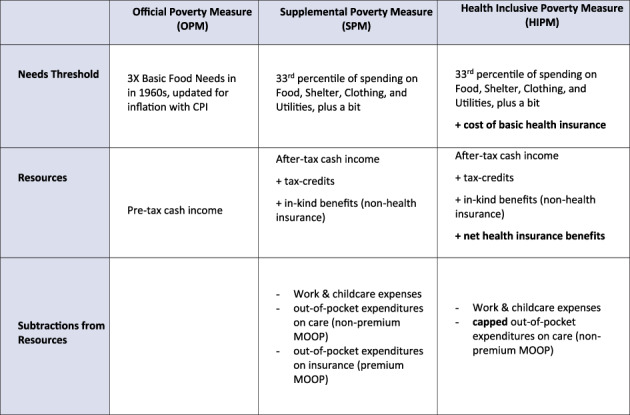
Overview of Poverty Measures: OPM, SPM, and HIPM. Note: This figure is adapted from table 1 in Korenman, Remler and Hyson (2019) [Color figure can be viewed at wileyonlinelibrary.com]

TABLE A1.

Propensity score estimation models for nonelderly adults

		Disabled adults			Parents			Nondisabled adults without dependents
		Coeff	Std.Err	p	Coeff	Std.Err	p	Coeff	Std.Err	p
	Medicare	−0.849	0.057	0.000	−0.760	0.271	0.005	−0.409	0.119	0.001
Health status	Excellent	−0.669	0.125	0.000	−0.084	0.047	0.073	−0.248	0.047	0.000
	Very good	−0.506	0.093	0.000
	Good	−0.183	0.064	0.005	0.322	0.045	0.000	0.299	0.044	0.000
	Fair				0.629	0.072	0.000	0.748	0.063	0.000
	Poor	0.091	0.062	0.146	0.411	0.165	0.013	0.996	0.113	0.000
Age × gender	19–25 female	0.517	0.165	0.002	0.708	0.086	0.000	0.739	0.070	0.000
	19–25 male	0.555	0.157	0.000	0.419	0.149	0.005	0.681	0.069	0.000
	26–31 female	0.279	0.146	0.056	0.438	0.061	0.000	0.595	0.080	0.000
	26–31 male	0.281	0.154	0.067	0.159	0.088	0.071	0.231	0.082	0.005
	32–41 female	0.508	0.099	0.000				0.654	0.080	0.000
	32–41 male	0.554	0.109	0.000	−0.173	0.064	0.007	0.239	0.080	0.003
	42–51 female	0.101	0.085	0.237	−0.177	0.058	0.003	0.305	0.076	0.000
	42–51 male	−0.039	0.092	0.671	−0.203	0.068	0.003	0.161	0.083	0.051
	52–65 female				−0.294	0.092	0.001
	52–65 male	−0.218	0.067	0.001	−0.278	0.092	0.002	0.016	0.065	0.809
Income, % FPL	<100% FPL	6E‐01	1E‐01	1E‐08	0.833	0.070	0.000	0.575	0.070	0.000
	100–124	5E‐01	9E‐02	2E‐07	0.644	0.078	0.000	0.570	0.090	0.000
	125–149	3E‐01	1E‐01	3E‐03	0.582	0.071	0.000	0.620	0.079	0.000
	150 +
Income	Interest	−0.492	0.057	0.000	−0.594	0.041	−14.511	−0.517	0.039	0.000
	Dividends	−0.125	0.107	0.242	−0.324	0.082	−3.929	−0.282	0.069	0.000
	Total	−0.490	0.109	0.000	0.000	0.000	−13.085
Education	Less than HS	0.780	0.082	0.000	0.610	0.062	9.792	0.143	0.036	0.000
	HS graduate	0.330	0.067	0.000	0.470	0.045	10.344	0.825	0.060	0.000
	Some college							0.468	0.045	0.000
Citizen		0.223	0.124	0.072	0.225	0.057	3.979
Household size		0.012	0.028	0.674	0.086	0.016	5.434	0.279	0.057	0.000
Race and ethnicity	Hispanic	0.442	0.327	0.176	−0.635	0.213	−2.979	0.055	0.163	0.736
	Black	0.458	0.330	0.164	−0.413	0.212	−1.951	0.064	0.163	0.696
	Asian	0.237	0.357	0.507	−0.727	0.226	−3.214	−0.117	0.175	0.502
	White	0.248	0.334	0.457	−0.718	0.218	−3.293	−0.318	0.169	0.060
Medicaid eligibility		0.042	0.098	0.665	0.508	0.059	8.541	0.234	0.070	0.001
Student		−0.280	0.258	3E‐01	0.208	0.133	1.564	−0.172	0.062	0.005
Full‐time work		−1.488	0.089	2E‐62	−0.396	0.042	−9.469	−0.927	0.040	0.000
Married		−0.540	6E‐02	4E‐17	−0.450	0.050	−8.948	−0.119	0.054	0.026
Pregnant					0.124	0.084	1.480	1.168	0.226	0.000
State fixed effects		+			+			+
Constant		−0.231	0.369	0.532	−0.617	0.242	−2.551	−2.012	0.196	0.000

Note: Table presents model of propensity score, estimating propensity to have Medicaid in the 2016 Current Population Survey's Annual Social and Economic Supplement. Regression run as a linear probability model (using ordinary least squares) on dependent binary indicator of Medicaid coverage. Std.Err is the standard error.

TABLE A2.

Propensity Score Estimation Models for Children and Elderly Adults

		Elderly Adults			Children
		Coeff	Std.Err	p	Coeff	Std.Err	p
	Medicare	0.279	0.088	0.002	−1.120	0.181	0.000
Health status	Excellent	−0.421	0.145	0.004
	Very good	−0.399	0.099	0.000	0.126	0.026	0.000
	Good				0.444	0.032	0.000
	Fair	0.506	0.076	0.000	0.799	0.091	0.000
	Poor	0.947	0.086	0.000	1.451	0.219	0.000
Age × gender	0–2 female				0.063	0.061	0.294
	0–2 male				0.084	0.059	0.157
	2–6 female				0.068	0.044	0.119
	2–6 male				0.067	0.044	0.123
	6–13 female				0.012	0.036	0.742
	6–13 male
	13–19 female				−0.112	0.041	0.007
	13–19 male				−0.172	0.041	0.000
	65–75 female
	65–75 male	0.070	0.078	0.373
	75+ female	−0.246	0.080	0.002
	75+ male	−0.275	0.093	0.003
Income, % FPL	<100% FPL				1.209	0.033	0.000
	100–124				0.741	0.045	0.000
	125+				0.550	0.044	0.000
Income	Interest	−0.802	0.069	0.000	−0.668	0.025	0.000
	Dividends	−0.350	0.127	0.006	−0.500	0.047	0.000
	Total	0.000	0.000	0.000	0.000	0.000	0.000
Education	Less than HS	0.768	0.091	0.000	0.757	0.472	0.108
	HS graduate	0.139	0.083	0.094	0.493	0.478	0.303
	Some college
Citizen		−0.490	0.109	0.000	0.567	0.070	0.000
Household size		0.079	0.070	0.261	−0.045	0.008	0.000
Race and ethnicity	Hispanic	0.200	0.355	0.574	−0.265	0.119	0.026
	Black	−0.053	0.356	0.882	−0.388	0.118	0.001
	Asian	0.377	0.374	0.313	−0.921	0.132	0.000
	White	−0.408	0.363	0.262	−0.769	0.123	0.000
Imputed medicaid eligibility		0.856	0.076	0.000	1.232	0.035	0.000
Student					−0.187	0.044	0.000
Married		−0.327	0.092	0.000
State‐fixed effects		+			+
Constant		−1.586	0.408	0.000	−1.946	0.494	0.000

Note: Table presents model of propensity score, estimating propensity to have Medicaid in the 2016 Current Population Survey's Annual Social and Economic Supplement. Regression run as a linear probability model (using ordinary least squares) on dependent binary indicator of Medicaid coverage. Std.Err is the standard error. Education of children represents highest level of parents' education.

TABLE A3.

Balance of matching variables, children's sample

		Decile 1 low likelihood Medicaid		Decile 5 medium likelihood Medicaid		Decile 10 high likelihood Medicaid
		No Medicaid	Medicaid	No Medicaid	Medicaid	No Medicaid	Medicaid
Age		9.69	9.81	8.76	8.67	7.24	7.17
Male		0.52	0.53	0.49	0.49	0.51	0.48
Race	Hispanic	0.10	0.18	0.36	0.35	0.58	0.61
	White	0.71	0.59	0.36	0.39	0.06	0.07
	Black	0.07	0.11	0.19	0.18	0.33	0.30
	Other race	0.12	0.12	0.09	0.09	0.03	0.02
Household income		155,987	140,610	39,986	37,701	15,455	16,133
Citizen		0.98	0.96	0.95	0.95	1.00	1.00
Imputed Medicaid eligibility		0.02	0.06	1.00	1.00	1.00	1.00
Health	Excellent	0.63	0.55	0.45	0.47	0.26	0.13
	Very good	0.28	0.31	0.33	0.31	0.21	0.20
	Good	0.08	0.12	0.20	0.19	0.43	0.52
	Fair or poor	0.00	0.01	0.02	0.02	0.10	0.14
Any dividend income		0.32	0.21	0.02	0.01	0.00	0.00
Any interest income		0.91	0.83	0.34	0.37	0.01	0.00
Official poverty status	Poor	0.00	0.00	0.28	0.32	0.99	0.97
	100%–125% FPL	0.00	0.00	0.18	0.19	0.01	0.02
	125%–150% FPL	0.00	0.00	0.23	0.18	0.00	0.00
	150% FPL +	1.00	1.00	0.31	0.30	0.00	0.00

Note: Table presents degree of balance in matched variables among children, across deciles of the estimated propensity to have Medicaid. Medicaid beneficiaries are matched to otherwise‐similar nonbeneficiaries within propensity deciles to simulate counterfactual poverty without the Medicaid program. Data from the authors' analysis of the 2016 Current Population Survey's Annual Social and Economic Supplement.

TABLE A4.

Balance of matching variables, adults with a disability sample

		Decile 1 low likelihood Medicaid		Decile 5 medium likelihood Medicaid		Decile 10 high likelihood Medicaid
		No Medicaid	Medicaid	No Medicaid	Medicaid	No Medicaid	Medicaid
Age		49.94	48.73	48.20	48.04	38.25	39.57
Male		0.48	0.52	0.53	0.45	0.29	0.41
Race	Hispanic	0.08	0.10	0.16	0.15	0.23	0.27
	White	0.75	0.70	0.53	0.56	0.36	0.35
	Black	0.11	0.12	0.25	0.20	0.30	0.31
	Other race	0.07	0.08	0.06	0.08	0.11	0.07
Household income		98,429	78,963	29,231	32,300	13,065	14,301
Citizen		0.96	0.94	0.94	0.96	0.91	0.96
Imputed Me dicaid eligibility		0.03	0.06	0.39	0.36	0.80	0.80
Health	Excellent	0.13	0.06	0.03	0.05	0.00	0.00
	Very good	0.22	0.16	0.07	0.05	0.00	0.03
	Good	0.28	0.29	0.21	0.20	0.23	0.21
	Fair or poor	0.37	0.48	0.69	0.70	0.77	0.76
Dividend income		0.22	0.17	0.03	0.04	0.00	0.00
Interest income		0.82	0.73	0.27	0.27	0.04	0.03
Official poverty status	Poor	0.03	0.05	0.48	0.44	0.84	0.86
	100%–125% FPL	0.02	0.02	0.11	0.12	0.09	0.09
	125%–150% FPL	0.03	0.05	0.11	0.09	0.05	0.03
	150% FPL +	0.93	0.88	0.31	0.34	0.03	0.02
Full‐time work		0.49	0.29	0.02	0.03	0.00	0.00
Married		0.66	0.60	0.29	0.29	0.06	0.06
Education	No HS degree	0.05	0.10	0.29	0.20	0.55	0.57
	HS degree	0.52	0.55	0.62	0.66	0.41	0.41
	Any college	0.44	0.35	0.10	0.14	0.04	0.02

Note: Table presents degree of balance in matched variables among adults with a disability, across deciles of the estimated propensity to have Medicaid. Medicaid beneficiaries are matched to otherwise‐similar non‐beneficiaries within propensity‐deciles to simulate counterfactual poverty without the Medicaid program. Data from the authors' analysis of the 2016 Current Population Survey's Annual Social and Economic Supplement.

TABLE A5.

Balance of matching variables, parents sample

		Decile 1 low likelihood Medicaid		Decile 5 medium likelihood Medicaid		Decile 10 high likelihood Medicaid
		No Medicaid	Medicaid	No Medicaid	Medicaid	No Medicaid	Medicaid
Age		41.93	39.78	36.74	36.37	29.42	30.37
Male		0.51	0.52	0.30	0.29	0.12	0.10
Race	Hispanic	0.12	0.21	0.35	0.38	0.45	0.40
	White	0.71	0.61	0.37	0.41	0.18	0.22
	Black	0.07	0.08	0.19	0.13	0.32	0.32
	Other race	0.10	0.10	0.09	0.08	0.04	0.07
Household income		148,558	129,731	40,564	39,980	14,424	15,446
Citizen		0.91	0.84	0.79	0.77	0.79	0.86
Imputed Medicaid eligibility		0.00	0.03	0.44	0.50	1.00	0.99
Health	Excellent	0.39	0.34	0.26	0.28	0.12	0.17
	Very good	0.40	0.34	0.29	0.31	0.33	0.17
	Good	0.19	0.30	0.35	0.31	0.37	0.45
	Fair or poor	0.03	0.03	0.11	0.10	0.19	0.20
Dividend income		0.30	0.23	0.02	0.02	0.01	0.00
Interest income		0.87	0.78	0.30	0.35	0.03	0.02
Official poverty status	Poor	0.00	0.02	0.31	0.29	0.91	0.87
	100%–125% FPL	0.00	0.00	0.14	0.17	0.04	0.08
	125%–150% FPL	0.01	0.01	0.19	0.17	0.05	0.04
	150% FPL +	0.99	0.97	0.37	0.37	0.00	0.01
Full‐time work		0.84	0.76	0.49	0.50	0.13	0.13
Married		0.93	0.91	0.62	0.62	0.24	0.23
Education	No HS degree	0.03	0.08	0.23	0.19	0.43	0.39
	HS degree	0.27	0.38	0.60	0.59	0.53	0.59
	Any college	0.70	0.55	0.17	0.22	0.04	0.02

Note: Table presents degree of balance in matched variables among parents, across deciles of the estimated propensity to have Medicaid. Medicaid beneficiaries are matched to otherwise‐similar nonbeneficiaries within propensity deciles to simulate counterfactual poverty without the Medicaid program. Data from the authors' analysis of the 2016 Current Population Survey's Annual Social and Economic Supplement.

TABLE A6.

Balance of matching variables, nondisabled adults without dependents sample

		Decile 1 low likelihood Medicaid		Decile 5 medium likelihood Medicaid		Decile 10 high likelihood Medicaid
		No Medicaid	Medicaid	No Medicaid	Medicaid	No Medicaid	Medicaid
Age		44.18	41.77	35.56	36.16	31.17	31.99
Male		0.55	0.57	0.51	0.50	0.41	0.37
Race	Hispanic	0.09	0.11	0.28	0.30	0.44	0.51
	White	0.75	0.72	0.47	0.39	0.21	0.19
	Black	0.09	0.08	0.17	0.16	0.26	0.22
	Other Race	0.07	0.08	0.08	0.15	0.09	0.07
Household income		129,088	127,313	54,706	51,938	19,136	18,450
Citizen		0.94	0.91	0.87	0.85	0.86	0.88
Imputed Medicaid eligibility		0.00	0.02	0.18	0.20	0.93	0.96
Health	Excellent	0.38	0.35	0.25	0.29	0.13	0.08
	Very good	0.39	0.32	0.30	0.26	0.19	0.24
	Good	0.20	0.29	0.33	0.27	0.40	0.41
	Fair or poor	0.03	0.04	0.12	0.18	0.28	0.27
Dividend income		0.27	0.24	0.04	0.04	0.00	0.00
Interest income		0.84	0.85	0.41	0.40	0.05	0.06
Official poverty status	Poor	0.01	0.04	0.25	0.23	0.75	0.76
	100%–125% FPL	0.00	0.00	0.07	0.07	0.09	0.13
	125%–150% FPL	0.00	0.01	0.07	0.07	0.12	0.09
	150% FPL +	0.98	0.95	0.61	0.63	0.03	0.02
Full‐time Work		0.88	0.81	0.27	0.31	0.01	0.01
Married		0.52	0.51	0.27	0.24	0.16	0.18
Education	No HS degree	0.03	0.06	0.17	0.16	0.45	0.42
	HS degree	0.39	0.43	0.66	0.68	0.52	0.53
	Any college	0.58	0.51	0.16	0.16	0.03	0.05

Note: Table presents degree of balance in matched variables among nondisabled, nonelderly, nonparents adult sample, across deciles of the estimated propensity to have Medicaid. Medicaid beneficiaries are matched to otherwise‐similar nonbeneficiaries within propensity‐deciles to simulate counterfactual poverty without the Medicaid program. Data from the authors' analysis of the 2016 Current Population Survey's Annual Social and Economic Supplement.

TABLE A7.

Balance of matching variables, adults 65 years and older sample

		Decile 1 low likelihood Medicaid		Decile 5 medium likelihood Medicaid		Decile 10 high likelihood Medicaid
		No Medicaid	Medicaid	No Medicaid	Medicaid	No Medicaid	Medicaid
Age		73.21	72.90	73.85	73.95	72.72	72.61
Male		0.47	0.50	0.41	0.39	0.37	0.33
Race	Hispanic	0.02	0.05	0.20	0.16	0.59	0.47
	White	0.91	0.83	0.53	0.52	0.10	0.12
	Black	0.04	0.05	0.18	0.22	0.16	0.09
	Other race	0.03	0.07	0.09	0.09	0.15	0.33
Household income		92,476	93,580	35,814	32,123	19,328	20,573
Citizen		0.99	0.99	0.93	0.91	0.63	0.67
Imputed medicaid eligibility		0.01	0.02	0.18	0.17	0.79	0.75
Health	Excellent	0.18	0.12	0.04	0.05	0.02	0.00
	Very Good	0.37	0.33	0.09	0.09	0.01	0.00
	Good	0.35	0.38	0.34	0.25	0.17	0.13
	Fair or poor	0.10	0.17	0.53	0.61	0.79	0.87
Dividend income		0.40	0.41	0.02	0.03	0.00	0.00
Interest income		0.92	0.82	0.25	0.26	0.00	0.04
Official poverty status	Poor	0.01	0.06	0.21	0.31	0.74	0.71
	100%–125% FPL	0.02	0.04	0.10	0.15	0.07	0.06
	125%–150% FPL	0.03	0.03	0.10	0.13	0.05	0.06
	150% FPL +	0.94	0.86	0.58	0.40	0.14	0.16
Full‐time Work		0.19	0.21	0.05	0.06	0.03	0.01
Married		0.70	0.70	0.43	0.39	0.30	0.40
Education	No HS degree	0.03	0.05	0.36	0.36	0.87	0.87
	HS degree	0.48	0.46	0.48	0.55	0.09	0.08
	Any college	0.49	0.49	0.16	0.09	0.04	0.04

Note: Table presents degree of balance in matched variables among adults age 65 plus, across deciles of the estimated propensity to have Medicaid. Medicaid beneficiaries are matched to otherwise‐similar nonbeneficiaries within propensity‐deciles to simulate counterfactual poverty without the Medicaid program. Data from the authors' analysis of the 2016 Current Population Survey's Annual Social and Economic Supplement.

Zewde N, Remler D, Hyson R, Korenman S. Improving estimates of Medicaid's effect on poverty: Measures and counterfactuals. Health Serv Res. 2021;56(6):1190‐1206. 10.1111/1475-6773.13699

REFERENCES

- 1. Allen H, Swanson A, Wang J, Gross T. Early Medicaid expansion associated with reduced payday borrowing in California. Health Aff. 2017;36(10):1769‐1776. 10.1377/hlthaff.2017.0369 [DOI] [PubMed] [Google Scholar]
- 2. Antonisse L, Garfield R, 2018. The Effects of Medicaid Expansion under the ACA: Updated Findings from a Literature Review Kaiser Family Foundation. 2018. https://www.kff.org/medicaid/issue-brief/the-effects-of-medicaid-expansion-under-the-aca-updated-findings-from-a-literature-review-march-2018/. Accessed April 1, 2019.
- 3. Miller S, Wherry LR. Health and access to care during the first 2 years of the ACA Medicaid expansions. N Engl J Med. 2017;376(10):947‐956. 10.1056/NEJMsa1612890 [DOI] [PubMed] [Google Scholar]
- 4. Sommers BD, Baicker K, Epstein AM. Mortality and access to care among adults after state Medicaid expansions. N Engl J Med. 2012;367(11):1025‐1034. 10.1056/NEJMsa1202099 [DOI] [PubMed] [Google Scholar]
- 5. Winkelman TNA, Segel JE, Davis MM. Medicaid enrollment among previously uninsured Americans and associated outcomes by race/ethnicity—United States, 2008‐2014. Health Serv Res. 2019;54(Suppl 1):297‐306. 10.1111/1475-6773.13085 [DOI] [PMC free article] [PubMed] [Google Scholar]
- 6. Zewde N, Eliason E, Allen H, Gross T. The effects of the ACA Medicaid expansion on Nationwide home evictions and eviction‐court initiations: United States, 2000‐2016. Am J Public Health. 2019;109(10):1379‐1383. 10.2105/AJPH.2019.305230 [DOI] [PMC free article] [PubMed] [Google Scholar]
- 7. Sommers BD, Oellerich D. The poverty‐reducing effect of Medicaid. J Health Econ. 2013;32(5):816‐832. 10.1016/j.jhealeco.2013.06.005 [DOI] [PubMed] [Google Scholar]
- 8. Zewde N, Wimer C. Antipoverty impact of Medicaid growing with state expansions over time. Health Aff. 2019;38(1):132‐138. 10.1377/hlthaff.2018.05155 [DOI] [PubMed] [Google Scholar]
- 9. Short K. The Research Supplemental Poverty Measure: 2011. US Census Bureau. 2012. https://www.census.gov/library/publications/2012/demo/p60-244.html. Accessed February 24, 2021.
- 10. National Academies of Sciences, Engineering, and Medicine . A Roadmap to Reducing Child Poverty. Washington, DC: The National Academies Press; 2019. 10.17226/25246. [DOI] [PubMed] [Google Scholar]
- 11. Korenman SD, Remler DK. Including health insurance in poverty measurement: the impact of Massachusetts health reform on poverty. J Health Econ. 2016;50:27‐35. 10.1016/j.jhealeco.2016.09.002 [DOI] [PubMed] [Google Scholar]
- 12. Interagency Technical Working Group on Evaluating Alternative Measures of Poverty . Final Report of the Interagency Technical Working Group on Evaluating Alternative Measures of Poverty. Office of the Chief Statistician of the United States. 2021. https://www.bls.gov/cex/itwg-report.pdf
- 13. Remler DK, Korenman SD, Hyson RT. Estimating the effects of health insurance and other social programs on poverty under the affordable care act. Health Aff. 2017;36(10):1828‐1837. 10.1377/hlthaff.2017.0331 [DOI] [PubMed] [Google Scholar]
- 14. Korenman S, Remler DK, Hyson RT. Accounting for the impact of Medicaid on child poverty. National Bureau of Economic Research. 2019. 10.3386/w25973 [DOI]
- 15. Korenman S, Remler DK, Hyson RT. Medicaid expansions and poverty: comparing supplemental and health‐inclusive poverty measures. Soc Serv Rev. 2019;93(3):429‐483. 10.1086/705319 [DOI] [Google Scholar]
- 16. Fox L. The Supplemental Poverty Measure: 2019. 2020. https://www.census.gov/library/publications/2020/demo/p60‐272.html. Accessed February 27, 2021.
- 17. Korenman S, Remler DK, Hyson RT. The Impact of Health Insurance and Other Social Benefits on Poverty in New York State. 2018. www2.cuny.edu/wp‐content/uploads/sites/4/page‐assets/about/centers‐and‐institutes/demographic‐research/New‐York‐HIPM_2018‐08‐06.pdf
- 18. Decker SL, Lipton BJ, Sommers BD. Medicaid expansion coverage effects grew in 2015 with continued improvements in coverage quality. Health Aff. 2017;36(5):819‐825. 10.1377/hlthaff.2016.1462 [DOI] [PubMed] [Google Scholar]
- 19. Sullivan L, Meschede T, Shapiro T, Kroeger T, Escobar F. Not Only Unequal Paychecks: Occupational Segregation, Benefits, and the Racial Wealth Gap. Institute on Assets and Social Policy. 2019. https://heller.brandeis.edu/iasp/pdfs/racial‐wealth‐equity/asset‐integration/occupational_segregation_report_40219.pdf. Accessed January 23, 2019.
- 20. Robert Wood Johnson Foundation. HIX Compare 2015. Dataset. Published April 26, 2017. http://www.rwjf.org/en/library/research/2017/04/hix-compare-2014-2017-datasets.html. Accessed April 4, 2019.
- 21. National Bureau of Economic Research. CMS Landscape Files Data ‐ Descriptions of the Drug Plans . Published 2016. http://www.nber.org/data/cms‐landscape‐files‐data.html. Accessed April 4, 2019.
- 22. Brooks T, Touschner J, Artiga S, Stephens J, Gates A. Modern Era Medicaid: Findings from a 50‐State Survey of Eligibility, Enrollment, Renewal, and Cost‐Sharing Policies in Medicaid and CHIP as of January 2015. The Henry J. Kaiser Family Foundation Published January 20, 2015. https://www.kff.org/health‐reform/report/modern‐era‐medicaid‐findings‐from‐a‐50‐state‐survey‐of‐eligibility‐enrollment‐renewal‐and‐cost‐sharing‐policies‐in‐medicaid‐and‐chip‐as‐of‐january‐2015/. Accessed April 4, 2019.
- 23. Flood S, King M, Rodgers R, Ruggles S, Warren JR. Integrated Public Use Microdata Series, Current Population Survey: Version 6.0. Published online 2018. 10.18128/D030.V6.0 [DOI]
- 24. Borjas GJ. The labor supply of undocumented immigrants. Labour Econ. 2017;46:1‐13. 10.1016/j.labeco.2017.02.004 [DOI] [Google Scholar]
- 25. Semega J, Kollar M, Creamer J, Mohanty A. Income and Poverty in the United States: 2018. US Census Bureau. 2019. https://www.census.gov/library/publications/2019/demo/p60-266.html. Accessed September 25, 2019.
- 26. National Research Council . In: Citro CF, Michael RT, eds. Measuring Poverty: A New Approach. Washington, DC: The National Academies Press; 1995. https://www.nap.edu/catalog/4759/measuring-poverty-a-new-approach [Google Scholar]
- 27.Yan T. In: Lavrakas P, ed. Hot‐deck imputation. In: Encyclopedia of Survey Research Methods. Vol 1. SAGE Publications, Inc; 2008;316‐317. 10.4135/9781412963947.n212 [DOI] [Google Scholar]
- 28. Baicker K, Finkelstein A, Song J, Taubman S. The impact of Medicaid on labor market activity and program participation: evidence from the Oregon health insurance experiment. Am Econ Rev. 2014;104(5):322‐328. [DOI] [PMC free article] [PubMed] [Google Scholar]
- 29. Ben‐Shalom Y, Moffitt R, Scholz JK. An assessment of the effectiveness of antipoverty programs in the United States. The Oxford Handbook of the Economics of Poverty Published Online November 5, 2012. 10.1093/oxfordhb/9780195393781.013.0023 [DOI]
- 30. Remler D, Korenman S, Hyson RT. How Does the Implicit Insurance of Free Care Affect Poverty? Methods for Incorporating Free Care into the Health‐Inclusive Poverty. 2020.