Switched forced SEIRDV compartmental models to monitor COVID-19 spread and immunization in Italy

Abstract

This paper presents a new hybrid compartmental model for studying the COVID-19 epidemic evolution in Italy since the beginning of the vaccination campaign started on 2020/12/27 and shows forecasts of the epidemic evolution in Italy in the first six months. The proposed compartmental model subdivides the population into six compartments and extends the SEIRD model proposed in [E.L.Piccolomini and F.Zama, PLOS ONE, 15(8):1–17, 08 2020] by adding the vaccinated population and framing the global model as a hybrid-switched dynamical system. Aiming to represent the quantities that characterize the epidemic behaviour from an accurate fit to the observed data, we partition the observation time interval into sub-intervals. The model parameters change according to a switching rule depending on the data behaviour and the infection rate continuity condition. In particular, we study the representation of the infection rate both as linear and exponential piecewise continuous functions. We choose the length of sub-intervals balancing the data fit with the model complexity through the Bayesian Information Criterion. We tested the model on italian data and on local data from Emilia-Romagna region. The calibration of the model shows an excellent representation of the epidemic behaviour in both cases. Thirty days forecasts have proven to well reproduce the infection spread, better for regional than for national data. Both models produce accurate predictions of infected, but the exponential-based one perform better in most of the cases. Finally, we discuss different possible forecast scenarios obtained by simulating an increased vaccination rate.

1. Introduction

Compartmental models are essential mathematical tools in the analysis of the evolution of epidemics, for prediction and simulation of future strategies which can be used by governments and policymakers to allocate sanitary and economic resources. The parameters of such models are related to meaningful characteristics of the epidemic disease, such as infection rate, infectious period, lethality rate. Moreover, through such models, it is possible to estimate the number of secondary cases produced by a single infected person at start time (basic reproduction number R₀) and during the epidemic evolution (effective time-dependent reproduction number R_t). In particular, the trend of R_t is of great importance to check the epidemic evolution over time.

The COVID-19 pandemic, caused by the Sars-CoV-2 virus, has renewed interest in studying these models and a significant number of papers appeared on this subject since the beginning of 2020 (refer to LitCovid database for up to date literature (Chen, Allot & Lu, 2020)). They differ each other for the type of model proposed, the external events considered, such as movement restrictions imposed by governments or quarantines, and the regions where models are applied.

Starting from the first SIR (susceptible (S), infected (I), and recovered (R)) model, proposed in 1927 by Kermack and McKendrick (Kermack & McKendrick, 1927), several generalizations have been formulated over the years by increasing the number of compartments, such as, for example, the susceptible – exposed – infectious – recovered (SEIR) and the susceptible - exposed - infected - recovered - dead (SEIRD) schemes. Further extensions have been proposed to model the COVID-19 outbreak considering the different social distancing policies and control measures applied in the various geographic areas to contain the epidemic spread. More compartments have been added, making the models more and more complex (see (Parolini et al., 2021; Zhu & Gallego, 2021; Friji, Hamadi, Ghazzai, Besbes, & Massoud, 2021; Giordano et al., 2021), to mention only a few of the most recent).

In this paper we intend to consider the effects of the vaccine on the epidemic spread during the first months since the vaccination campaign started. We introduce a new scheme, named SEIRDV, that extends the SEIRD model with the compartment of vaccinated people. Among the vaccine-related papers within the COVID-19 literature several hypothetical scenarios are analysed based on different prioritisation policies according to vaccine efficacy and its availability (Roy, Dutta, & Ghosh, 2021). Other papers focus on the possible benefits of combining vaccination with nonpharmaceutical interventions (NPIs) such as surveillance, social distancing, social relaxation, quarantining, patient treatment/isolation (see (Acuña-Zegarra, Díaz-Infante, Baca-Carrasco, & Liceaga, 2021; Rachaniotis, Dasaklis, Fotopoulos, & Tinios, 2021) and references therein). Following the approach in (Goebel, Sanfelice, & Teel., 2012), we introduce a switching rule that governs the SEIRDV model state at any given time. Besides producing optimal fit to epidemic data, introducing such a hybrid approach allows us to represent disease evolution when restriction policies and virus variants cause changes in fundamental parameters such as infection rate, recovery periods, and death rates. Although switched models are widespread in various engineering applications, studies about epidemic models are less common; see, for example (Liu & Stechlinski, 2012), (SIRV) (El Koufi, Bennar & N. Yousfi, 2021)(SIR) and (Maher et al., 2021) (SEIRD). In particular the authors in (Maher, Majdalawieh, & Nizamuddin, 2021) propose a hybrid SEIRD model with a mortality rate represented by an inverse exponential function where the residual correction is based on the ARIMA method. The model, tested on US COVID-19 statistic data in the period February–September 2020, made precise predictions for up to 2 months ahead. The reader can also refer to (Maher et al., 2021) for an exhaustive bibliography.

Concerning the model parameters, it is well known that COVID-19 epidemic data cannot be accurately represented by any compartmental approach with constant parameters all over the epidemic duration. To face this problem, some authors use variable parameters in the time interval (for example (Giordano et al., 2021)) or change the fitting function (see (Friji et al., 2021)). In our approach all the model parameters are constant in each switching time interval, except for the infection rate which is a time-dependent forcing function modelled as piecewise continuous.

The model calibration is carried out by solving a sequence of constrained minimizations of the weighted least-squares residuals between the measured epidemic data and the value of the state variables, which satisfy the initial value ordinary differential system representing the SEIRDV model.

This paper is an extension of our previous work (Piccolomini and Zama, 2020), where we proposed a SEIRD model (before the availability of vaccines), with two different forcing functions, to monitor the first phase of the evolution of COVID-19 in Italy (2020/02/24–2020/05/24). Compared to (Piccolomini and Zama, 2020) we modify the model as follows: we include the vaccinated compartment, we represent the proposed scheme into the hybrid models theoretical frame, and finally we change the expression of the forcing functions. Moreover in the calibration phase, we add weights in the fitting objective function and bounded constraints, thus improving the model computational effectiveness and accuracy.

In the experimental section, we report the results obtained by our simulations on the Italian national and regional epidemic data in the period 2020/12/27–2021/06/17. The inclusion of two different expressions for the infection rate function allows us to obtain different possible scenarios which prove to be very useful in the prediction phase. Concerning the effectiveness of COVID-19 vaccines, recent studies (Lopez Bernal et al., 2021) have shown its relation to the new Sars-Cov-2 variants and the type of Vaccines used. Following (Cai, Li, & Song, 2018) we test an extension of SEIRDV, which includes vaccination efficiency and report prediction results using the values reported in (Lopez Bernal et al., 2021). No significant change is observed in the prediction phase since the vaccination campaign is at its first beginning. Nevertheless, we believe that such an extension and the distinction in vaccination doses and ages will significantly improve the monitoring of the autumn-winter epidemic spread.

1.1. Contributions

We summarize here the main contributions of this paper.

• ●We propose a SEIRDV scheme by adding the Vaccinated compartment to the well known SEIRD model.
• ●We consider a dynamical switched framework where the interval length is chosen on the basis of the Bayesian Information Criterium.
• ●We represent the infection rate as a continuous time dependent function comparing a linear and an exponential piecewise formulation.
• ●We introduce a model extension that takes into account the reduced vaccine efficacy and present a preliminary experiment in the hypothesis of mass vaccination with a single vaccine dose.

1.2. Limitations

The present study is concerned with modelling and prediction COVID-19 evolution during the first six month of vaccination campaign in Italy. We consider vaccination data regarding a single vaccine dose without distinguishing the vaccine type.

The rest of the paper is organized as follows. In Section 2, we present the proposed switched SEIRDV model; in Section 3 we describe the calibration procedure implemented and the results obtained on data from Italy and Emilia-Romagna region. The results of prevision on the same data are reported in Section 4 and conclusions are drawn in Section 5. Finally Appendix A concerns the SEIRDV model with constant parameters and Appendix B reports an extension of the SEIRDV model considering a partial vaccine efficacy.

2. Switched forced SEIRDV model

The movement restriction policies adopted worldwide as well as the occurrence of different virus variants cause changes in the value of the infection rate and possibly of other model parameters over time. In order to monitor the model parameters from the measured data flexibly, we propose a hybrid switched SEIRDV compartmental model and represent the infection rate as a continuous time-dependent function, modelled according to the epidemic data. Given the SEIRDV compartmental model (A.1) described in appendix Appendix A, with parameters (α, β, γ, η, ν), we split the time interval [t₀, T] into p sub-intervals Δ_k = [t_k−1, t_k] (k = 1, …, p and t_p = T) and define a switching rule Θ setting the values of the model parameters as follows:

$$\mathrm{\Theta }(t)={({\alpha }_k,{\beta }_k,{\gamma }_k,{\eta }_k,{\nu }_k)}^T,t\in {\mathrm{\Delta }}_k.$$

Then the hybrid model is represented as (Goebel et al., 2012):

$$\left(\begin{array}{c}{u}^{\prime }\\ {\mathrm{\Theta }}^{\prime }\end{array}\right)=\left(\begin{array}{c}{F}_{\mathrm{\Theta }}(t,u)\\ \mathbf{0}\end{array}\right),u=(S(t),E(t),I(t),R(t),D(t),V(t))$$ (1)

with state variable (u,Θ)^T and F_Θ(t, u) is the right-hand-side of system (A.1), and with model parameters represented by the piecewise constant function Θ(t).

However, using a constant value for the infection rate β_k does not represent the epidemic behaviour in a sufficiently flexible way (Piccolomini and Zama, 2020); therefore, we introduce a continuous time-dependent infection rate β(t). In this case, the epidemic model is known in the literature as forced model (see for example (Keeling & Rohani, 2011) chp 6). In this paper, we represent the infection rate as piecewise linear and exponential interpolating functions, yielding to SEIRDV_pwl and SEIRDV_pwe models, respectively.

Let us define β_k(t) the restriction of β(t) to the interval Δ_k, k = 1, …, p, and set the values β_k ≡β(t_k), k = 0, …, p . The SEIRDV_pwl defines the infection rate as:

$${\mathit{\beta }}_k(t)=\frac{t-t_k}{t_{k-1}-t_k}{\beta }_{k-1}+\frac{t-t_{k-1}}{t_k-t_{k-1}}{\beta }_k,t\in {\mathrm{\Delta }}_k,$$ (2)

whereas SEIRDV_pwe defines the infection rate as follows:

$${\mathit{\beta }}_k(t)={\beta }_{k-1}{e}^{-\rho (t-t_{k-1})/(t_k-t_{k-1})},\rho =-\log \left(\frac{{\beta }_k}{{\beta }_{k-1}}\right),t\in {\mathrm{\Delta }}_k.$$ (3)

We observe that for both models it holds:

$${\mathit{\beta }}_k(t_k)={\mathit{\beta }}_{k+1}(t_k),k=1,\dots ,p-1$$

hence β is continuous in [t₀, T].

The evolution of the global hybrid forced model, represented in Fig. 1, shows the changes of the epidemic model at each switching interval Δ_k represented by the values of the model parameters defined as Θ_k ≡Θ(t), t ∈ Δ_k.

Fig. 1.

The evolution of the global hybrid model, related to the values of the parameters Θ_k.

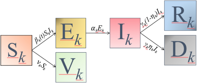
The restriction of the dynamical model (1) on each interval Δ_k, is represented in Fig. 2, where the model populations, for t ∈ Δ_k, are given by (S_k, E_k, I_k, R_k, D_k, V_k).

Fig. 2.

Dynamical model (1) restricted to the interval Δ_k.

3. Calibration of switched forced SEIRDV

This section focuses on the parameters calibration describing both the computational procedure in paragraph 3.1, and the numerical results in paragraph 3.2.

3.1. Calibration procedure

We describe the calibration procedure in the interval [t₀, T] supposed of n days. We calibrate the parameters on the sub-intervals Δ_k, k = 1, …p with uniform size L = ⌊n/p⌋ and n = L ⋅ p. In the case n ≠ L ⋅ p, the length of the last interval Δ_p is set as n − (p − 1)L if 0 < n − p ⋅ L ≤ ⌊L/2⌋. In the case n − L ⋅ p > ⌊L/2⌋, the number of the intervals is increased by one (p = p + 1), and the length of the last interval is n − (p − 1)L. In this way we avoid that the last interval is has too small with respect to the previous ones.

Generally, we are interested in keeping L as large as possible to guarantee a proper balancing between the data fit and the model complexity, evaluated in terms of the number of parameters to be calibrated. In paragraph 3.2 we discuss the details of the choice of a proper value for L.

Assuming mass vaccination and using the vaccination data V available from the databases, we can avoid the estimation of the parameter ν by rewriting the last equation of (A.1) as $V^{\prime }=\mathcal{U}$ and first equation of system (A.1) as follows:

$$S^{\prime }=-\frac{\beta }{N}SI-\mathcal{U}$$ (4)

where the function $\mathcal{U}(t)$ is the linear interpolation of the finite difference approximation of V′ at each day. Let V₁, V₂, …, V_n be the values obtained from the vaccination database on days 1, …, n, we consider the finite difference approximation of V′:

$$V_k^{\prime }=\left\{\begin{array}{cc}{V}_k-V_{k-1},& k=2,\dots ,n\\ 0,& k=1\end{array}\right)$$

We describe now the parameter estimation process in a single sub-interval Δ_k. We collect the observed data about infected, recovered, dead compartments in vectors I, R and D of size L and we stack them into the matrix $Y\in {\mathbb{R}}^{L\times 4}$, Y = [I, R, D, V]. Considering $Z\in {\mathbb{R}}^{L\times 4}$ as the restriction of u(t; Θ) (defined in (1) with F_Θ(t, u) given by (4)) to the components I(t), R(t), D(t), V(t) computed in Δ_k, we calculate the model parameters Θ_k = (α_k, β_k, γ_k, δ_k) solving a weighted constrained nonlinear least squares problem of the form:

$${\mathrm{\Theta }}_k=\arg \underset{\mathrm{\Theta }\in B}{\min }\sum _{j=1}^4\sum _{i=1}^L{(Z_{i,j}-Y_{i,j})}^2/{\mu }_j,{\mu }_j=\frac{1}{L}\sum _{i=1}^L{Y}_{i,j}.$$ (5)

where the positive weights μ_j are introduced to compensate different data scales. The bounded set B is defined as

$$B=\left\{\mathrm{\Theta }\in R^4:l{b}_i\le {\theta }_i\le u{b}_i,i=1,\dots ,4\right\}$$

where the upper bounds ub_i = 1, i = 1 …, 4 and lower bounds lb = [10⁻⁴, 10⁻⁴, 10⁻⁴, 0] guarantee that the values reported in the literature are contained, without imposing a too strict constraint.

To solve the minimization problem (5) numerically, we use iterative solvers as discussed in paragraph 3.2. Fig. 3 schematically represents the calibration steps of the global hybrid model in the whole interval [t₀, T]. The scheme highlights that the results Θ_k of the minimization problem on Δ_k is taken in input as starting guess in the minimization problem on Δ_k+1.

Fig. 3.

Calibration steps of the global hybrid model parameters Θ_k.

To suitably choose the first starting guess Θ₀, which has a fundamental role in the quality of the final solution, we compute the solution $\tilde{\mathrm{\Theta }}$ of problem (5) on a unique short time interval of about ten days using as starting guess (1/6, 0.02, 0.05, 0.001) as discussed in appendix Appendix A. We set ${\mathrm{\Theta }}_0=\tilde{\mathrm{\Theta }}$. The forward differential problem (4) is solved by a fourth order variable step Runge-Kutta method. The initial conditions in each sub-interval Δ_k are given by the observed values of the compartments I, R, D, V in the initial day of Δ_k.

Concerning the starting value E₀ of the exposed compartment which is not available from data, we propose a heuristic procedure by relating it with the delay time t_d between the contact with the infectious agent and the onset of symptoms of infection (see paragraph 3.2 for more details).

The starting value of susceptible S₀ is the difference between the total population N and the sum of all the other compartments at time t₀.

3.2. Results of calibration

The results presented in this section have been obtained by implementing the SEIRDV_pwl and SEIRDV_pwe algorithms in Matlab 2021a. The codes are available on https://github.com/fzama63/COVID-SEIRDV.

We highlight that a single vaccine dose is considered without distinction among the vaccine types. Since up to now there are not precise results about the vaccine immunity duration and efficacy, we suppose that the vaccine produces a complete unlimited immunization. In AppendixB we present a possible extension of the proposed model including limited vaccine efficacy and immunity duration. However, at the moment of these experiment the situation is not clearly defined and this extension will require a more detailed analysis.

3.2.1. Data description

Epidemic data are downloaded from the repository open source Github https://github.com/pcm-dpc/COVID-19 of the Italian Civil Protection Department, containing the official data provided by the Ministry of Health (see (Morettini, Sbrollin, Marcantoni & Burattini, 2020) for a detailed description). We consider here the global national data (N = 60360000) as well as the regional data from Emilia-Romagna (N = 4445900). Information about vaccine administration is obtained in the Github repository: https://github.com/italia/covid19-opendata-vaccini. Although most vaccines are administered in two different doses we consider, in our study, as vaccinated the people who received the first dose. We highlight that the vaccination campaign started quite slowly in Italy and that in the period of interest about 70% of vaccinated people had received only the first dose. Furthermore, little evidence of low vaccine efficacy or re-infection had been reported at that time and optimal immunization properties were reported after a single vaccine dose (see https://assets.publishing.service.gov.uk/government/uploads/system/uploads/attachment_data/file/986361/Vaccine_surveillance__report__week_19.pdf).

3.3. Metrics for results evaluation

To analyse the numerical solution of the calibration in the interval [t₀, T] constituted of n days, we compute, for any considered population, a relative residual defined as:

$$RRES=\frac{{\sum }_{i=1}^n{(X_i-X{d}_i)}^2}{{\sum }_{i=1}^{n}X{d}_i^2}$$

and the Bayesian Information Criterion (BIC) (Burnham & Anderson, 2004), defined as follows:

$$BIC(X)=N_{\theta }\log (n)+\log \left(\frac{{\sum }_{i=1}^n{(X_i-X{d}_i)}^2}{n}\right)$$

where N_θ is the number of the estimated parameters, Xd_i represents the acquired compartment data and X_i is the corresponding value computed by the calibrated model at day i, i = 1, …, n. The BIC takes into account the number of model estimated parameters and tends to penalize the inclusion of additional parameters. The lower this quantity, the better the model will be.

3.4. Implementation details

We have solved the constrained least squares problems (5) by means of the lsqnonlin Matlab function from the Optimization Toolbox compareing the trust-region reflective (TR) method with the Levemberg Marquardt (LM) one, which overperforms the Broyden-Fletcher-Goldfarb-Shanno (BFGS) as noted in (Friji et al., 2021).

The initial value differential problem (A.1) has been solved with the ode45 Matlab function.

To set a convenient initial value E₀ for the exposed compartment, in the hypothesis that previously acquired data is not available, and using the new infected value (I_new), available in the epidemic data repository, which represents the number of daily new cases. We test, for t_d = 1, …, 10, the SEIRDV_pwl and SEIRDV_pwe algorithms setting E₀ = I_new(t₀ + t_d) in a time interval of 30 days, from 2020/12/27 to 2021/01/26. Among the computed E₀ values, we choose the one minimising the RRES of the I compartment.

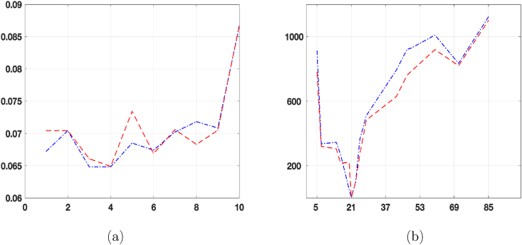
As shown in Fig. 4(a), the smallest RRES is obtained when t_d = 3 for SEIRDV_pwl with RRES = 0.064819 and when t_d = 4 for SEIRDV_pwe, with RRES = 0.064879. Hence we continue throughout this section setting E0 = 11223 with t_d = 3 and I given by SEIRDV_pwl.

Fig. 4.

(a): RRES vs t_d. (b): ∑Δ_BIC(X) vs L with X = (I, R, D). In both figures SEIRDV_pwl is plotted with blue dash-dotted line and SEIRDV_pwe with red dashed line.

3.5. Analysis of the results

We define the calibration period of n = 85 days, from 2020/12/27 to 2021/3/21 (we remind that in Italy vaccination campaign started on 2020/12/27) and run the calibration of SEIRDV_pwe and SEIRDV_pwl models.

The first aspect of our analysis concerns the choice of the number of switches. We split the whole time interval into sub-intervals of fixed length L (except for the last one which can be of different size). We observe that the number of parameters to be identified is proportional to the number of switches. Hence, increasing the number of switches, the computational cost raises whereas the fit error decreases. In order to choose the best value L we try all the values in the interval [5, 85] days and and choose L as:

$$L=\mathrm{arg\; min}\sum _{X=(I,R,D)}{\mathrm{\Delta }}_{BIC}(X)$$

where Δ_BIC(X) ≡ BIC(X) − BIC_min(X) and BIC_min(X) is the minimum BIC_min(X) all over the values of the interval days [5, 85].

Fig. 4(b) plots ∑_X=(I,R,D)Δ_BIC(X) in the interval [5, 85] with red dot-dashed line for SEIRDV_pwe and blue line for SEIRDV_pwl model. The minimum value is reached when L = 21, hence throughout this section, we split the calibration time into four sub-intervals of length L = 21 as follows:

$$\begin{array}{ccc}& {\mathrm{\Delta }}_1=[2020/12/27,2021/01/17]& {\mathrm{\Delta }}_2=[2021/01/17,2021/02/07]\\ & {\mathrm{\Delta }}_3=[2021/02/07,2021/02/28]& {\mathrm{\Delta }}_4=[2021/02/28,2021/03/21].\end{array}$$ (6)

We compare in Table 1 the two tested Levenberg- Marquardt and Trust-Region optimization algorithms, reporting the number of function evaluations FCount and the relative residual RRES for the infected, recovered and dead compartments. We find that for both exponential and linear infection rates, the TR method is computationally the most efficient (smallest number of function evaluations) and it is also slightly more precise than LM. Therefore we continue our analysis applying the TR method.

Table 1.

Number of function evaluations FCount and relative residual RRES obtained by LM and TR solvers for SEIRDV_pwl and SEIRDV_pwe. In bold the best results obtained for each algorithm.

model	method	FCount	RRES
			I	R	D
SEIRDV_pwl	TR	130	0.0083	0.0018	0.0009
	LM	4113	3926	0.0087	0.0021
SEIRDV_pwe	TR	125	0.0080	0.0018	0.0012
	LM	3928	0.0085	0.0020	0.0014

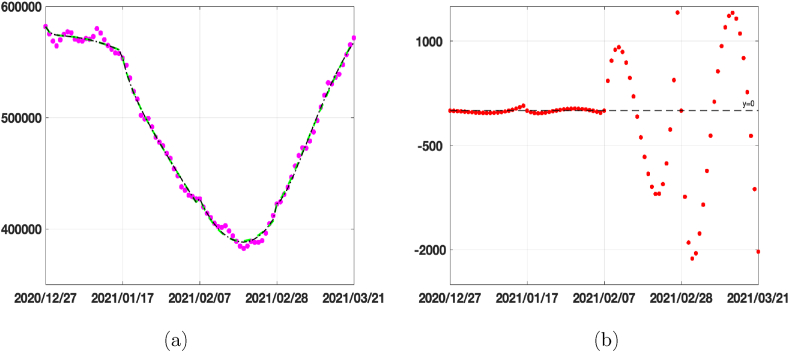
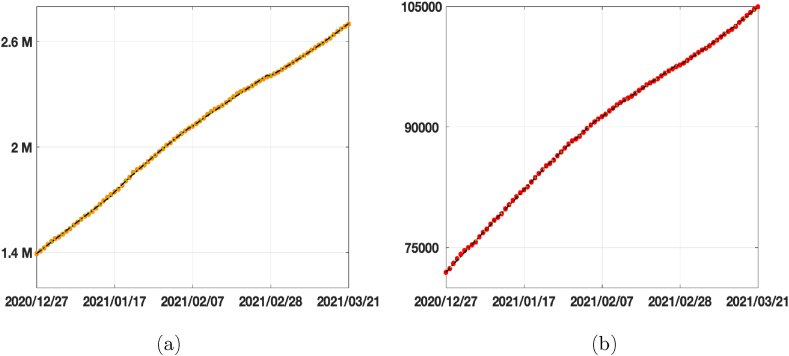
In Fig. 5 (a) and (b) we plot the calibrated functions of infected and the difference between the SEIRDV_exp and SEIRDV_pwl results. In Fig. 6 (a) and (b) the recovered and dead calibrated functions, together with the corresponding data, are reported. We can appreciate the good quality of data-fit of SEIRDV_pwl and SEIRDV_pwe.

Fig. 5.

Calibration results on infected compartment. (a) Data from 2020/12/27 until 2021/03/21 (magenta circles), SEIRDV_pwl calibration (black dashed line), SEIRDV_pwe calibration (green continuous line). (b) Difference between SEIRDV_pwe and SEIRDV_pwl (red circles).

Fig. 6.

Calibration results. (a) Recovered compartment. Data from 2020/12/27 until 2021/03/21 (orange circles), SEIRDV_pwl calibration (black dashed line), SEIRDV_pwe calibration (green continuous line). (b) Dead compartment. Data from 2020/12/27 until 2021/03/21 (cyan circles), SEIRDV_pwl calibration (black dashed line), SEIRDV_pwe calibration (green continuous line).

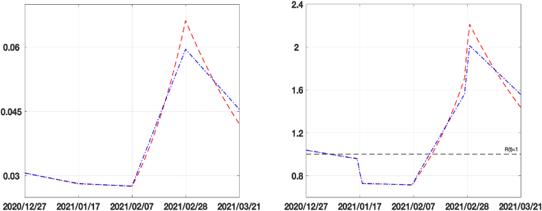
In Fig. 7 we plot the values of both the infection rate function β(t) (on the left) and the reproduction number function R_t(t) (on the right) computed as follows:

$$R_t=\frac{\beta (t)}{\widehat{\gamma }(t)},\widehat{\gamma }(t)=\left\{\begin{array}{cc}{\gamma }_k& t_{k-1}<t<t_k,1<k<p\\ ({\gamma }_k+{\gamma }_{k-1})/2& t=t_k,1<k<p\\ {\gamma }_1& t=t_1\\ {\gamma }_p& t=t_p\end{array}\right)$$ (7)

obtained by extending (A.2) to time dependent parameters β and γ.

Fig. 7.

Forcing β functions (on the left) and Reproduction index R_t (on the right) for SEIRDV_pwl (blue dash-dotted line) and SEIRDV_exp (red dashed line) models.

We observe in Fig. 7 that the red line relative to the exponential model changes more rapidly than that of the linear model when the epidemic spread increases (Δ₃ and Δ₄ intervals). To analyse the behaviour of the infection rate in the considered sub-intervals, we average the values of the calibrated function β(t), represented in Fig. 7 (a), on the intervals [Δ₁, Δ₂], getting 0.0287 for both the methods, and in the period [Δ₃, Δ₄] obtaining 0.0478 and 0.0483 for SEIRDV_pwl SEIRDV_pwe, respectively. These values show that both methods capture the increase of the infection rate that causes the growth of the epidemic curve in Fig. 5(a) in the interval [Δ₃, Δ₄]. Moreover, the decreasing values of β(t) and R_t in the interval Δ₄ (Fig. 7) suggest that the end of epidemic growth could be close, as soon as R_t becomes less than one.

We now discuss the parameters computed in the calibration step and reported in Table 2. Concerning the incubation rate α, both models report a decreasing behaviour in the period Δ₁ − Δ₄. It corresponds to an incubation period between 1.1 and 4.6 days.

Table 2.

Parameters α, γ, η calibrated in the different time intervals (6).

parameter	model	Δ1	Δ2	Δ3	Δ4	mean
α	SEIRDV_pwl	0.8762	0.4286	0.3045	0.2461	0.4638
	SEIRDV_pwe	0.8762	0.4260	0.3231	0.2188	0.4610
γ	SEIRDV_pwl	0.0295	0.0386	0.0371	0.0292	0.0336
	SEIRDV_pwe	0.0295	0.0386	0.0372	0.0293	0.0336
η	SEIRDV_pwl	0.0290	0.0238	0.0216	0.0238	0.0246
	SEIRDV_pwe	0.0290	0.0238	0.0216	0.0238	0.0246

The removal rate γ is very similar for both methods and gives the following removal periods: 34 d(Δ₁), 25.9 d(Δ₂), 26.9 d(Δ₃), 34.2 d(Δ₄) producing the average removal period of 30.3 d.

Regarding the parameter η, we observe that the average value 2.5% obtained by both models slightly underestimates the reference value 3%, reported by Johns Hopkins University Coronavirus Resource Center, https://coronavirus.jhu.edu/data/mortality.

4. Prediction

We use SEIRDV to predict the future behaviour of the disease evolution in short-medium m-days interval [T, T_m], with T_m = T + m.

Writing the last equation of the SEIRDV model (A.1) as:

$$V^{\prime }=\mathcal{U}$$

we obtain the vaccination rate ν_p as the ratio between $\mathcal{U}$ and S.

In this paper we have adopted the following two strategies for prediction.

• 1.We set in (A.1) the parameters Θ_p = (α_p, β_p, γ_p, η_p, ν_p) computed in the last calibration interval Δ_p and we run the model over a unique time interval [T, T_m]. In our simulations we use both the SEIRDV_pwl and SEIRDV_pwe proposed approaches.
• 2.We set in (A.1) the parameters Θ_σ = (α_p, β_p, γ_p, η_p, σ ⋅ ν_p), with σ > 1, to simulate an increased vaccination rate. We compute also in this case the prediction using both the linear and exponential β functions.

4.1. Results of prediction on national data

In this paragraph, we apply the calibrated SEIRDV_pwl and SEIRDV_pwe to make predictions. To test the forecast reliability, we compute a prediction in the interval Δ₅ = [2021/03/21, 2021/04/20] using the data available in that period to measure the precision of our forecast in terms of the Infected peak time and value.

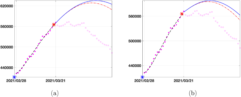
In Fig. 8 we show the predicted curve for infected population. With the red dashed curve we plot the prediction obtained by using the first strategy described, i.e. using the values of all the parameters calibrated in Δ₄. With the continuous blue line, we plot the prediction obtained by considering the first strategy for all the parameters except β(t), which is now set as the function interpolating the curve between the blue and red star (representing the infection rate calibrated in 2021/02/28 and 2021/03/21, respectively). Comparing the prediction curves relative to SEIRDV_pwl (Fig. 8 (a)) and SEIRDV_pwe (Fig. 8 (b)) with the epidemic data represented by magenta empty circles we can see that the exponential model is more accurate.

Fig. 8.

Prediction for the Infected compartment in Italy from 2021/03/22 to 2021/04/20. Data (magenta circles), prediction with β(t) calibrated in the last interval Δ₄ (red dashed line) and prediction with β(t) interpolating the values of β in red and blue stars (blue continuous line). (a) SEIRDV_pwl (b) SEIRDV_pwe.

We highlight that the reported forecast refers to the vaccination rate ν = 0.0018. From Table 3 we can see that the peak of infected people is reached on 2021/04/09 and 2021/04/03 with SEIRD_pwl and SEIRD_pwe, respectively. Comparing to the data, the SEIRD_pwe prevision is more accurate.

Table 3.

Results of the prediction experiment in Italy obtained with different vaccination rates: number of Infected people and day of the peak for SEIRDV_pwl and SEIRDV_pwe. The peak of available data is on 2021/03/28 with 573235 Infected people.

vaccination rate	administration	SEIRDV_pwl		SEIRDV_pwe
	per day	#(infected)	peak day	#(infected)	peak day
0.0018	108215	628504	09/04/21	594604	03/04/21
0.0045	270537	622139	07/04/21	592549	02/04/21
0.0072	534288	617322	06/04/21	590882	01/04/21

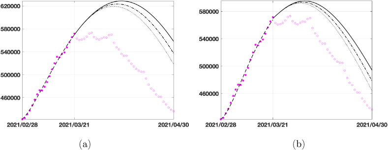
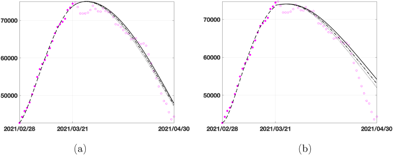
In the second and third lines of the table, we report the number of infected in the peak day together with the date of peak if we suppose to increase the vaccination rate. Graphically, the behaviour of infected is plotted in Fig. 9, where we represent the predictions given by the two models in 40 days using the vaccination rates in Table 3. Comparing the two models, we see that the SEIRDV_pwe gives the more realistic prediction.

Fig. 9.

40 days prediction for the infected compartment in Italy by considering different vaccination rates ν = 0.0018 (dark continuous line), ν = 0.0045 (dark dashed-dotted line) and ν = 0.0072 (dark dotted line): (a) SEIRDV_pwl, (b) SEIRDV_pwe.

4.2. Results of prediction on regional data

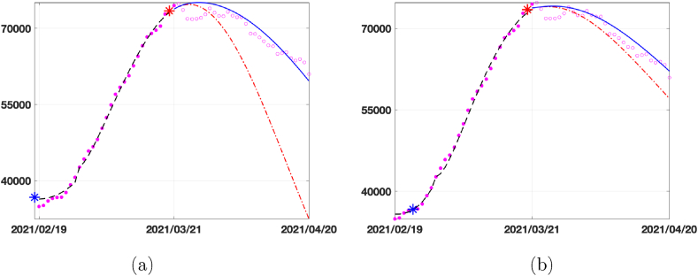
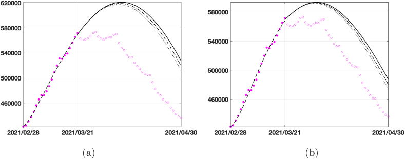
Finally, we present the prediction obtained using more homogeneous and smaller-scale data acquired in the Emilia-Romagna region after performing the calibration on the same sub-intervals as in (6). In Fig. 10 we plot the prediction obtained with the same procedure as in Fig. 8. Differently to what happens for the Italian case, in the linear model (Fig. 10 (a)) the prediction obtained with the red curve is entirely inaccurate, whereas for the exponential model (Fig. 10 (b)) the red and blue lines define a region containing the infected data. Therefore, SEIRDV_pwe can be used to make reliable predictions with both strategies. Finally, in Fig. 11 we show the results for increasing vaccination rates, as done in Fig. 9 for the national data. The SEIRDV_pwl forecasts are now closer to the infected data compared to SEIRDV_pwe, differently from what happened in the national case.

Fig. 10.

Prediction for the infected compartment in Emilia-Romagna from 2021/03/22 to 2021/04/20. Data (magenta circles), prediction with β(t) interpolating the values of β between the red and blue stars (blue continuous line), prediction with β(t) calibrated in the last interval Δ₄. (a) SEIRDV_pwl (b) SEIRDV_pwe.

Fig. 11.

40 days prediction for the Infected compartment in Emilia-Romagna by considering different vaccination rates v = 0.0018 (dark continuous line), v = 0.0045 (dark dashed-dotted line) and v = 0.0072 (dark dotted line): (a) SEIRDV_pwl, (b) SEIRDV_pwe.

4.3. Towards the 80% vaccination

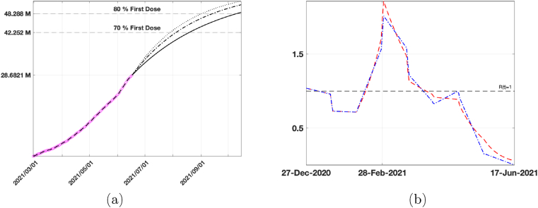
In this experiment we extend the calibration period to the present date (2021/06/12) (using L = 21 as in the previous experiments and p = 8) and run the simulations to forecast the time at which 70%–80% population has received the first vaccine dose. As already observed, the two models have a very similar behaviour in the calibration phase and this behaviour is confirmed also by the forecast data reported in Table 4. The increase of 60% in the vaccination rate causes a reduction of about twenty days to obtain 70% vaccinated population and about one month for 80%. We report in Fig. 12(a) the vaccination data (pink circles), the fitted vaccinated population (black dashed line), together with the forecasts obtained with the calibrated vaccination rate (black continuous line) and with an increased vaccination rate 30% (dot dashed line) and 60% (dotted line), computed by SEIRDV_pwe. We highlight with dashed lines the values of vaccinated individuals corresponding to 70% and 80% of the whole population.

Table 4.

Results of the prediction experiment in Italy obtained by the vaccination rate (first row) calibrated on 17/06/2021 and with a 30% and 60% increase. Dates at which a single vaccine dose is given to 70%–80% people.

vaccination rates	administration per day	SEIRDV_pwl		SEIRDV_pwe
		70%	80%	70%	80%
0.0109	657156	19/08/21	11/10/21	19/08/21	11/10/21
0.0142	854303	05/08/21	14/09/21	05/08/21	14/09/21
0.0163	985735	29/07/21	02/09/21	29/07/21	02/09/21

Fig. 12.

(a) Vaccination data (pink circles), fitted Vaccinated (black dashed line), forecast obtained by SEIRDV_pwe considering the calibrated vaccination rate (black continuous line), an increase of 30% (dot dashed line) and 60% (dotted line) of vaccination rate . (b) Reproduction number R_t obtained by both SEIRDV_pwl (blue dash dot line) and SEIRDV_pwe (red dashed line) at the fitted vaccination rates.

In Fig. 12(b) we represent the reproduction number R_t of both SEIRDV_pwl and SEIRDV_pwe which confirms the positive effect of the current vaccination campaign.

5. Conclusions

We have proposed two switched SEIRDV compartmental models, each involving six populations (susceptibles, exposed, infected, recovered, dead and vaccinated) to analyse COVID-19 spread from the beginning of the vaccination campaign in Italy. We have considered as vaccinated people who have received one dose of vaccine in Italy. The two schemes differ in the forcing time-dependent infection rate function. We have calibrated the models from data in the first three months of the vaccination campaign with switch time intervals of about 20 days. Thirty days forecasts are discussed by changing the infection and the vaccination rates according to two different strategies.

We summarize here the primary outcomes. Both models compute very similar parameters which fit the literature ranges. The data fit is very faithful for all the considered compartments with a relative residual value less than 1%. The infection rate function in SEIRDV_pwe changes more rapidly when the epidemic spread increases. The thirty days forecasts, from mid-March to mid-April 2021, show that the SEIRDV_pwe predicts the infected peak and values more accurately than SEIRDV_pwl, even if both methods predict the peak day a few days later than the observed data.

Using regional data from Emilia-Romagna, the 30 days prediction is more accurate and SEIRDV_pwe outperforms SEIRDV_pwl.

Finally, we applied the model calibrated to 2021/06/17 to predict when 70%–80% of the population has received one vaccine dose. At the present vaccination rate, 80% immunization is reached on 2021/10/11, whereas with an increase of 60% (best scenario) it is reached on 2021/09/02.

The experiment of the preliminary extension of the proposed model accounting for the limited duration of vaccine efficacy, shows that different vaccination rates give very similar infected curves. Hence, in the initial phase of the vaccination campaign, the epidemic evolution was not sensible to the number of vaccines administered.

Future studies and extensions of the proposed model will also include the possibility of re-infection and the distinction between one and two vaccination doses. We believe that such an extension, together with a more detailed population age structure, will give its decisive contribution in the autumn-winter epidemic spread.

Declaration of competing interest

The authors declare that they have no known competing financial interests or personal relationships that could have appeared to influence the work reported in this paper.

Handling Editor: Dr Lou Yijun

Appendix A. The SEIRDV model with constant parameters

The SEIRDV model characterized by constant parameters is obtained from the SEIRD model (Piccolomini and Zama, 2020) by adding the new compartment V representing the vaccinated population. The following differential system represents the populations’ dynamics:

$$\begin{array}{cc}& S^{\prime }=-\frac{\beta }{N}SI-\nu S,\\ & E^{\prime }=\frac{\beta }{N}SI-\alpha E\\ & I^{\prime }=\alpha E-\gamma I\\ & R^{\prime }=\gamma (1-\eta )I\\ & D^{\prime }=\gamma \eta I\\ & V^{\prime }=\nu S\end{array}$$ (A.1)

where the total population, assumed of constant size N, is subdivided into six compartments: susceptible (S), exposed (E), infected (I), recovered (R), dead (D) and vaccinated (V). System (A.1) is solved starting from an initial time t = t₀ where the values S(t₀), E(t₀), I(t₀), R(t₀), D(t₀), V(t₀) are assigned on the basis of the available data and integrated up to a final time T. The parameter β ≥ 0 represents the infection rate, accounting for the susceptible people infected by infectious people. Thus, its value is related to the number of contacts between susceptible and infected. Standard models, as well as our SEIRDV, assume this relationship to be linear. A reference value β₀ = 0.02 to be used as starting guess in our model has been obtained by running switched forced SEIRD (Piccolomini and Zama, 2020) up to December 2019.

The parameter α > 0 represents the incubation rate for the transition from exposed to infected states. Such value relates to the incubation period A_I as follows: A_I = 1/α. The average incubation for COVID-19 ranges from 2 to 14 days (d) (see https://www.worldometers.info/coronavirus/coronavirus-incubation-period/). According to (Lauer et al., 2020), more than 97 percent of people who contract SARS-CoV-2 show symptoms within 11.5 days of exposure. Recently a comparative study assesses the incubation period of COVID-19 around 6.5 days (Alene et al., 2021). The cited studies assess the value of α in the interval [0.14, 0.5]. Hence we consider α₀ = 1/6 as starting guess in our model.

The parameter γ > 0 representing the removal rate relates to the average infectious period T_I as γ = 1/T_I. At the beginning of the COVID-19 outbreak, an average value T_I ≃ 20 d has been measured (Zhou et al., 2020), hence γ ∈ [0.03, 0.1]. The starting guess used in this case is γ₀ = 1/20.

After the period T_I, the infected people split into recovered and dead with weights 1 − η and η, respectively (0 ≤ η ≤ 1). Hence the parameter η represents the fraction of the removed individuals who die and its value depends on environmental situations that change over time, such as the population age, the virus spread, medical care availability and treatments. We use as starting guess for this value is η₀ = 0.001. Finally, the parameter ν > 0 represents the vaccination rate. Its value is particularly useful in the prediction phase to obtain different scenarios.

Important information about the epidemic development is obtained from the number of infection cases generated from a single infectious individual, i.e. the basic reproduction number R₀, defined as follows (see details in AppendixA.1):

$$R_0=\frac{\beta }{\gamma }.$$ (A.2)

It is well known that the epidemic occurs when R₀ > 1; however, this information refers to the initial stage, assuming that the entire population is susceptible. In the case of COVID-19, estimates of R₀ in the interval [1.5, 6.68] were obtained during the first months of 2020 (Achaiah et al., 2020).

Appendix A.1.

Concerning the analysis of stability and equilibrium solutions of a compartmental model with different vaccination policies, please refer to (Etxeberria-Etxaniz, Alonso-Quesada, & De la Sen, 2020) and references therein. Using the relation N = S(t) + E(t) + I(t) + R(t) + D(t) + V(t), we can eliminate the last equation in (A.1) and define a disease free equilibrium (S∗, E∗, I∗, R∗, D∗), with I∗ = E∗ = R∗ = D∗ = 0. Following the next generation matrix approach (van den DriesscheJames, 2002; Brauer, Castillo-Chavez, & Castillo-Chavez, 2012), we compute the basic Reproduction Number R₀, defined as the number of secondary cases generated by a single infected. Let X = [E,I]^T be the state at infection of system (A.1), then the exposed and infected equations can be written as: X′ = F(X) + W(X) where

$$F(X)=\left(\begin{array}{c}\beta SI/N\\ 0\end{array}\right),W(X)=\left(\begin{array}{c}\alpha E\\ -\alpha E+\gamma I\end{array}\right)$$

The Jacobian matrices of F and W at the disease free equilibrium are:

$$\mathbf{F}=\left(\begin{array}{cc}0& \beta S^{\ast }/N\\ 0& 0\end{array}\right),\mathbf{W}=\left(\begin{array}{cc}\alpha & 0\\ -\alpha & \gamma \end{array}\right)$$

According to (van den DriesscheJames, 2002) the basic reproduction number R₀ is the maximum eigenvalue of the next generation matrix NGM = FW⁻¹, i.e.

$$NGM=\mathbf{F}\left(\begin{array}{cc}1/\alpha & 0\\ 1/\gamma & 1/\gamma \end{array}\right)=\frac{S^{\ast }\beta }{N\gamma }\left(\begin{array}{cc}1& 1\\ 0& 0\end{array}\right)$$

In the assumption that at disease free state S∗ = N we obtain (A.2). We note that it coincides with the R₀ value of a standard SEIR model (Keeling & Rohani, 2011).

Appendix B. Model extension considering vaccination efficacy

Since it us known that the vaccine efficacy is not complete, we propose here a preliminary experiment extending the SEIRDV model in (4) as suggested in (Cai et al., 2018). The extended model is represented by the following equations:

$$\begin{array}{cc}& S^{\prime }=-\frac{\beta }{N}SI-\mathcal{U},\\ & V^{\prime }=\mathcal{U}-\rho \frac{\beta }{N}VI\\ & E^{\prime }=\frac{\beta }{N}SI-\alpha E+\rho \frac{\beta }{N}VI\\ & I^{\prime }=\alpha E-\gamma I\\ & R^{\prime }=\gamma (1-\eta )I\\ & D^{\prime }=\gamma \eta I\end{array}$$ (B.1)

where the parameter ρ ∈ [0, 1] measures the vaccine efficacy. We observe that if ρ = 0 the vaccine is perfectly effective and the model coincides with (4).

We present some experiments where we change the vaccine efficacy according to the values reported in (Lopez Bernal et al., 2021) in the case of a single dose. In particular, using the vaccine efficacy VC = 48.7% against Alpha variant proposed in (Lopez Bernal et al., 2021), we set ρ = 1–0.487 = 0.513, since the Alpha variant was widely diffused in Italy at the time of our experiments.

Fig. B.13.

40 days prediction for the infected compartment in Italy by considering different vaccination rates v = 0.0018 (dark continuous line), v = 0.0045 (dark dashed-dotted line) and v = 0.0072 (dark dotted line): (a) SEIRDV_pwl, (b) SEIRDV_pwe.

Fig. 9 represents the infected populations obtained by the model (B.1) with the linear and exponential infection rates calibrated as in section (3.2) with the vaccination rates given in Table 4. We observe that the decreased vaccine efficacy does not affect the infected curve behaviour and the peak day. On the contrary, the reduced efficacy of the vaccine causes the infected curves at different vaccination rates to be closer each other (compared to Fig. 9). Comparing the two models, we notice that the exponential model is closer to the infected data and the number of infected people is significantly lower.

References

- Achaiah N.C., Subbarajasetty S.B., Shetty R.M. R0 and re of covid-19: Can we predict when the pandemic outbreak will be contained? Indian Journal of Critical Care Medicine: Peer-Reviewed, Official Publication of Indian Society of Critical Care Medicine. 2020;24(11):1125. doi: 10.5005/jp-journals-10071-23649. [DOI] [PMC free article] [PubMed] [Google Scholar]
- Acuña-Zegarra M.A., Díaz-Infante S., Baca-Carrasco D., Liceaga D.O. Mathematical Biosciences; 2021. Covid-19 optimal vaccination policies: A modeling study on efficacy, natural and vaccine-induced immunity responses. [DOI] [PMC free article] [PubMed] [Google Scholar]
- Alene M., Yismaw L., Assemie M.A., Ketema D.B., Gietaneh W., Birhan T.Y. Serial interval and incubation period of covid-19: A systematic review and meta-analysis. BMC Infectious Diseases. 2021;21(1):1–9. doi: 10.1186/s12879-021-05950-x. [DOI] [PMC free article] [PubMed] [Google Scholar]
- Brauer F., Castillo-Chavez C., Castillo-Chavez C. ume 2. Springer; 2012. (Mathematical models in population biology and epidemiology). [Google Scholar]
- Burnham K.P., Anderson D.R. Multimodel inference: Understanding aic and bic in model selection. Sociological Methods & Research. 2004;33(2):261–304. [Google Scholar]
- Cai L.-M., Li Z., Song X. Global analysis of an epidemic model with vaccination. Journal of Applied Mathematics and Computing. 2018;57(1):605–628. doi: 10.1007/s12190-017-1124-1. [DOI] [PMC free article] [PubMed] [Google Scholar]
- Chen Q., Allot A., Lu Z. LitCovid: An open database of COVID-19 literature. Nucleic Acids Research. 2020;49(D1):11. doi: 10.1093/nar/gkaa952. D1534–D1540. [DOI] [PMC free article] [PubMed] [Google Scholar]
- van den Driessche P., James W. Reproduction numbers and sub-threshold endemic equilibria for compartmental models of disease transmission. Mathematical Biosciences. 2002;180(1):29–48. doi: 10.1016/s0025-5564(02)00108-6. [DOI] [PubMed] [Google Scholar]
- El Koufi Amine, Bennar A., Yousfi N. Dynamics behaviors of a hybrid switching epidemic model with levy noise. Applied Mathematics. 2021;15(2):131–142. [Google Scholar]
- Etxeberria-Etxaniz M., Alonso-Quesada S., De la Sen M. On an seir epidemic model with vaccination of newborns and periodic impulsive vaccination with eventual on-line adapted vaccination strategies to the varying levels of the susceptible subpopulation. Applied Sciences. 2020;10(22):8296. [Google Scholar]
- Friji H., Hamadi R., Ghazzai H., Besbes H., Massoud Y. A generalized mechanistic model for assessing and forecasting the spread of the covid-19 pandemic. IEEE Access. 2021;9:13266–13285. doi: 10.1109/ACCESS.2021.3051929. [DOI] [PMC free article] [PubMed] [Google Scholar]
- Giordano G., Colaneri M., Di Filippo A., Franco B., Bolzern P., De Nicolao G., Sacchi P., Colaneri P., Bruno R. Modeling vaccination rollouts, sars-cov-2 variants and the requirement for non-pharmaceutical interventions in Italy. Nature Medicine. 2021:1–6. doi: 10.1038/s41591-021-01334-5. [DOI] [PMC free article] [PubMed] [Google Scholar]
- Goebel R., Sanfelice R.G., Teel A.R. Princeton University Press; 2012. Hybrid dynamical systems. [Google Scholar]
- Keeling M.J., Rohani P. Princeton university press; 2011. Modeling infectious diseases in humans and animals. [Google Scholar]
- Kermack W.O., McKendrick A.G. Vol. A. 1927. A contribution to the mathematical theory of epidemics; pp. 700–721. (Proceedings of the royal society of London). [Google Scholar]
- Lauer S.A., Grantz K.H., Bi Q., Jones F.K., Zheng Q., Meredith H.R., Azman A.S., Reich N.G., Lessler J. The incubation period of coronavirus disease 2019 (covid-19) from publicly reported confirmed cases: Estimation and application. Annals of Internal Medicine. 2020;172(9):577–582. doi: 10.7326/M20-0504. [DOI] [PMC free article] [PubMed] [Google Scholar]
- Liu X., Stechlinski P. Infectious disease models with time-varying parameters and general nonlinear incidence rate. Applied Mathematical Modelling. 2012;36(5):1974–1994. [Google Scholar]
- Lopez Bernal J., Andrews N., Gower C., Gallagher E., Simmons R., Simon T., Julia Stowe, Tessier E., Groves N., Gavin D., et al. New England Journal of Medicine; 2021. Effectiveness of covid-19 vaccines against the b. 1.617. 2 (delta) variant. [DOI] [PMC free article] [PubMed] [Google Scholar]
- Maher Ala’raj, Majdalawieh M., Nizamuddin N. Modeling and forecasting of covid-19 using a hybrid dynamic model based on seird with arima corrections. Infectious Disease Modelling. 2021;6:98–111. doi: 10.1016/j.idm.2020.11.007. [DOI] [PMC free article] [PubMed] [Google Scholar]
- Morettini M., Sbrollini A., Marcantoni I., Burattini L. Covid-19 in Italy: Dataset of the Italian civil protection department. Data in brief. 2020;30:105526. doi: 10.1016/j.dib.2020.105526. [DOI] [PMC free article] [PubMed] [Google Scholar]
- Parolini N., Dede’ L., Antonietti P., Ardenghi G., Manzoni A., Miglio E., Andrea Pugliese, Verani M., Quarteroni A. 2021. Suihter: A new mathematical model for covid-19. Application to the analysis of the second epidemic outbreak in Italy. [DOI] [PMC free article] [PubMed] [Google Scholar]
- Piccolomini Elena Loli, Zama F. Monitoring Italian covid-19 spread by a forced seird model. PLoS One. 08 2020;15(8):1–17. doi: 10.1371/journal.pone.0237417. [DOI] [PMC free article] [PubMed] [Google Scholar]
- Rachaniotis N.P., Dasaklis T.K., Fotopoulos F., Tinios P. A two-phase stochastic dynamic model for covid-19 mid-term policy recommendations in Greece: A pathway towards mass vaccination. International Journal of Environmental Research and Public Health. 2021;18(5):2497. doi: 10.3390/ijerph18052497. [DOI] [PMC free article] [PubMed] [Google Scholar]
- Roy S., Dutta R., Ghosh P. Optimal time-varying vaccine allocation amid pandemics with uncertain immunity ratios. IEEE Access. 2021;9:15110–15121. [Google Scholar]
- Zhou F., Ting Y., Du R., Fan G., Liu Y., Liu Z., Xiang J., Wang Y., Song B., Gu X., Guan L., Yuan W., Li H., Wu X., Xu J., Tu S., Zhang Y., Chen H., Cao B. Clinical course and risk factors for mortality of adult inpatients with covid-19 in wuhan, China: A retrospective cohort study. Lancet. 2020 doi: 10.1016/S0140-6736(20)30566-3. [DOI] [PMC free article] [PubMed] [Google Scholar]
- Zhu J., Gallego B. Evolution of disease transmission during the covid-19 pandemic: Patterns and determinants. Scientific Reports. 2021;11(1):1–9. doi: 10.1038/s41598-021-90347-8. [DOI] [PMC free article] [PubMed] [Google Scholar]