Fully Automated Multi-Organ Segmentation of Female Pelvic Magnetic Resonance Images with Coarse-to-Fine Convolutional Neural Network

Abstract

Purpose:

Brachytherapy (BT) combined with external beam radiotherapy (EBRT) is the standard treatment for cervical cancer and has been shown to improve overall survival rates compared to EBRT only. Magnetic resonance (MR) imaging is used for radiotherapy (RT) planning and image guidance due to its excellent soft tissue image contrast. Rapid and accurate segmentation of organs at risk (OAR) is a crucial step in MR image-guided RT. In this paper, we propose a fully automated two-step convolutional neural network (CNN) approach to delineate multiple OARs from T2-weighted (T2W) MR images.

Methods:

We employ a coarse-to-fine segmentation strategy. The coarse segmentation step first identifies the approximate boundary of each organ of interest and crops the MR volume around the centroid of organ-specific region of interest (ROI). The cropped ROI volumes are then fed to organ-specific fine segmentation networks to produce detailed segmentation of each organ. A three-dimensional (3-D) U-Net is trained to perform the coarse segmentation. For the fine segmentation, a 3-D Dense U-Net is employed in which a modified 3-D dense block (DB) is incorporated into the 3-D U-Net-like network to acquire inter and intra-slice features and improve information flow while reducing computational complexity. Two sets of T2W MR images (221 cases for MR1 and 62 for MR2) were taken with slightly different imaging parameters and used for our network training and test. The network was first trained on MR1 which was a larger sample set. The trained model was then transferred to the MR2 domain via a fine-tuning approach. Active learning strategy was utilized for selecting the most valuable data from MR2 to be included in the adaptation via transfer learning.

Results:

The proposed method was tested on 20 MR1 and 32 MR2 test sets. Mean±SD dice similarity coefficients (DSCs) are 0.93±0.04, 0.87±0.03, and 0.80±0.10 on MR1 and 0.94±0.05, 0.88±0.04, and 0.80±0.05 on MR2 for bladder, rectum, and sigmoid, respectively. Hausdorff distances (95^th percentile) are 4.18±0.52, 2.54±0.41, and 5.03±1.31 mm on MR1 and 2.89±0.33, 2.24±0.40, and 3.28±1.08 mm on MR2, respectively. The performance of our method is superior to other state-of-the-art segmentation methods.

Conclusions:

We proposed a two-step CNN approach for fully automated segmentation of female pelvic MR bladder, rectum, and sigmoid from T2W MR volume. Our experimental results demonstrate that the developed method is accurate, fast, and reproducible, and outperforms alternative state-of-the-art methods for OAR segmentation significantly (p<0.05).

1. INTRODUCTION

Over 600,000 women are diagnosed with cervical cancer each year worldwide, which is the fourth most commonly occurring cancer in women^1,2. For curative management of locally advanced disease, external beam radiation therapy (EBRT) followed by brachytherapy (BT) is performed. BT involves placing radiation sources inside the target tumor region through temporary catheters to destroy the tumor. Research demonstrates that cervical cancer BT improves survival rates by 30–40% over EBRT alone³. Currently, computed tomography (CT) is used as the primary image modality for both EBRT planning and applicator localization in BT. However, due to the lack of sufficient soft tissue contrast in CT, it is highly desirable to utilize MRI to better visualize the target tumor and organs at risk (OARs) in order to improve the treatment accuracy and outcome. Once RT planning images are obtained, the first step is to contour the target tumor and OARs, which is typically done manually by the attending radiation oncologist and therefore very time-consuming.

In this study, we propose a fully automated coarse-to-fine segmentation approach using convolutional neural networks (CNNs) to accurately and efficiently segment OARs in female pelvic MR images. While CT-based pelvic OAR segmentation has been actively studied^4–8 there are few studies of automatic segmentation of pelvic MR images, with most existing studies focused on male pelvic OARs for prostate cancer diagnosis and treatment⁹. Segmenting OARs in MR images may be considered easier than CT given superior soft tissue image contrast. However, automated OAR segmentation in MR images is challenging because, unlike CT, MR image intensity is not standardized and therefore is more variable between patients and even within the same patient. Furthermore, there are much more image contexts shown in MR images that are often similar to those of the target organ to be segmented, confusing the segmentation algorithm. Therefore, automatic segmentation often performs poorly with MRI than CT^4,5. In addition, organs with variable and complex shapes and textures are more challenging to accurately segment, especially without carefully considering their whole three-dimensional (3-D) anatomy. Figure 1 shows an example of manual segmentation of the sigmoid in T2-weighted (T2W) MR images. The sigmoid appearance is significantly variable not only in axial views but also across adjacent slices. Moreover, neighboring tissues share the same contextual information with the sigmoid.

Fig. 1.

Example of manual sigmoid segmentation in T2W MRI shown at four adjacent axial slices.

In past decades, many automatic segmentation methods were proposed^10–13 among which deep learning (DL)-based approaches are widely used outperforming all prior methods. Although the potential of DL-based segmentation of pelvic structures in MR images has been explored, there are few studies of female pelvic image segmentation. Nie et al.¹⁴ introduced a spatially-varying stochastic residual adversarial network in which a stochastic residual unit was used in a plain convolutional layer in the fully convolutional networks (FCN) to segment the bladder, prostate, and rectum in MR images. A dilated convolution, spatially-varying convolutional layer, and an adversarial network have been applied to the suggested network to further improve the performance. Yu et al.¹⁵ introduced a method for prostate segmentation in which a residual learning module is incorporated into U-Net. Zabihollahy et al.^16–17 used ensemble learning to segment the prostate and its transition and peripheral zones from T2W and apparent diffusion coefficient (ADC) maps of MRI for tumor localization. Zhu et al.¹⁸ utilized a deep supervision mechanism to train a U-Net-like network to segment the prostate from MRI. Liu et al.¹⁹ employed an FCN with feature pyramid attention to perform prostate segmentation. Although all of these methods achieved reasonable results, segmentation was based on two-dimensional (2-D) slice images, i.e., 3-D segmentation was generated by stacking 2-D segmentations. Therefore, inter-slice information was ignored, limiting the performance.

We employ a 3-D CNN to effectively probe inter-slice features and 3-D contexts for accurate OAR segmentation. Li et al.²⁰ demonstrated that hybrid densely connected U-Net (2-D DenseUNet) outperformed state-of-the-art methods for liver tumor segmentation from CT images. We built our method upon this work and improved the method by using a 3-D dense block (DB) as the second convolutional layer in the contracting and expanding paths of the 3-D U-Net-like architecture to mitigate learning redundant features and enhance information flow. Our method has two main differences with Densely Connected Convolutional Networks (DenseNet)²¹; 1) 3-D convolutional layers are used in DBs to preserve volumetric spatial features for better inter-slice context exploration. 2) 3D U-Net-like connections are added to the network with skip connections that enable low-level spatial feature preservation. The introduced network is different from 3-D U-Net as the DB is used as the second convolutional layer in all stages of the contraction-expansion paths. 3-D Dense U-Net strengthens feature propagation by using extra skip connections in DB that concatenate the feature maps of all preceding layers as inputs in all subsequent layers²². To further improve the segmentation accuracy, a coarse-to-fine segmentation strategy is utilized to first identify each organ in MR volume by the coarse segmentation network, crop each organ with added margin, and then feed the cropped volume to the 3-D Dense U-Net to generate a detailed segmentation.

In this study, we obtained two MRI datasets from gynecological cancer patients treated at Johns Hopkins Department of Radiation Oncology. Both sets included T2W sequences but with different imaging parameters. 221 cases were scanned with TR=2600 ms (MR1) and 62 cases with TR=3500 ms (MR2). MR2 has an improved soft-tissue image contrast, therefore is our preferred set to segment OARs. Since the number of data in MR2 is too small, we first trained our network using the MR1 dataset, and then further trained the network with the MR2 dataset through active and transfer learning. Zhou et al.²³ demonstrated that integrating active learning and transfer learning into a single framework enhances CNN’s performance for biomedical image analysis. Therefore, a combination of active learning and transfer learning strategies is adapted in which the trained network (with MR1), hereafter referred to as the baseline network, is employed to select the most valuable samples from MR2 for fine-tuning the network.

The main contributions of this study can be summarised as:

• We developed a 3-D Dense U-Net that combines 3-D U-Net and 3-D DBs to explore the inter and intra-slice context information of MR volume and encourage effective feature propagation through the deep network. Our method differs from the standard 3-D U-Net as the second convolutional layer in the contraction-expansion paths is replaced by modified DBs. In the proposed network, 3-D DBs are used to effectively exploit and distribute 3-D contexts.

• Active learning followed by a transfer learning approach was employed to select the most valuable data for fine-tuning the baseline network. We investigated whether the fine-tuned network trained on relatively small number of training data in MR2 would be able to accurately and robustly segment OARs in MR2 images.

• Our network was trained to segment the bladder, rectum, and sigmoid. We then compared its segmentation performance to standard CNNs as well as other state-of-the-art methods. To our knowledge, this is the first study to automatically segment sigmoid in MR images.

2. MATERIALS AND METHODS

Figure 2 shows the workflow used in our method. We employ a cascaded coarse-to-fine strategy to reduce the computational complexity and more precisely identify the OAR boundaries, which has been used in many medical image segmentation tasks^8,24–26. Siddique et al.²⁷ summarized the benefit and applications of cascaded (or alternatively coarse to fine) network, including cascaded U-Net for multi-organ segmentation. First, a 3-D U-Net is trained to get the coarse segmentation of each organ from which an organ-specific ROI is computed. The original volume is then cropped using the ROI. 3-D Dense U-Net is employed for fine segmentation of each organ from the cropped MRI volume.

Fig. 2.

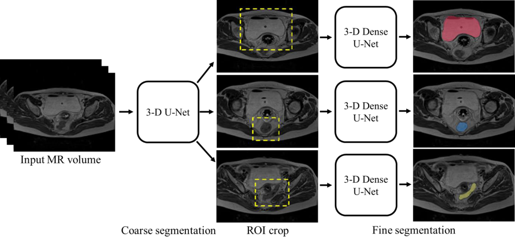
The proposed coarse-to-fine OAR segmentation workflow.

2.A. Datasets

With the approval of the institutional review board, two T2W MR image datasets (221 MR1 and 62 MR2) were collected from a total of 181 patients (note that some patients had more than one MRI scan) who underwent RT at our institution. T2W MR images were obtained as part of a routine RT planning process using the Siemens Espree 1.5T scanner (Siemens Healthineers, Malvern, PA) with a 3-D T2W SPACE (Sampling Perfection with Application-optimized Contrasts using different flip angle Evolution) sequence (TR=2600 ms, TE=95 ms [for MR1] and TR=3500 ms, TE=97 ms [for MR2], and slice thickness=1.60 mm [for both MR1 and MR2]). MR1 images have 640×580×(104–144) voxels with a voxel size of 0.5625×0.5625×1.60 mm³. MR2 images have 320×290×(112–120) voxels with a voxel size of 1.0×1.0×1.6 mm³. The obtained images were manually contoured first by radiation oncology residents followed by review and correction by an expert radiation oncologist specialized in gynecological cancer for RT planning. In this study, we trained and tested the proposed method on the bladder, rectum, and sigmoid. Examples of MR images from two datasets are shown in Fig. 3.

Fig. 3.

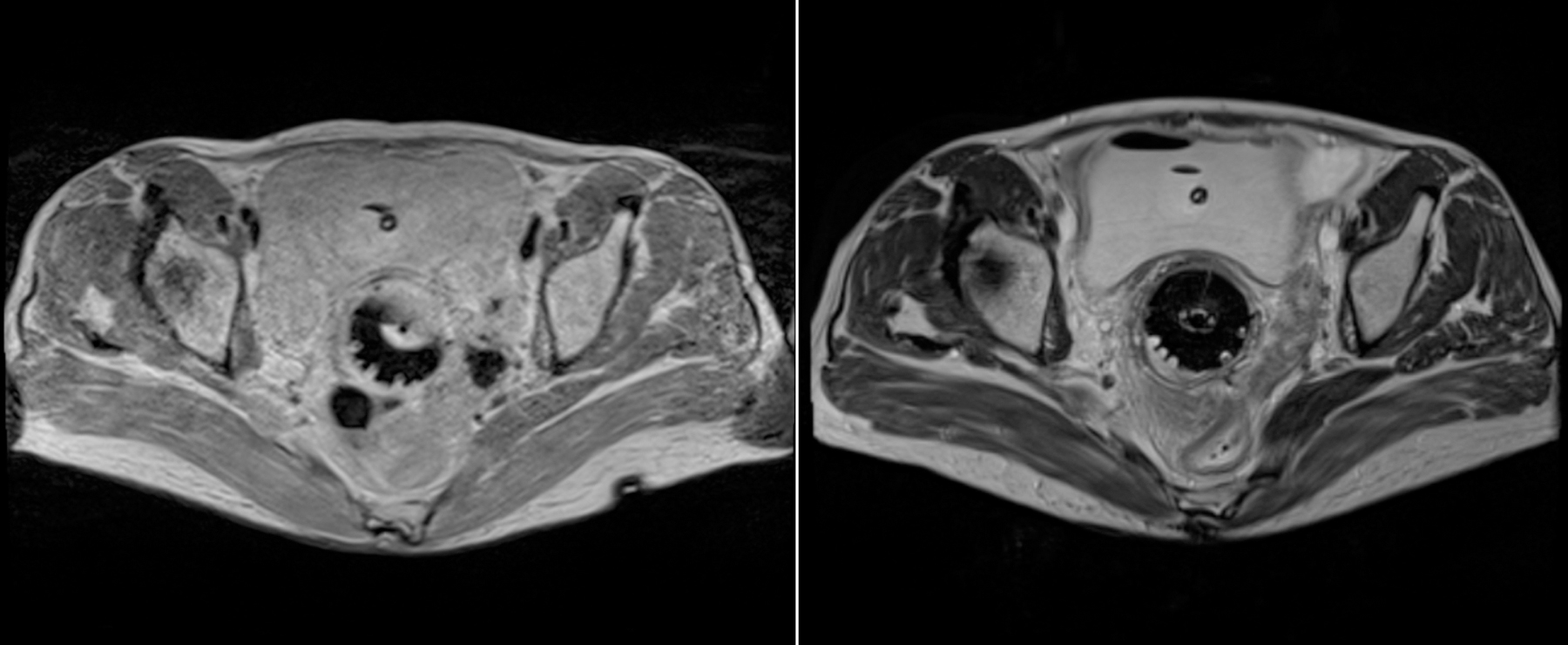
Example (left) MR1 and (right) MR2 images.

2.B. Coarse segmentation

As the original MR volume contains a large background that carries contextual information irrelevant to the target organs, a single multi-label U-Net-based coarse segmentation using a 3-D U-Net is performed to extract the organ-specific ROI from the input MR volume. This step not only improves the segmentation performance by discarding features from the irrelevant background but also reduces the computational complexity by reducing the input volume size.

The 3-D U-Net used for coarse segmentation consists of contraction and expansion paths each with four layers. For the contraction path, the number of kernels is set to 16 in the first layer that doubles at successive layers. The expansion path has a symmetrical architecture of the contraction path. At the final stage, a 1×1×1 convolution followed by the sigmoid activation is applied to all feature maps to generate a probability map. The probability map is then thresholded to produce the binary label map.

2.C. Fine segmentation

Fine segmentation network takes the organ-specific ROI MR volume obtained from the coarse segmentation as input to precisely segment each organ of interest. Organ-specific fine segmentation models are designed using a modified 3-D U-Net with a modified DB. DenseNet, which connects each layer to every other layer in a feed-forward fashion, has been shown to alleviate the vanishing gradient problem, strengthen feature propagation, encourage feature reuse, and substantially reduce the number of parameters compared to traditional CNNs²¹. DenseNet consists of two main building blocks, DB and transition block. In DB, a different connectivity pattern is used where direct connections from any layer to all subsequent layers are introduced. The transition block used between DBs performs convolution and pooling operations. Original DenseNet was designed for the classification task. As we aim to segment OARs, DB is embedded into the encoder-decoder architecture of the 3-D U-Net. This new approach inherits the advantages of both the densely connected path and the U-Net-like connections. The modified DB used in our network is comprised of three layers where the number of feature maps in the first layer is 8 and is multiplied by three in the subsequent layers. In each layer, a 3×3×3 convolution, followed by batch normalization, and a rectified linear unit (ReLU) activation is performed. Although 3-D U-Net with 3-D DB produces a high-level feature representation and spreads it through the network via skip connections, implementing such a deep network is computationally expensive. We, therefore, replaced only the second convolutional layer in each and every stage in contraction-expansion paths of the 3-D U-Net with a modified DB to address this issue. The architecture of the proposed method is shown in Fig. 4.

Fig. 4.

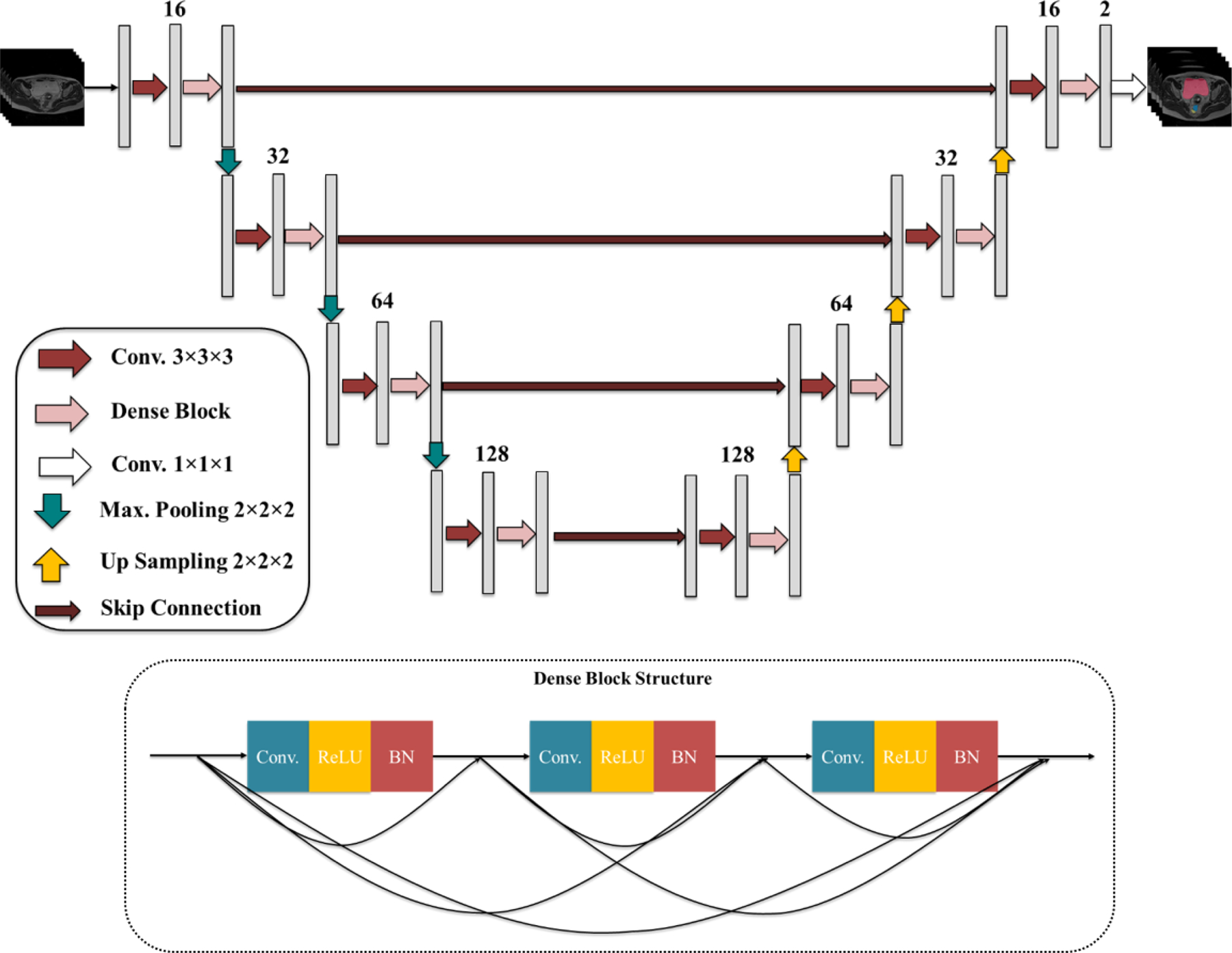
The proposed 3-D Dense U-Net and Dense Block structures.

2.D. Integrated active learning and transfer learning

Transfer learning has been widely used in DL-based medical image processing tasks where collecting a large amount of well-curated data is challenging. Tajbakhsh et al.²⁸ demonstrated that layer-wise fine-tuning a CNN that is pre-trained using a large set of labeled images, for instance, natural images such as in ImageNet, could offer a practical way to reach the best performance for applications with limited available data. However, Raghu et al.²⁹ showed that transfer learning offers little benefit to performance in medical imaging tasks due to fundamental differences in data sizes and features between natural and medical images, and lightweight models can perform comparably to complex networks pre-trained with ImageNet data.

In this study, we use two sets of MR image data; MR1 with 221 cases and MR2 with 62 cases. Therefore, a lightweight model is first trained from scratch using MR images taken with one set of imaging parameters (MR1), and then the learned knowledge is transferred to the new image domain obtained with different imaging parameters (MR2) via layer-wise fine-tuning. Since both MR1 and MR2 use the T2W SPACE sequence with only a few parameter changes, i.e., images are much more similar between MR1 and MR2 than unrelated natural images, the proposed active and transfer learning is preferred to typical transfer learning approaches using more complex networks pre-trained on natural images. Similar to other transfer learning approaches, all layers in the pre-trained baseline network except for the final layer are frozen as the initial layers capture generic features while the later ones focus more on the specific task at hand. Instead of randomly selecting data for fine-tuning, an active learning scheme is used to select the most valuable data from MR2. The criterion for worthy samples is defined as follows. We first take the baseline network trained with MR1 and apply it to MR2 images. The average segmentation accuracy in terms of Dice similarity coefficient (DSC) across all OARs for each patient is calculated. The DSC metric provides a useful indicator of the power of the candidate in improving the performance of the baseline network for OAR segmentation on MR2 images. We considered cases with the lowest DSC as the most valuable samples for fine-tuning the baseline network because they are less predictable by the baseline network. Accordingly, 60% of the data with the lowest DSC are selected for fine-tuning the baseline model.

2.E. Implementation details

Both the coarse and fine segmentation networks were trained using DSC as the similarity metric and optimized using AdaDelta that does not require manual tuning for learning rate and is robust to noisy gradients, differences in CNN architecture, various data modalities, and hyper-parameter selection³⁰.

For MR1, 221 cases obtained from 129 patients were split into 201 (from 122 patients) for training and 20 (from 7 patients) for testing. The training data were augmented via random shift and rotation, yielding 804 volumes. The baseline network was first trained for 300 epochs, and it was observed that the segmentation performance degrades after 200 epochs on the validation set while it improves on the training set. Based on this, the number of epochs for training the baseline networks was set to 200. For coarse segmentation, we first cropped and resampled the original MR volume around the center with a fixed size of 94×94×50 voxels and a voxel size of 3.0×3.0×3.2 mm³. For fine segmentation, three ROI volumes of 96×96×43 (bladder), 75×75×53 (rectum), and 90×90×32 (sigmoid) voxels were extracted from the original MR volume with voxel sizes of 1.5×1.5×3.0 mm³, 1.5×1.5×3.0 mm³, and 2.0×2.0×3.0 mm³, respectively. ROI size of each organ was determined considering the organ size plus margin that is sufficiently large enough not to miss the whole organ. Each ROI volume was downsampled to have the maximum possible resolution to fit within the given GPU memory. Since the sigmoid is more widely distributed in the axial view, we had to use a slightly larger voxel size than the bladder and rectum.

For MR2, 62 cases obtained from 52 patients were split into 30 (from 22 patients) for fine-tuning the baseline network and 32 (from 30 patients) for testing. As the transfer learning approach was adopted for MR2 segmentation, the same image size and resolution as used for MR1 segmentation were used for MR2. For fine-tuning, all layers of the baseline network were frozen except for the final DB layers. We tested the model performance by varying the number of frozen layers, i.e., first freezing the whole layers except for the final DB layer, and gradually unfreezing more layers, and observed that fine-tuning only the final DB layer gives the best segmentation results for all three organs. We believe this is because increasing the number of trainable parameters in the network given the small number of training samples in MR2 (only 30 cases) causes overfitting. Based on these experiments, we chose to fine-tune the last DB layer as the best strategy for knowledge transfer (from MR1) to the new domain (MR2). Thus, the final DB layers were fine-tuned for 50 epochs using the MR2 dataset selected through the active learning process and augmented to 180 using random shift and rotation.

For pre-processing, histogram equalization was performed to improve the MR image contrast, and the MR image intensities were normalized to [0, 1] to ensure that each input volume had a similar intensity distribution. For fine segmentation post-processing, morphological cleaning was applied to the output to remove small false positives that appeared as sparse segmented regions on the segmentation map. The boundary of each segmented organ was smoothed by erosion-dilation operations. The predicted segmentation mask (defined in ROI volume) was then resampled to the original MR volume space to produce the final segmentation. The proposed networks are implemented in Python using Keras-Tensorflow. All networks were trained and tested on a workstation with an Intel Xeon processor (Intel, Santa Clara, CA) with 32GB RAM, and an NVIDIA GeForce GTX Titan X graphics processing unit (GPU) with 12GB memory (NVIDIA, Santa Clara, CA).

2.F. Evaluation metrics

The automatic segmentation quality was quantitatively measured using multiple metrics, in which automatic segmentations were compared to the attending radiation oncologists’ manual segmentations. $\text{DSC}=2\left|{\text{V}}_{\text{A}}\cap {\text{V}}_{\text{M}}\right|/\left(\left|{\text{V}}_{\text{A}}\right|+\left|{\text{V}}_{\text{M}}\right|\right)$, where V_A and V_M are automatic and manual segmentations, respectively, was computed to measure the spatial overlap between the network-generated and the manual segmentations. As a volume-based metric, we used absolute volume difference (AVD). We also computed 95% Hausdorff distance (HD95) by measuring the 95^th percentile of the distance between the surface points of the network-generated and manual segmentations. All metrics were computed in 3D for each case and the average across all cases in the test dataset is reported. Recall and precision are estimated and reported as well by TP/(TP+FN) and TP/(TP+FP), where TP, FN, and FP denote true positive, false negative, and false positive, respectively.

3. RESULTS

3.A. Segmentation on MR1

The baseline network trained on MR1 was tested on 20 MR1 test datasets. Figure 5 shows an example of 3-D surface renderings of the bladder, rectum, and sigmoid segmentations on MR1 using the baseline network. The automatic segmentations closely match the manual segmentations for all three organs. DSCs between the automatic and manual segmentations on the test MR1 dataset are 0.93±0.04, 0.87±0.03, and 0.80±0.10 for bladder, rectum, and sigmoid, respectively.

Fig. 5.

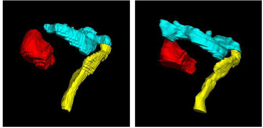
3-D surface renderings of the (red) bladder, (yellow) rectum, and (cyan) sigmoid segmentations by (left) the proposed method and (right) expert radiation oncologist’s manual segmentation on MR1.

As the coarse-to-fine strategy is a key property of the proposed method, an ablation study was conducted to investigate the effectiveness of the coarse segmentation network employed in this study. To this end, two different methods including three independent single-label 3-D U-Nets (i.e., each U-Net segments each OAR), and one 3-D U-Net for multi-label segmentation were tested for coarse segmentation, which yielded the average of DSC for all three organs of 0.85±0.04 and 0.84±0.03, respectively. Since there is no statistically significant difference between the average DSC across all organs for these two approaches (p-value= 0.3882), the single multi-label 3-D U-Net was chosen for coarse segmentation that not only improves the parametric efficiency but also saves time for model training.

We also compared the performance of our 3-D Dense U-Net with a standard 3-D U-Net³¹ and with another 3-D Dense U-Net (referred to as 3-D U-Net+DB which is different from the proposed 3-D Dense U-Net). For both compared methods, we first used the same coarse segmentation network to find the ROI of each OAR but used different fine segmentation networks. The 3-D U-Net used in this comparison for fine segmentation had four encoder-decoder layers in which 16 filters of size 3×3×3 were used in the first layer and were doubled in the subsequent layers. For 3-D U-Net+DB, the same 3-D U-Net was used with modification of adding DB after the second convolution at each layer (notice that we replaced the second convolutional layer with DB in each and every stage in the contraction-expansion paths in the proposed 3-D Dense U-Net.). Therefore, the size of the 3-D U-Net+DB is larger than the proposed 3-D Dense U-Net. The same pre-and post-processing of the MR images as used for the proposed 3-D Dense U-Net were performed for the other networks. All the networks were trained for 200 epochs on MR1 training dataset. Validation metrics were monitored using 10% of the training samples for validation, and the best model was saved as well in conjunction with the training. For all networks, the best saved model was compared with the one saved at the end of 200 epochs, and the network with higher performance was selected for the test. Figure 6 shows example axial MR images overlaid with manual and automatic segmentations. In this example case, the proposed network produced segmentations well-matched to the expert’s manual segmentations while the other two networks failed to do so. Table 1 presents a quantitative performance comparison of the three networks, which shows the superior performance of the proposed method in terms of DSC, as compared to the other two networks. More importantly, our proposed method presents a lower standard deviation value for overall organ segmentation compared to the other methods, which further indicates the effectiveness and robustness of our proposed method. The average of DSC across all organs was calculated and a two-sided paired t-test with α = 0.05 was conducted to investigate the significance of the difference between segmentations computed by different methods. The p-values were estimated as 0.0045 and 0.0023 for a paired comparison of the proposed method with 3-D U-Net and 3-D U-Net+DB, respectively.

Fig. 6.

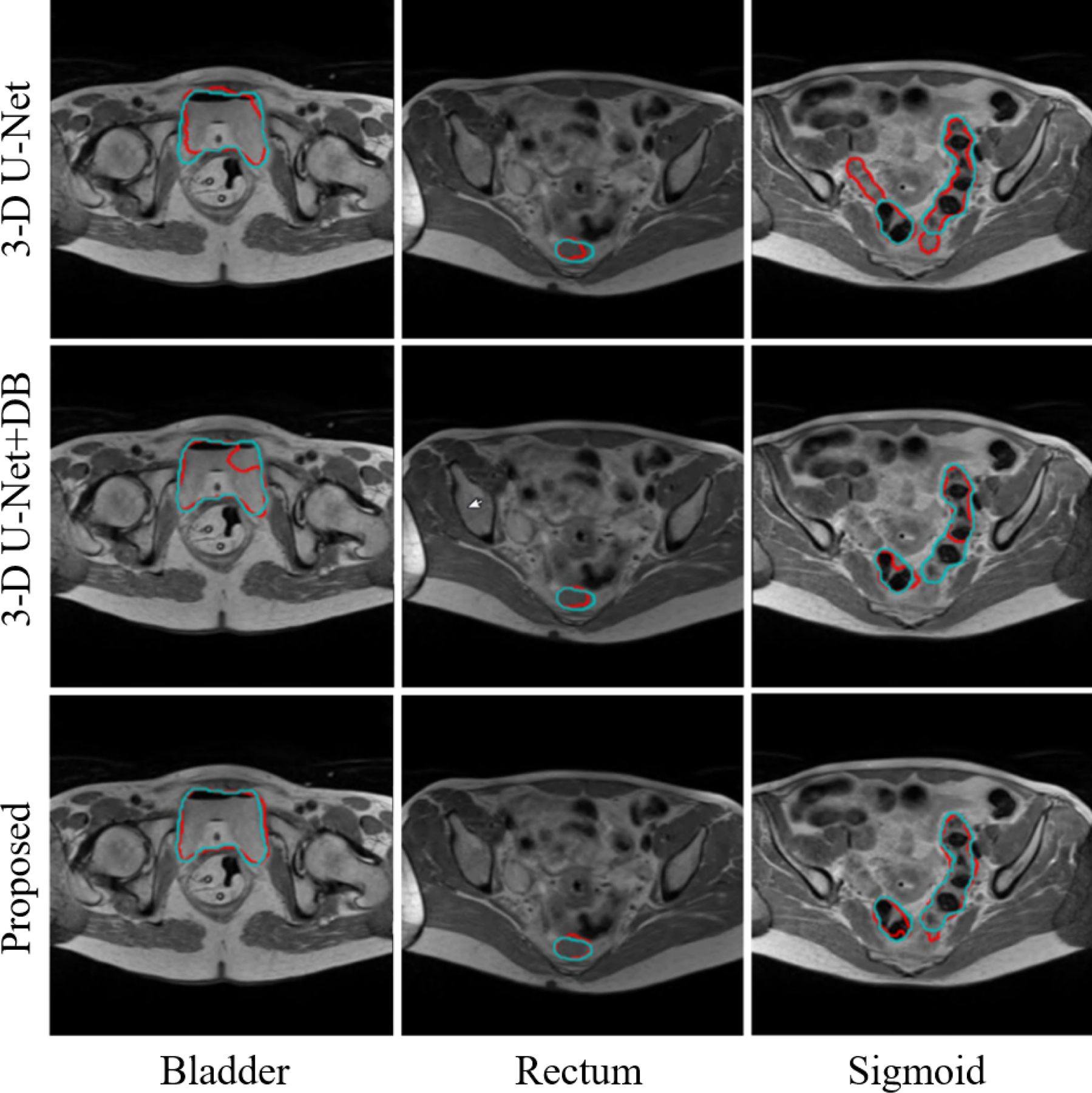
Examples of bladder, rectum, and sigmoid segmentations from MR1 using different methods. (Red) Automatic segmentation. (Cyan) Manual segmentation.

Table 1.

Segmentation performance of three automatic segmentation methods compared to the expert radiation oncologist’s manual segmentations (mean ± SD DSC). Bold indicates the best performance among the three.

	Bladder	Rectum	Sigmoid	Average of all three organs
3-D U-Net	0.85 ± 0.06	0.87 ± 0.03	0.78 ± 0.10	0.83 ± 0.03 (p<0.05)
3-D U-Net+DB	0.86 ± 0.13	0.87 ± 0.04	0.71 ± 0.12	0.81 ± 0.06 (p<0.05)
Proposed	0.93 ± 0.04	0.87 ± 0.03	0.80 ± 0.10	0.87 ± 0.03

Comparison results (Table 1) show that 3-D U-Net+DB yielded a poorer segmentation performance than the standard 3-D U-Net. It might be due to overfitting as adding DB into the 3-D U-Net increases the capacity of the network, but also due to the increased network complexity while the training data remained the same. Considering the limited number of training images in our dataset and limited computing resource, we replaced only the second convolutional layer in the 3-D U-Net instead of adding additional DB in the proposed method. This enables low-level spatial feature preservation, mitigating learning redundant features, and enhancing information flow, while reducing computational complexity. The comparison results presented in Table 1 confirm that this modification improved DSC by 4% and 6% compared to 3-D U-Net and 3-D U-Net+DB, respectively.

3.B. Segmentation on MR2

The proposed networks, fine-tuned on MR2 after being pre-trained on MR1, were tested on 32 MR2 testing samples. Figure 7 illustrates 3-D surface renderings of one sample segmentation. In Fig. 8, example MR2 images from two subjects overlaid with the bladder, rectum, and sigmoid segmentations computed by this method, as compared to the expert’s manual segmentations, are displayed. As shown in both figures and also summarized in Table 2, the automatic segmented OARs were well-matched to the manual segmentations with a DSC (mean±SD) of 0.94±0.05, 0.88±0.04, and 0.80±0.05. Notice that the segmentation performance is equally good on MR2 as on MR1, despite the smaller amount of data in MR2, demonstrating the effectiveness of the proposed active and transfer learning strategy. This may be also due to the improved image contrast in MR2, in which the imaging parameters were tuned to increase the soft tissue image contrast.

Fig. 7.

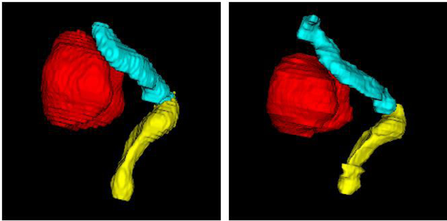
3-D surface renderings of the (red) bladder, (yellow) rectum, and (cyan) sigmoid segmentations by (left) the proposed method and (right) expert radiation oncologist’s manual segmentation on MR2.

Fig. 8.

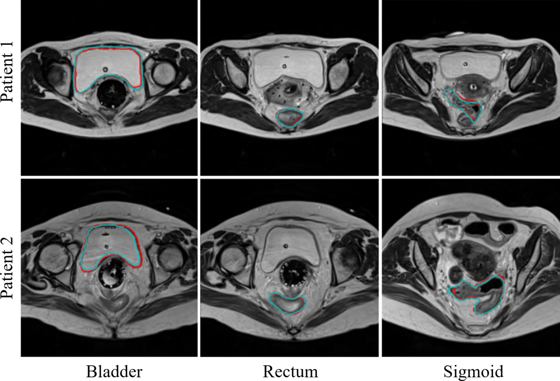
Examples of bladder, rectum, and sigmoid segmentations from MR2 using the proposed method. (Red) Automatic segmentation. (Cyan) Manual segmentation.

Table 2.

Quantitative evaluation of the OAR segmentations on MR2 test data (mean ± SD).

	Bladder	Rectum	Sigmoid	Average of all three organs
DSC	0.94 ± 0.05	0.88 ± 0.04	0.80 ± 0.05	0.87 ± 0.03
AVD (cc)	28.93 ± 35.25	10.66 ± 9.04	12.25 ± 11.25	17.58 ± 13.77
HD95 (mm)	2.89 ± 0.33	2.24 ± 0.40	3.28 ± 1.08	2.80 ± 0.43
Recall (%)	96.19 ± 3.30	86.33 ± 6.46	81.05 ± 8.67	87.86 ± 4.03
Precision (%)	92.53 ± 7.19	90.76 ± 5.01	81.29 ± 8.23	88.19 ± 3.69

Average computation time (including pre-processing, ROI detection by coarse segmentation, fine segmentation, and post-processing) to segment the bladder, rectum, and sigmoid using our model on our MR test images is 11.94±3.11 sec for MR1, and 7.09±3.88 sec for MR2. Note that the computation time for MR1 is longer due to its larger input image size with higher resolution than MR2, which requires longer pre/post-processing time.

To investigate the effectiveness of active and transfer learning, the baseline network was directly applied to MR2 test images without fine tuning. To this end, 50 test images out of 62 were involved in the active learning selection process, among which 30 cases with the lowest DSC scores achieved the baseline network (i.e., considered less predictable by the baseline network thus more valuable for fine-tuning) were used for fine-tuning. The remaining 20 test images (among 50 test images involved in the active learning selection process) were the cases for which the baseline network already achieved relatively higher DSC scores. Consequently, there was only minor improvement of DSC by the fine-tuned network compared to the baseline network. We therefore added 12 additional test cases that were not involved in the active learning selection process, which yielded a total of 32 test cases. The overall DSC for the bladder, rectum, and sigmoid segmentations on these 32 test cases is 0.94±0.05, 0.88±0.04, and 0.80±0.05 (using the fine-tuned network) vs 0.93±0.07, 0.87±0.04, and 0.79±0.08 (using the baseline network). We observed that the overall performance was improved with higher DSC scores and lower standard deviation (note that there are still 20 test cases that are already segmented by the baseline network well). Although the performance is similar for relatively good cases (cases for which the baseline network already works well), the fine-tuned network is particularly effective for cases with poor segmentation accuracy by the baseline network. As an example, the fine-tuned network yielded DSC scores of 0.72 and 0.82 for the bladder and sigmoid for two different cases for each organ while the baseline network yielded 0.63 and 0.58 only (see Fig. 9). These examples demonstrate how much the fine-tuned network improves the segmentation for cases that the baseline network failed to generate acceptable segmentations.

Fig. 9.

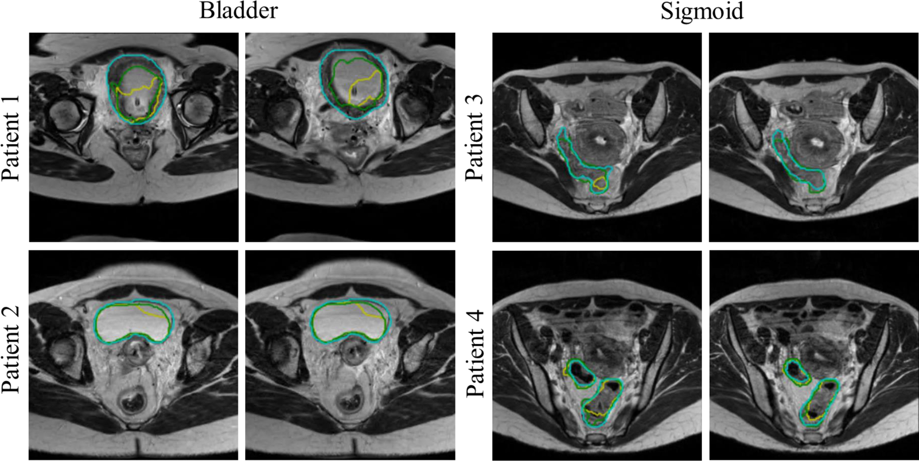
Examples of bladder and sigmoid segmentations from MR2 using the baseline and fine-tuned networks. (Green) Fine-tuned network segmentation. (Yellow) Baseline network segmentation. (Cyan) Manual segmentation.

4. DISCUSSION

In this study, we proposed a fully automated coarse-to-fine CNN approach to segment OARs from MR images. Accurate OAR contouring in female pelvic images is a crucial step for gynecological cancer RT planning, and MRI adds significant value over CT with its superior soft tissue image contrast, thus helping physicians improve contouring accuracy. The presented method is fully automated and is able to rapidly produce high-quality segmentation of OARs from MR images.

In our approach, we augmented 3-D U-Net by replacing the second convolution in every layer with a 3-D DB for fine segmentation of each OAR. The proposed 3-D Dense U-Net showed statistically significant segmentation performance improvement compared to other 3-D-based state-of-the-art CNNs without introducing much additional computational complexity to the model. The proposed 3-D Dense U-Net benefits from a) 3-D operations that allow capturing inter-slice features which are crucial for accurate segmentation of the rectum and sigmoid that show distinct curvatures, b) a U-Net architecture with contraction and expansion paths that enables accurate segmentation via end-to-end training, and c) modified U-Net with embedded 3-D DBs that facilitates better propagation of information through deep networks. Moreover, as our datasets consisted of heterogeneous sets of images, a baseline network was first trained using the dataset with more cases, and then the learned knowledge was transferred to the other dataset, i.e., a new image domain, with fewer cases. We used an active learning strategy in our transfer learning approach to recognize the most valuable data in the target domain for fine-tuning the pre-trained baseline model.

Overall, the experimental results indicate that our method is more accurate in segmenting the bladder and rectum in MR images than for the sigmoid. This is likely due to the complex shape of the sigmoid and its structural variation across different patients. Case by case evaluation revealed that the error for rectum and sigmoid segmentation mostly happens at the conjunction of the rectum and sigmoid. Due to the similar appearance of the rectum and sigmoid, the conjunction region is often segmented as both the rectum (by the rectum segmentation network) and sigmoid (by the sigmoid segmentation network). When merging the independently segmented three organs into a single segmentation volume, we prioritize the segmentation with higher segmentation accuracy. Therefore, for the rectum and sigmoid, the overlapped region is assigned as the rectum since rectum segmentation shows much higher segmentation accuracy than the sigmoid.

Table 3 summarizes the volume distributions of three organs tested in this study. It is evident that the OAR sizes in our dataset vary substantially, which makes the automatic segmentation challenging. Figure 10 illustrates example 3-D renderings of the sigmoid for four different patients, showing how variable the sigmoid shape and size are. Despite such significant variations, our method was able to consistently achieve good segmentation results. To further explore the relationship between the OAR size and segmentation accuracy, the Pearson correlation coefficient between the organ volume and DSC was computed. This metric is reported as 0.3552 (bladder), 0.2010 (rectum), and 0.1694 (sigmoid) on combined MR1 and MR2 datasets, showing small-moderate correlations. For example, the correlation between the bladder volume and DSC is shown in Fig. 11.

Table 3.

OAR volume information in the dataset used to train and test the proposed method.

Dataset	Volume	Bladder (cc)	Rectum (cc)	Sigmoid (cc)
MR1	Minimum	13.58	13.86	3.11
	Maximum	761.53	156.64	137.32
	Mean	183.84	49.72	43.13
	SD	145.22	22.12	28.46
	Median	139.22	44.40	38.14
MR2	Minimum	20.22	19.43	8.42
	Maximum	666.88	100.07	143.80
	Mean	210.21	46.19	43.87
	SD	120.15	16.39	29.30
	Median	191.57	46.34	35.12

Fig. 10.

3-D surface renderings of the sigmoid for four patients selected randomly from our dataset.

Fig. 11.

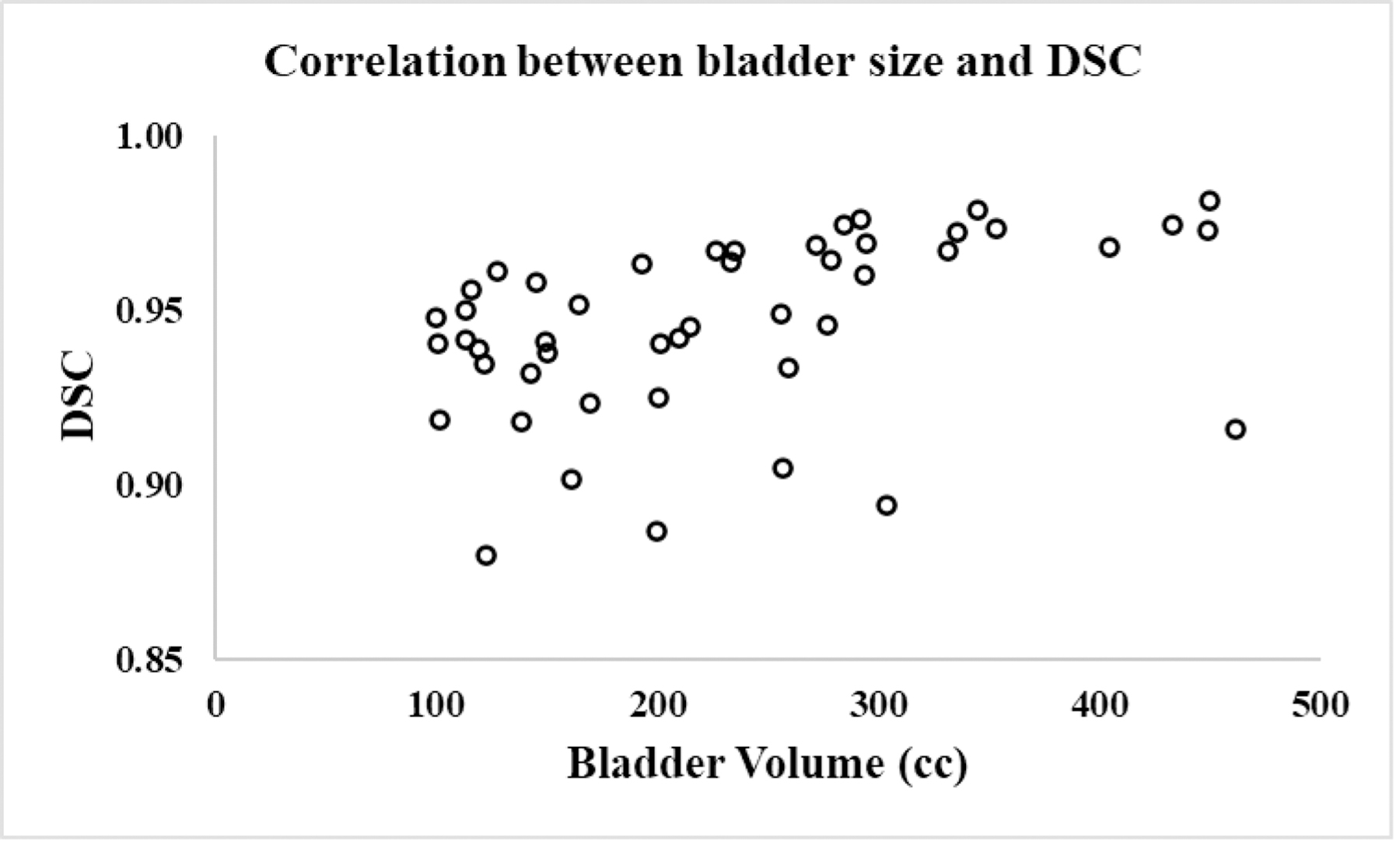
Scatter plot showing correlation between the bladder volume and DSC.

Prior methods for automatic pelvic organ segmentation from MR images have been mostly focusing on male pelvic images, i.e., prostate cases, and DL-based methods have been widely employed⁹. Few methods were previously proposed and tested for female pelvic organ segmentations, among which only one study used MRI data³² while the rest used CT^4–8. Feng et al.³² developed a method for the uterus, rectum, bladder, and levator ani muscle segmentation in female pelvic MRI by combining a CNN and a level-set method where a multi-resolution features pyramid module is introduced into an encoder-decoder model. Their method yielded a DSC of 0.85±0.10 (bladder) and 0.64±0.02 (rectum). Rhee et al.⁴ employed a CNN-based model to first identify CT slices containing the organs of interest, followed by each organ segmentation using a U-Net that achieved a DSC of 0.89±0.09 (bladder) and 0.81±0.09 (rectum). Liu et al.⁵ designed a multi-class segmentation model based on U-Net to segment OAR from CT images and reported a DSC of 0.92±0.05 (bladder) and 0.79±0.03 (rectum). Although the comparison is indirect due to different datasets and imaging modalities used in these studies, our method shows substantially better bladder and rectum segmentation performance than these state-of-the-art methods.

For sigmoid, Gonzalez et al.³³ recently developed an iterative 2.5-D DL-based approach to perform slice-by-slice segmentation in CT images. Even though this method yielded higher DSC (0.82±0.01), it is semi-automatic. Furthermore, unlike a typical CT that has large enough superior-inferior (SI) coverage, our MR images had a much smaller SI coverage, often capturing only a partial sigmoid. Such inconsistent sigmoid images likely resulted in reduced segmentation performance.

As a coarse-to-fine segmentation strategy is used in the presented method where organ-specific ROI is automatically detected by the coarse segmentation, the detected ROI center may not correspond to the center of OAR, i.e., the organ may be slightly shifted from the center of ROI. The ROI size of each organ was determined considering the size of the organ with added margin that is sufficiently large enough not to miss the whole organ. In all of our test cases, we have not observed any case where the whole organ is not fully included within the ROI after the coarse segmentation step unless it is not fully captured in the original MR images (Notice that the bladder and/or sigmoid often is partially captured within the field of view in the original MRI). Even when the target OAR was slightly undersegmented by the coarse segmentation step, the deviation was not significant in all cases, and the resulting ROI images always covered the target OAR. Although our current ROI sizes are sufficiently large to include the target OAR in our data used in this study, there is a possibility that a patient’s organ may be unusually large and extend beyond our ROI sizes. Such a case can be detected from the coarse segmentation, which then can be corrected manually after the fine segmentation (for the portion not included in the ROI volume) or by using multiple ROI volumes and merged segmentations. There is possibility that the target organ may not be exactly positioned at the center of ROI depending on the coarse segmentation quality. However, our fine segmentation network was trained with augmented cases with random translation and rotation, thus offering robust segmentation performance for slightly off-centered ROI volume as presented in the results. Coarse segmentation may produce false positives on the segmentation map. There are cases in which the coarse segmentation network produces more than one segmented region. Case-by-case evaluation of the results showed that those regions appear as small sparse segmented areas in the segmentation map. As OARs are solid tissues, emerged as one integrated large area on MRI, morphological cleaning was applied to the output segmentation map of OARs in order to remove those small false positives. Since there is a possibility of remaining false positives with a size larger than the threshold defined for morphological cleaning, the centroid of each organ was computed using the median value of the segmented region coordinates rather than the mean value, which is less sensitive to outliers.

To assess the effect of ROI selection on the final segmentation accuracy, we used the radiation oncologists’ manual segmentation to determine the ROI (instead of coarse segmentation). When using the ROIs based on manual segmentations, DSCs for the bladder, rectum, and sigmoid were 0.93±0.03, 0.87±0.03, 0.84±0.06 (p-value=0.16 for all three combined), respectively, for MR1, and correspondingly 0.94±0.04, 0.88±0.03, 0.80±0.05 (p-value=0.25 for all three combined) for MR2. There was no significant segmentation performance difference between using the coarse segmentation and manual segmentation to determine the ROI, proving the robustness of the fine segmentation network to ROI selection.

There are methods such as mask R-CNN³⁴, which are known to show excellent performance in the segmentation and detection due to their capability of simultaneously detecting and segmenting the target. In our approach, separate coarse and fine segmentation networks were favored over such simultaneous detection-segmentation approaches due to their limitations. For example, mask R-CNN requires large memory usage with often slow detection speed as each region proposal requires a full pass of convolutional networks³⁴. Separate coarse segmentation step, on the other hand, offers sufficient organ detection and ROI extraction accuracy, and also gives us more room to design organ-specific fine segmentation networks that may even further improve each organ segmentation performance. Although we used the same fine segmentation network structure for all three organs in this study, we optimized each fine segmentation network for each organ, thus achieving improved segmentation performance. Even though Mask R-CNN simultaneously detects and segments objects on images, in many studies it has been employed for detection but not segmentation because Mask R-CNN did not perform desirably on medical images³⁵. Hussain et al.³⁶ employed Mask R-CNN to localize the kidney on CT images. FCN was then applied for fine segmentation due to the poor segmentation accuracy of Mask R-CNN. Vuola et al.³⁷ demonstrated that the standard 2-D U-Net outperforms Mask R-CNN for nuclei segmentation from a wide variety of different nucleus images including both fluorescence and histology images of varying quality. Wang et al.³⁸ demonstrated that a 2.5-D-based method outperforms Mask R-CNN for liver tumor segmentation significantly. Using coarse segmentation results as an extra channel for fine segmentation and/or jointly training coarse and fine segmentation networks in an end-to-end fashion may improve the segmentation performance. However, these approaches increase the network size, and given limited training samples and computing power, increasing the network complexity will likely lead to decreased overall performance.

The coarse segmentation network, trained with DSC, was able to detect OARs with sufficient accuracy, i.e., not producing inaccurate segmentations leading to missing any OAR during the ROI cropping, in all test cases. However, more sophisticated similarity computation considering the organ size such as normalized DSC may be needed especially when including other organs with much more size variation beyond the three organs tested in this study. Jadon³⁹ listed some other improved loss functions for medical image segmentation where their usage can help in fast and better convergence of a model confronting highly imbalanced data.

Our study has several limitations. All the images used in this study were obtained using the same MRI scanner at a single institution, which may introduce bias into the results. Additionally, each patient image was contoured by a single radiation oncologist, although different radiation oncologists contoured different patients’ images, which led to inconsistent manual segmentations, especially for the rectum and sigmoid. It is of our interest to assess inter-observer contouring variability in female pelvic MR images and its impact on the DL-based automatic segmentation performance.

5. CONCLUSIONS

We proposed a fully automated DL-based method to segment multiple organs from female pelvic MR images. Our model offers fast, accurate, and robust automatic segmentation of multiple organs with variable shapes and sizes. Experimental results confirm its superior performance compared to other state-of-the-art methods. Although tested on female pelvic MR images in this study, the proposed method can be adapted to any image-guided procedures where accurate OAR segmentation is needed, obviating the need for tedious manual contouring.

DATA AVAILABILITY

Author elects to not share data.

REFERENCES

- 1.World Cancer Research Fund International. Cervical cancer statistics 2018. https://www.wcrf.org/dietandcancer/cancer-trends/cervical-cancer-statistics. Accessed July 31, 2020.
- 2.Fitzmaurice C, Abate D, Abbasi N, et al. Global, Regional, and National Cancer Incidence, Mortality, Years of Life Lost, Years Lived with Disability, and Disability-Adjusted Life-Years for 29 Cancer Groups, 1990 to 2017: A Systematic Analysis for the Global Burden of Disease Study. JAMA Oncology 2019; 5(12):1749–1769. [DOI] [PMC free article] [PubMed] [Google Scholar]
- 3.Sunil RA, Devang Bhavsar, Shruthi MN, et al. Combined external beam radiotherapy and vaginal brachytherapy versus vaginal brachytherapy in stage I, intermediate- and high-risk cases of endometrium carcinoma. J Contemp Brachytherapy 2018; 10(2):105–114. [DOI] [PMC free article] [PubMed] [Google Scholar]
- 4.Rhee DJ, Jhingran A, Rigaud B, et al. Automatic contouring system for cervical cancer using convolutional neural networks. Med. Phys 2020; 47(11):5648–5658. [DOI] [PMC free article] [PubMed] [Google Scholar]
- 5.Liu Z, Liua X, Xiao B, et al. Segmentation of organs-at-risk in cervical cancer CT images with a convolutional neural network. Phys. Medica 2020; 69:184–191. [DOI] [PubMed] [Google Scholar]
- 6.Kazemifar S, Balagopal A, Nguyen D, et al. Segmentation of the prostate and organs at risk in male pelvic CT images using deep learning. Biomed Phys Eng Express 2018; 4(5):55003. [Google Scholar]
- 7.Balagopal A, Kazemifar S, Nguyen D, et al. Fully automated organ segmentation in male pelvic CT images. Phys Med Biol 2018; 63(24):245015. [DOI] [PubMed] [Google Scholar]
- 8.Sultana S, Robinson A, Song DY, et al. Automatic multi-organ segmentation in CT images using hierarchical convolutional neural network. Journal of Medical Imaging 2020; 7 (5): 055001. [DOI] [PMC free article] [PubMed] [Google Scholar]
- 9.Litjens G, Toth R, van de Ven W, et al. Evaluation of prostate segmentation algorithms for MRI: The PROMISE12 challenge. Med. Image Anal 2014; 18(2):359–373. [DOI] [PMC free article] [PubMed] [Google Scholar]
- 10.Klein S, van der Heide UA, Lips IM, et al. Automatic segmentation of the prostate in 3D MR images by atlas matching using localized mutual information. Med. Phys 2008; 35(4):1407–1417. [DOI] [PubMed] [Google Scholar]
- 11.Liao S, Gao Y, Shi Y, et al. Automatic prostate MR image segmentation with sparse label propagation and domain-specific manifold regularization. in Proc. Int. Conf. Inf. Process. Med. Imag., 2013; 23:511–23. [DOI] [PMC free article] [PubMed] [Google Scholar]
- 12.Toth R, Bloch BN, Genega EM, et al. Accurate prostate volume estimation using multifeatured active shape models on T2-weighted MRI. Acad. Radiol 2011; 18(6):745–754. [DOI] [PubMed] [Google Scholar]
- 13.Qiu W, Yuan J, Ukwatta E, et al. Dual optimization based prostate zonal segmentation in 3D MR images. Med Image Anal 2014; 18(4):660–673. [DOI] [PubMed] [Google Scholar]
- 14.Nie D, Wang L, Gao Y, et al. STRAINet: Spatially Varying sTochastic Residual AdversarIal Networks for MRI Pelvic Organ Segmentation. IEEE Trans. Neural Networks Learn. Syst 2019; 30(5):1552–1564. [DOI] [PMC free article] [PubMed] [Google Scholar]
- 15.Yu L, Yang X, Chen H, et al. Volumetric convnets with mixed residual connections for automated prostate segmentation from 3D MR images. in Proc. AAAI 2017; pp. 66–72. [Google Scholar]
- 16.Zabihollahy F, Schieda N, Krishna S, et al. Automated segmentation of prostate zonal anatomy on T2-Weighted (T2W) and apparent diffusion coefficient (ADC) map MR images using cascaded U-nets. Med Phys 2019; 46(7):3078–3090. [DOI] [PubMed] [Google Scholar]
- 17.Zabihollahy F, Ukwatta E, Krishna S, et al. Fully Automated Detection of the Prostate Peripheral Zone Tumors on Apparent Diffusion Coefficient Map MR Images Using Ensemble Learning Technique. JMRI 2019; 51(4):1223–1234. [DOI] [PubMed] [Google Scholar]
- 18.Zhu Q, Du B, Turkbey B, et al. Deeply-supervised CNN for prostate segmentation. in Proc. Int. Joint Conf. Neural Netw. (IJCNN). 2017; pp. 178–184. arXiv:1703.07523v3. [Google Scholar]
- 19.Liu Y, Yang G; Afshari Mirak S, et al. Automatic Prostate Zonal Segmentation Using Fully Convolutional Network with Feature Pyramid Attention. IEEE Access 2019; 7: 163626–163632. [Google Scholar]
- 20.Li X, Chen H, Qi X, et al. H-DenseUNet: Hybrid Densely Connected UNet for Liver and Tumor Segmentation from CT Volumes. IEEE Trans. Med. Imaging 2018; arXiv:1709.07330v3. [DOI] [PubMed] [Google Scholar]
- 21.Huang G, Liu Z, van der Maaten L, et al. Densely Connected Convolutional Networks. Computer Vision and Pattern Recognition, CVPR 2017 2017. arXiv:1608.06993v5. [Google Scholar]
- 22.Cao Y, Liu S, Peng Y, et al. DenseUNet: Densely connected UNet for electron microscopy image segmentation. IET Image Process 2020; 14(12): 2682–2689. [Google Scholar]
- 23.Zhou Z, Shin J, Zhang L, et al. Fine-tuning convolutional neural networks for biomedical image analysis: Actively and incrementally. in Proceedings - 30th IEEE Conference on Computer Vision and Pattern Recognition, CVPR2017. 2017; pp. 7340–7349. [DOI] [PMC free article] [PubMed] [Google Scholar]
- 24.Zabihollahy F, Rajchl M, White JA, et al. Fully Automated Segmentation of Left Ventricular Scar from 3D Late Gadolinium Enhancement Magnetic Resonance Imaging Using a Cascaded Multi-Planar U-Net (CMPU-Net). Med. Phys 2020; 47(4):1645–1655. [DOI] [PubMed] [Google Scholar]
- 25.Zabihollahy F, Schieda N, Krishna S, et al. Ensemble U-Net-Based Method for Fully Automated Detection and Segmentation of Renal Masses on Computed Tomography Images. J. Med. Phys 2020; 47(9):4032–4044. [DOI] [PubMed] [Google Scholar]
- 26.Cao Z, Yu B, Lei B, et al. Cascaded SE-ResUnet for segmentation of thoracic organs at risk. Neurocomputing 2021; 453: 357–368. [Google Scholar]
- 27.Siddique N, Sidike P, Elkin C, et al. U-Net and its variants for medical image segmentation: theory and applications 2020. arXiv:2011.01118v1. [Google Scholar]
- 28.Tajbakhsh N, Shin JY, Gurudu SR, et al. Convolutional Neural Networks for Medical Image Analysis: Full Training or Fine Tuning? IEEE Trans. Med. Imaging, 2016; 35(5):1299–1312. [DOI] [PubMed] [Google Scholar]
- 29.Raghu M, Zhang C, Kleinberg J, et al. Transfusion: Understanding transfer learning for medical imaging. in Proceedings IEEE Conference on Computer Vision and Pattern Recognition, CVPR 2019. 2019. arXiv:1902.07208v3. [Google Scholar]
- 30.Zeiler MD. ADADELTA: an adaptive learning rate method. Machine Learning 2012. arXiv:1212.5701v1. [Google Scholar]
- 31.Çiçek Ö, Abdulkadir A, Lienkamp SS, et al. 3D U-net: Learning dense volumetric segmentation from sparse annotation. in Lecture Notes in Computer Science (including subseries Lecture Notes in Artificial Intelligence and Lecture Notes in Bioinformatics). 2016. arXiv:1606.06650v1. [Google Scholar]
- 32.Feng F, Ashton-Miller JA, DeLancey JOL, et al. Convolutional neural network-based pelvic floor structure segmentation using magnetic resonance imaging in pelvic organ prolapse. Med. Phys, 2020; 47(9):4281–4293. [DOI] [PubMed] [Google Scholar]
- 33.Gonzalez Y, Shenab C, Jung H, et al. Semi-automatic sigmoid colon segmentation in CT for radiation therapy treatment planning via an iterative 2.5-D deep learning approach. Med. Image Anal 2021; 68:101896. [DOI] [PMC free article] [PubMed] [Google Scholar]
- 34.Hu Q, Souza LF de F, Holanda GB et al. An effective approach for CT lung segmentation using mask region-based convolutional neural networks. Artificial Intelligence in Medicine, 2020; 103:101792. [DOI] [PubMed] [Google Scholar]
- 35.Shu JH, Nian FD, Yu MH, et al. An Improved Mask R-CNN Model for Multiorgan Segmentation. Math Problems in Eng, 2020; [Google Scholar]
- 36.Hussain MA, and Hamarneh G, Cascaded Regression Neural Nets for Kidney Localization and Segmentation-free Volume Estimation. IEEE TMI, 2021; 40(6): 1555–1567. [DOI] [PubMed] [Google Scholar]
- 37.Vuola AO, Akram SU, and Kannala J, mask-rcnn and u-net ensembled for nuclei segmentation. ISBI, 2019; arXiv:1901.10170v1. [Google Scholar]
- 38.Wang X, Han S, Chen Y, et al. Volumetric Attention for 3D Medical Image Segmentation and Detection. MICCAI 2019. [Google Scholar]
- 39.Jordan S, A survey of loss functions for semantic segmentation 2020; arXiv:2006.14822v4. [Google Scholar]
Associated Data
This section collects any data citations, data availability statements, or supplementary materials included in this article.
Data Availability Statement