Full-view in vivo skin and blood vessels profile segmentation in photoacoustic imaging based on deep learning

Abstract

Photoacoustic (PA) microscopy allows imaging of the soft biological tissue based on optical absorption contrast and spatial ultrasound resolution. One of the major applications of PA imaging is its characterization of microvasculature. However, the strong PA signal from skin layer overshadowed the subcutaneous blood vessels leading to indirectly reconstruct the PA images in human study. Addressing the present situation, we examined a deep learning (DL) automatic algorithm to achieve high-resolution and high-contrast segmentation for widening PA imaging applications. In this research, we propose a DL model based on modified U-Net for extracting the relationship features between amplitudes of the generated PA signal from skin and underlying vessels. This study illustrates the broader potential of hybrid complex network as an automatic segmentation tool for the in vivo PA imaging. With DL-infused solution, our result outperforms the previous studies with achieved real-time semantic segmentation on large-size high-resolution PA images.

1. Introduction

Photoacoustic microscopy (PAM) is described as a kind of hybrid biomedical imaging modality based on combining ultrasonic emission and optical excitation [1], [2]. In PAM, a short-pulse laser is absorbed by biological tissues, inducing photothermal effect which includes thermal-elastic expansion that generates an ultrasonic pressure. The rising pressure emits the photoacoustic (PA) waves, which are acquired by an ultrasonic transducer to transform PA images deposition inside the tissue for preclinical and clinical research. PAM provides a three-dimensional (3D) high-resolution images in combination with point-by-point scanning, which utilizes either focused optical beam excitation or focused acoustic beam detection [3]. The present trends are usually research on improving PAM imaging speed while maintaining a highly sensitive detection and high spatial resolution, such as microelectromechanical system (MEMS), galvanometer scanner, polygon scanners, and voice-coil and slider-crank scanning system [3], [4], [5], [6], [7], [8], [9]. Due to the fast imaging with high-quality standards, fast computational technique based on deep learning is essentially important.

PAM has been found to be safe to humans; it has been widely used to image the structure of microvasculature [9], [10], [11]. Furthermore, PAM has great advantages for imaging the functional properties (such as oxygen saturation, hemoglobin concentration, and blood flow), which are crucial for the diagnosis, staging, and study of vascular diseases like diabetes, stroke, cancer, and neural degenerative diseases [12]. However, in human imaging, the generated PA signals on skin (highly absorption of melanin) dominate the inside PA signals leading to unrevealed the internal structure tissue directly. Therefore, blood vessels segmentation and reconstruction in PAM is a vital step in imaging functions and structures of subcutaneous microvasculature. Many efforts have focused on blood vessels segmentation in PAM images, which is a basic method performed by clinical experts who have experience on anatomical tissues. With every B-scan image, skin profile and vessels profile were selected manually [13]. Therefore, this method is not suitable with high-resolution imaging, due to the large number of B-scan images which might exceed over a thousand; most clinical experts identify the manual operation as a time-consuming process to perform. Khodaverdi et al. [14] demonstrated segmentation by approaching adaptive threshold based on statistical characteristics of the background, but the result led to over-segmentation due to the low morphological sensitivity of PA blood vessels signal. In another method, Baik et al. [15] used multilayered based on image depth threshold, by using a local maximum amplitude projection (MAP), instead of the global maximum value, which is commonly used in ultrasonic testing system (also call gate selection) [16]. However, the choice of depth location and threshold is fixed for all the images; signal might be out of range depending on the gate length due to motion artifacts and different tissue types, which could affect the accuracy of the imaging. An early automatically detectable skin profile in volumetric PAM data was developed to find the skin contour on the B-scan images [17], but this technique requires two-round scanning, making it inappropriate for preclinical or clinical application.

Deep learning (DL) approaches, e.g., convolutional neural networks (CNN), have recently exhibited state-of-the-art performance on PA imaging applications. Several review articles as regard to DL applications for PAM imaging have been discussed by Yang et al. and Deng et al., wherein different relevant research articles were explained [18], [19]. Another important review article by Grohl et al. [20] presented the current advancement regarding DL in PA imaging. DL has been determined to be applicable in a variety of aspects for PAM such as image reconstruction [21], [22], [23], [24], [25], image classification [26], quantitative imaging [27], image detection, [28] and, especially, image segmentation [26], [29], [30], [31], [32], [33]. However, those studies almost have been reported about segmentation of the C-scan image (MAP image domain) [26], [29], [31], [32], [33], not widely applied to 3D PA images for separating skin and blood vessels areas. Unlike other works, Chlis et al. [30] used a DL method for processing the cross-sectional B-scan image to avoid the rigorous and time-consuming manual segmentation. However, the requirement input image for this algorithm is fixed, that is, 400 × 400 pixels; it may likely be difficult to fully view small vessel features in the axial and lateral resolution. Thus, an automatic algorithm for segmentation in high-resolution PA images using DL is deemed necessary.

In this research work, we propose a DL method for the segmentation of skin and blood vessels profile PAM images in 3D volumetric data, leveraging the pre-trained 2D model on B-scan dataset. By performing full-form CNN semantic segmentation approaches (U-Net) [34], the technique proposes an automatic skin and vessels segmentation ability for in vivo PA imaging of humans. The key approaches of our research are 3D volumetric segmentation and full-image reconstruction, as it offers a solution in keeping the standards quality high with excellent imaging. However, we could not compare the explicit and quantity metrics because it was not specified in the references [17], [30]. The results are often evaluated in terms of accuracy, Intersection over Union (IoU), sensitivity, and boundary F1 (BF) score and are compared with other popular semantic segmentation models such as SegNet [35], and fully convolutional networks (FCN) [36]. Skin and vessels profiles on each B-scan image were detected automatically in approximately 30 ms, which can be achieved in real-time estimation on high-resolution image data (1000 × 1200 pixels), and motion artifacts problem in in vivo experiments [17] could be resolved. Moreover, the DL model was trained on a large number of B-scan images for in vivo testing results of humans as the ground truth; thus, it was validated in preclinical and biomedical research.

2. Methods

2.1. Data preparation

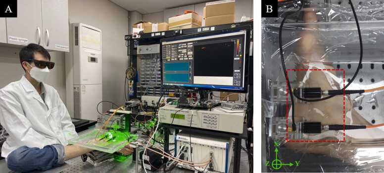
In this study, all of the data were acquired using a dual-fast scanning photoacoustic microscopy system (Ohlabs, Busan, 48513, Republic of Korea) [9]. The three-dimension imaging is acquired by raster scanning of the PA probe over the field of view (FOV) with a step size along both X-axis and Y-axis (Fig. 1(B)). All procedures were performed on a human volunteer following the regulations and guidelines approved by Institutional Review Board of Pukyong National University. The system used 532 nm laser for achieving high absorption coefficients of oxygenated blood with low illumination energy which is under the American National Standards Institute standards safety limit (20 mJ/cm² for 532 nm wavelength) [37]. The acoustic signal was performed by Olympus flat transducer with the central frequency of 50 MHz. Ultrasound signal was acquired for each illumination pulse under a sampling rate of 200 MHz by National Instruments digitizer and was directly fed in to a time series data (A-scan) line. The motion control, laser pulsing and data acquisition are synchronized using LabVIEW software. Fig. 1(A) showed the experimental scheme, images have been obtained from the foot of a volunteer.

Fig. 1.

Experimental setup: (A) Photograph of the experimental set up; (B) Photograph of region of interest (ROI). It represented by red dash box. (For interpretation of the references to color in this figure legend, the reader is referred to the web version of this article.)

2.2. Framework description

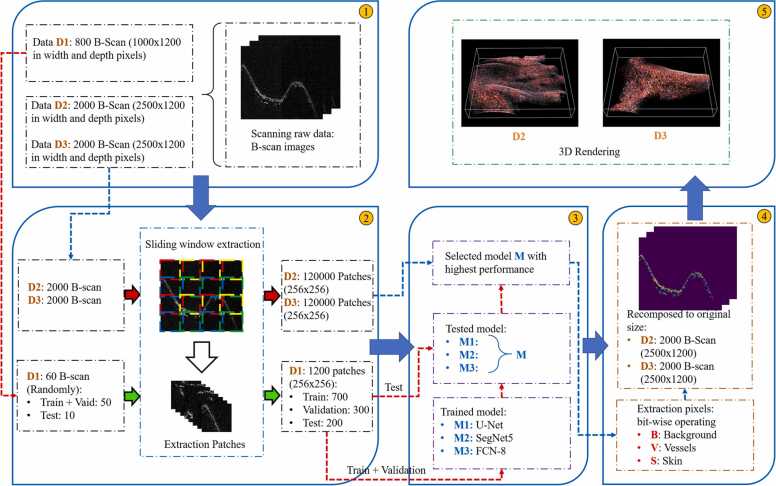
Fig. 2 shows the flowchart for the comprehensive segmentation, which includes preparation input images (1), extraction images (2), DL segmentation network, (3) model comparison, post-processing in skin and blood vessels extraction (4), and (5) 3D rendering. First, human palm and foot were scanned using the PAM system, with rescanning done thrice: D1 and D2 for the palm imaging corresponding to the step size of 0.1 mm and 0.04 mm, and D3 for the foot imaging with the step size of 0.04 mm. All the scanned data was acquired with a 100 × 80 mm² field of view, same step size along both X-axis and Y-axis (Fig. 1(B)), and 1200-sample record along Z-axis at a sample rate of 200 MS/s. By using Hilbert transform in each A-scan, the 2D B-scan images were reconstructed. In total, 800 B-scan images were acquired in D1, while 2000 B-scan images were acquired in D2 and D3. A normalize method was adopted to scale the pixel values to range 0–1, which is preferred for neural network models. For training process, 60 images were chosen randomly from D1 dataset. The original images were extended by sliding window extraction architecture with the stride of S_W = 248 and S_H = 236, which were calculated by sub-multiple finding function. Therefore, the final dataset contains 1200 pairs of the extraction patches (1000 patches for training and validation, 200 patches for testing). In the training process, two classes of object were considered (skin, blood vessels) and the performance of U-Net, SegNet-5 and FCN-8 approach was examined for semantic segmentation of PA images. The accuracy segmented was then compared to other models to evaluate different solutions and find the best results. The highest performance model was utilized to segment the images on D2 and D3 data. For significant standard deviation, the predicted pixel values of each class were arranged in an order from 0 to 1, and the upper 50% (from 0.5 to 1) were set to 1 and lower 50% (less than 0.5) to 0. Bitwise operations were used to extract skin and blood vessels from the images by using a mask which was created by segmentation result via the model. Predicted images were back into original size by inverse sliding window extraction. Finally, 3D geometry and structure of the scanning data were reconstructed by concatenating multiple 2D B-scan images.

Fig. 2.

Deep learning based skin and blood vessels profile segmentation framework for in vivo photoacoustic image.

2.3. CNN networks

2.3.1. U-Net architecture

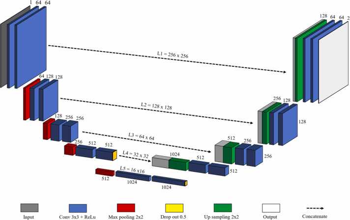
Our method is a direct modification of the completely convolution architecture of U-Net [34], which is well known for its biomedical image segmentation using information from the skip connections. The network consists of a pair of encoder (contraction path) and decoder (expansion path), similar to the original U-Net (Fig. 3). The network takes input size image of 256 × 256 × 1 and then passes through the first convolution block which has two convolution layers; 64 convolution filters, measuring 3 × 3, were then used across the input image to extract 256 × 256 × 64 feature map data. Rectified linear unit (ReLU) activation function was used in converting negative values to 0. Max-pooling process 2 × 2 for downsize of first feature map to 128 × 128 × 64. In the second convolution block, the same convolution layer with keeping the first two dimension of the previous layer and increase the third dimension from 2-times to 128. Max-pooling was used to reduce the dimension to 64 × 64 × 128. The process was repeated twice to reach the bottommost convolution block, which is still built with two convolution layers without max-pooling. Furthermore, dropout was added between two hidden layers having the two largest number of convolutional parameters [38], [39]. Up-sampling path to expand the feature map size from lower resolution to a higher resolution by add some padding on the previous layer followed by a convolution operation. At each up-sampling path, feature map was concatenated with the corresponding feature from the encoder to combine the information from the encoder layer. The process was repeated three more times to back the layer input resolution. The output of the final decoder is fed into a sigmoid activation layer to give the segmentation mask representing the pixel-wise classification.

Fig. 3.

U-Net architecture. The variables L1, L2, L3, L4, L5 refer to the image size (w × h) at the level of different compression depth.

2.3.2. SegNet-5 with Vgg16 backbone

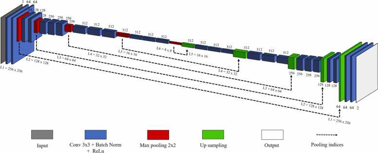
SegNet [35] is described as a semantic segmentation convolutional neural network that consists of an encoder-decoder architecture; it can be classified into SegNet-3 and Segnet-5, depending on the number of convolution blocks inside the model. SegNet-5 is based on Vgg16 [40], which is a popular CNN model in image classification. But the resulting use for segments the image instead of classifying it. In SegNet-5, the encoder path has five convolution blocks (consisting of 13 convolutional layers and 5 max-pooling layers), whereas the decoder path is the opposite of the encoder; however, its max-pooling layer is replaced by pooling indices to match the feature map in up-sampling process. For our modified SegNet-5, we changed the input to grayscale image instead of RGB image. Due to the scanning result, PA image is a grayscale correspond to color images with equal values in all 3-channel. Hence, reducing the input to 1-channel also minimize model parameters [41] without affecting to the input feature map. Moreover, unlike normal classification, medical images classification might belong to more than one class label (mutually inclusive classes) such as many diseases in the same organ [42]. Therefore, we opted for choosing classifications, instead of multiclassification for easily improving our future research with a multi-label segmentation. In the encoders process, the model takes an input image of 256 × 256 × 1 and the passes through five convolution blocks. Each convolution block performs with a dense convolution layer, batch normalization, ReLU activation and 2 × 2 max-pooling layer. Meanwhile, the decoder process is the opposite to that of encoder, wherein it helps in upsizing the feature map at the end of the encoder to the full-size predicted image. Different from the U-Net, during up-sampling process, the max pooling indices at the corresponding encoder layer are recalled to up-sample instead of concatenation to perform convolution. The SegNet-5 architecture is shown in Fig. 4.

Fig. 4.

Architecture of SegNet-5. Where variables L1, L2, L3, L4, L5, L6 refer to the image size (w × h) at the level of different compression depth.

2.3.3. FCN-8 with Vgg16 backbone

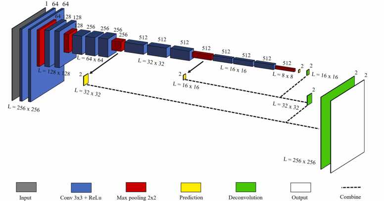
Fully convolutional network (FCN) [36] is one of the first proposed DL method for semantic segmentation. Unlike other approaches where up-sampling process uses mathematical interpolations, FCN uses transposed convolutions layer. Three types of variation are FCN-8, FCN-16 and FCN-32. FCN-32 uses the 32-stride up-sampling at the final prediction layer, whereas FCN-16 and FCN-8 combine with lower layers with more detail in the up-sampling process. In this study, we opted to use FCN-8, which has been identified to have the highest detail feature maps in the up-sampling process. Same with SegNet-5, FCN-8 is also based on Vgg16 network architecture. There are some innovations of using FCN-8 with Vgg16 backbone [43]: Vgg16 use only 3 × 3 convolution filter instead of variable size convolution filter in Alexnet [44] (11 × 11, 5 × 5, 3 × 3), which can reduce parameters and improve the training time; moreover, Vgg16 give the deeper networks and achieve the effect of variable size kernel by implementing the stack of convolutional layers before performing 2 × 2 max pooling layer. FCN-8 takes the input image size of 256 × 256 × 1, in order to obtain the output image of the same size, and transposed convolution was used at the last three down-sampling layers. For up-sampling process, FCN-8 consist 3 deconvolution layers: the first deconvolution layer is 2× up-sample from the last max-pooling layer prediction; the second deconvolution is 2× up-sample from the combination of the first deconvolution layer and second-last max-pooling prediction; the final deconvolution layer performs 8× up-sampling from the fusion of the second deconvolution layer and third-last max-pooling prediction. The number of channels and feature map size corresponding to each step process in FCN-8 are shown in Fig. 5.

Fig. 5.

Architecture of FCN-8. The variable L refers to the image size (w × h) at the level of different compression depth.

2.4. Sliding window architecture

All the models should take 256 × 256 pixel in B-scan images as the input and output images. However, a full B-scan data image might be larger than the required input size; thus, it cannot be directly fed into the model. To overcome this image size limitation concern, we developed sliding window architecture to transform larger images to subset 256 × 256 pixels patches that could be processed using U-Net, SegNet-5, and FCN-8 model and recompose overlap algorithm to transform predicted patches back into the original image size.

Sliding window architecture requires three arguments: first is the image size that the sliding window is going to loop over; second is the window size defined as the width and height of the desired window extract from the full image; and third is the stride size which is indicated as the step size in pixels the sliding window is going to skip.

In order to perform sliding window image selection, the window with size of 256 × 256 like a 2D convolution of a single extractor through the full-sized image and extract the part of the image before were assessed by the trained and predicted model. Stride is the number of pixels shifts over the input matrix, the value of stride height and stride width depends on the full size of the image and sliding window size, were calculated under sub-multiple finding function in Python code. The complete output of the image patches can be calculated using Eq. 1:

$$O=\left(\frac{F_H-K_H}{S_H}+1\right)*\left(\frac{F_W-K_W}{S_W}+1\right)$$ (1)

where F_H and F_W are the height and width of the full-sized image, K_H and K_W are the sliding window height and width (each being 256), and S_H and S_W are stride height and stride width of the sliding window operation. The total patches image O indicates the number of part image after extract through full-sized image given by sliding window technique.

For the inverse sliding window extraction, predicted patches are assumed to overlap and the full-size B-scan image is reconstructed by fulling in the patches from left to right and top to bottom. The overlapping regions were combined by average based on linear blend operator [45]:

$$g\left(x\right)=\frac{f_0\left(x\right)+f_1\left(x\right)}{2}$$ (2)

where g(x) is overlapping regions image, f₀(x) and f₁(x) is two patches which might have some overlapping region.

In this way, we can cover the whole image without resizing the input images. The combination of sliding window architecture and DL model is represented in Fig. 6. The goal of sliding window is to transform high resolution input image into a probability map that corresponds to a ground truth segmentation mask.

Fig. 6.

Block diagram of the Sliding window architecture.

2.5. Training dataset

The D1 dataset contained 800 B-scan images of human palm, all acquired using the PAM system. The data was then randomly split into training set, validation set (50 images), and test set (10 images). Each B-scan image has normalized pixel values, ranging from 0 to 1. For the ground truth image dataset, segmentation mask is a grayscale image (0–255) which was normalized to (0–1), extracted from raw data in PAM system, which were manually segmented by an experienced researcher. For data augmentation, random rotational transform (90, 180 and 270 degrees), random lateral and vertical shift (up to 10% of the image size) [46] were applied to the training set images to tackle model over fitting due to the similarities of images presented by the PA system. The validation dataset used the same data augmentation techniques utilized on the training dataset; none of the augmentation process was used on the testing datasets. The use of sliding window extraction focuses on the segmentation of multiresolution images without resizing method. All the models used the same training parameter in evaluating their performance. The model was trained using a batch size of four images of subset training due to memory constraints. The output layer uses a sigmoid activation to score a prediction of each pixel on patch images. Activation functions are specially used in artificial neural networks to transform an input signal to an output signal [47]. There are many different types of activation functions used in neural networks, depending on the type of neural network and network’s prediction accuracy. Sigmoid function, which can transform the value in range of 0–1, could be defined as $f\left(x\right)=\frac{1}{{1+e}^{-x}}$. The model’s accuracy and model’s loss correspond to the accuracy and loss of the 256 × 256 binary segmentation. The total binary cross entropy loss function L, is used to train the model.

$$L=-\frac{1}{H*W}\sum _{h=1}^H\sum _{w=1}^W\left(y_{\mathit{hw}}*\ln \left(p_{\mathit{hw}}\right)+\left(1-y_{\mathit{hw}}\right)*\ln \left(1-p_{\mathit{hw}}\right)\right)$$ (3)

where H and W correspond to the image height and width in pixels (in this case is 256), $y_{\mathit{hw}}$ and $p_{\mathit{hw}}$ correspond to the ground truth segmentations value and the predicted value for the corresponding pixel at position (h, w), and ln corresponds to the natural logarithm.

TensorFlow [48] is used in implementing the proposed DL approach. The hardware platform we used in this study is a high-performance computer consisting of eight Intel Core i7-6700 (4.00 GHz) and high-speed graphics computing unit NVIDIA GeForce GTX 1060 with 32 GB memory. The networks were set up using Python 3.7 in Keras with a TensorFlow backend. The learning rate of the program is 0.0001 with Adam [49] optimizer algorithm, where the number of iterations is set for 200 epochs. To prevent overfitting, the program is also set for early stopping if the model’s loss on the validation set did not improve for the next 10 patience epochs. ModelCheckPoint callbacks are used to keep the best weight of the model build at each iteration if it achieved minimum validation loss.

2.6. Evaluation methods

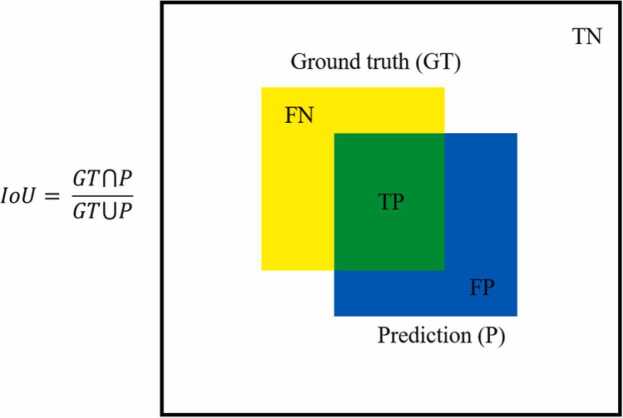
To quantify model performance in segmentation tasks, the performances of U-Net, SegNet-5, and FCN-8 were tested on the testing dataset. Model evaluation is based on four parameters: pixel accuracy, Intersection Over Union (IoU) (Fig. 7), recall (also known as sensitivity), and BF-score [50]. Global accuracy represents the ratio of the highest correctly classified pixels, regardless of all the classes, while accuracy indicates the average percentage of correctly identified pixels for each class.

$$\mathit{ac}\mathit{curacy}=\frac{T_P+T_N}{T_P+T_N+F_P+F_N}$$ (4)

Fig. 7.

Definition of intersection over union (IoU).

IoU is an evaluation metric used to measure the accuracy of predicted bounding box on a ground truth bounding box, whereas mean IoU is defined as the average value over classes. IoU is defined in Eq. 5.

$$\mathit{IoU}=\frac{T_P}{T_P+F_P+F_N}$$ (5)

where T_P, T_N, F_P, and F_N correspond to true positive, true negative, false positive and false negative pixels, respectively. A true positive is a correctly predicted pixels in positive class, a false positive is a falsely predicted pixels in positive class, and the false negative corresponds to a falsely predicted pixels in negative class.

The IoU has been known to be well suited to evaluate the dataset with imbalance class, where more than 90% of the pixels are background. The IoU range from 0–1, where 1 signifying the greatest similarity between ground truth and predicted image.

BF-score measures the proximity and similarity between the predicted boundary and the ground truth boundary, and is given by weighted mean of precision and recall, as defined in Eq. 6.

$$\mathit{BF}=\frac{2*\left(\mathit{precision}*\mathit{recall}\right)}{\mathit{precision}+\mathit{recall}}$$ (6)

where precision is the ratio of true positives and all pixels classified as positives, while ‘recall’ is the ratio of true positives and all positive elements (ground truth).

$$\mathit{precision}=\frac{T_P}{T_P+F_P}$$ (7)

$$\mathit{recall}(\mathit{sensitivity})=\frac{T_P}{T_P+F_N}$$ (8)

2.7. Segmentation in 3D volumetric

The output generated by CNN model is 2-channel tensor binary segmentation mask which is same dimension as the input image. The first channel representing segmentation mask for skin layer and second channel representing for blood vessels layer. In order to divide skin and blood vessels in a 3D volume, mask bitwise operation AND was computed between original 3D data and segmentation mask 3D data. The skin signals were removed by logical bitwise operator AND with blood vessels mask (inversely for blood vessel signal). Finally, the output consists of two 3D segmentation maps for each class (also see in Supplementary Fig. S1).

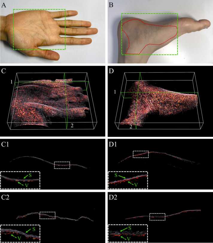
For processing 3D image formats, the input data from segmented image was converted in to NRRD (nearly raw raster data) file, which is a common medical data format for visualization and processing involving three-dimensional raster data. Besides that, the 3D image rendering process is powered by the Visualization Toolkit (VTK) open-source library and CUDA Toolkit GPU-accelerated libraries, which is a powerful tool in visualizing a 3D perspective from multiple 3D images. The imaging results were visualized in graphical user interface designed by Qt creator on C++ platform. To distinguish between the two profiles in a 3D volumetric rendering, scalars to colors converting was applied for each profile with a different colormap (gray-colormap for skin profile and hot-colormap for blood vessels profile). The 3D volumetric segmentation image was show in Fig. 12.

Fig. 12.

Segmentation of skin and blood vessels in 3D volumetric. Photograph of human palm (A), foot (B) with marked region of interest (ROI), represented by dash box; 3D PA images for separating skin and blood vessels areas inside the ROI for (C) human palm, (D) human foot. 3D cross section image at coronal plane (C1) and sagittal plane (C2) as marked in (C). 3D cross section image at coronal plane (D1) and sagittal plane (D2) as marked in (D). White dashed boxes in C1, C2, D1, D2 are the enlarged images of small dashed boxes in each figure. S: Skin and V: Vessel. (For interpretation of the references to color in this figure legend, the reader is referred to the web version of this article.)

3. Results

3.1. Model architecture comparison

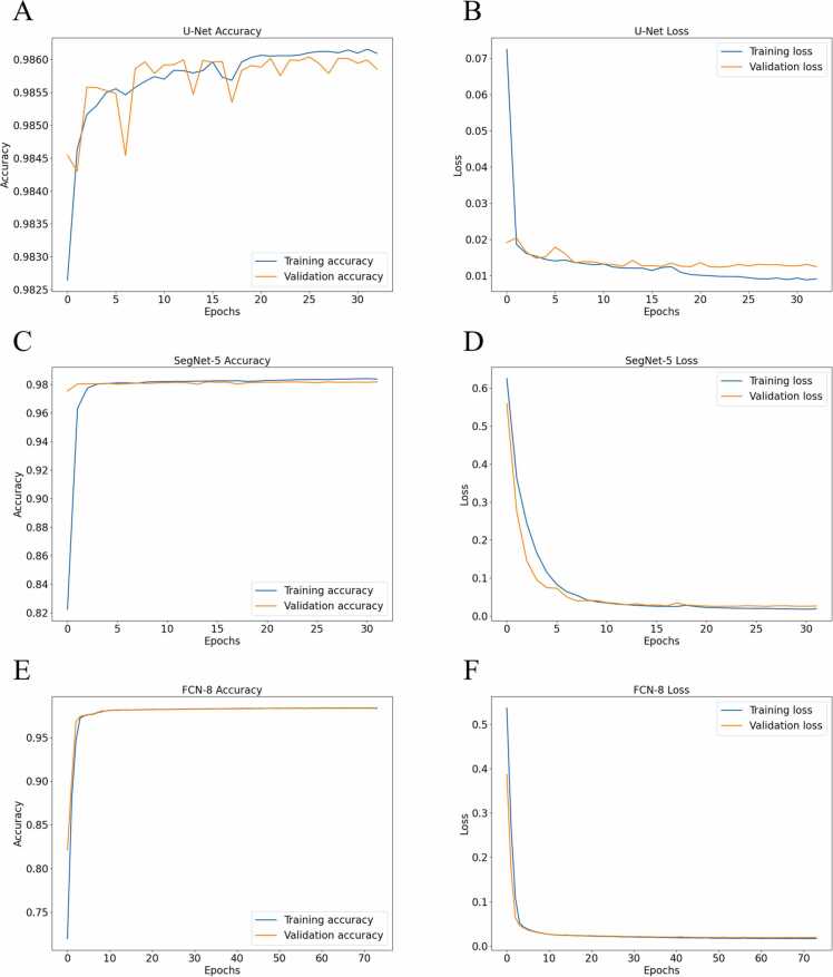
U-Net is trained for 33 epochs due to the early stopping callbacks; the training loss was noted to keep on decreasing, but the validation loss did not improve and started to increase which might be due to overfitting. The SegNet-5 is trained for 32 epochs, where model overfitting is prevented by early stopping callback and dropout layers. FCN-8 is then trained on the same dataset using the same cross entropy loss of function and Adam optimizer with U-Net and SegNet-5. The model is trained for 74 epochs after the early stopping callbacks and stopped it. The training loss kept on decreasing with the number of epochs but the validation did not decrease after the 64th epoch. The accuracy and loss of training and validation are shown in Fig. 8.

Fig. 8.

Model accuracy and loss comparison with respect to the corresponding number of epochs. (A) U-Net accuracy; (B) U-Net loss; (C) SegNet-5 accuracy; (D) SegNet-5 loss; (E) FCN-8 accuracy; (F) FCN-8 loss.

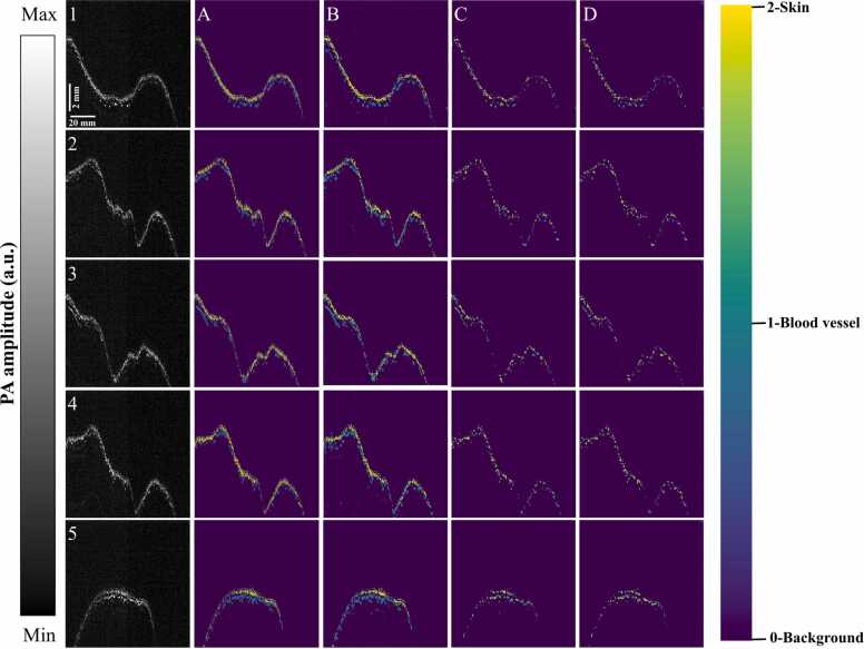
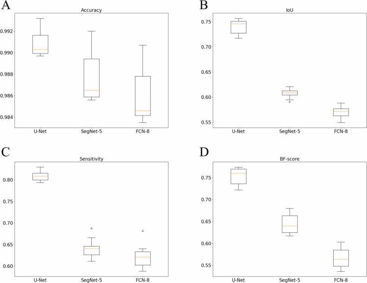
To quantify model performance in segmentation tasks, five evaluation indicators can be observed on testing dataset. The testing dataset includes 10 full-size B-scan images (1000 × 1200 pixels) split randomly from D1 data without any augmentation performance (also see in Fig. 10 and Supplementary Fig. S2). The performance of three models is reported in Table 1 and constructed in Fig. 9. Among the DL methods, FCN-8 exhibited very poor performance, while U-Net was noted to have the best performance. U-Net outperforms FCN-8 by 0.48% in pixel accuracy, 17.12% in IoU, 18.64% in sensitivity, and 18.66% in BF-score. Moreover, the epoch time was reduced by two-times. The SegNet-5 model performance is equivalent to FCN-8, but the number of iterations is not more than twice. SegNet-5 outperforms FCN-8 by 0.16% in pixel accuracy, 3.77% in IoU, 1.86% in sensitivity, and 7.75% in BF-score. To visualize the performance comparison of three model, five examples of segmentation results from the testing dataset are shown in Fig. 10. From column A to D, the image is Ground truth, U-Net, SegNet-5, FCN-8.

Fig. 10.

Visualization of segmentation comparison using different methods on five examples from testing dataset. Column A to D correspond to different method, from left to right: Ground truth, U-Net, SegNet-5, FCN-8; the five examples correspond to five rows from 1 to 5 (please find Supplementary Fig. S2 for examples 6–10).

Table 1.

Statistical metrics (Mean ± standard deviation) comparison of segmentation performance on testing dataset.

	U-Net	SegNet-5	FCN-8
Global accuracy	0.9953 ± 0.0015	0.9938 ± 0.0013	0.9920 ± 0.0019
Accuracy	0.9908 ± 0.0013	0.9876 ± 0.0022	0.9860 ± 0.0025
IoU	0.7406 ± 0.0144	0.6071 ± 0.0091	0.5694 ± 0.0127
Sensitivity	0.8084 ± 0.0109	0.6406 ± 0.0230	0.6220 ± 0.0268
BF-score	0.7529 ± 0.0205	0.6438 ± 0.0231	0.5663 ± 0.0245

Fig. 9.

Boxplots of averaged statistical metrics of U-Net, SegNet-5 and FCN-8 as represented in Table 1. (A) Accuracy; (B) Intersection over Union (IoU); (C) Sensitivity; (D) BF-score.

As shown from visualization results (Figs. 9 and 10), it can be observed that U-Net outperforms SegNet-5 and FCN-8 and demonstrates good reliability and stability. Furthermore, a comparison of training time and memory requirements to train the models is summarized in Table 2.

Table 2.

Comparison of training time and memory requirements for different model.

	U-Net	SegNet-5	FCN-8
Training time (min)	55	59	121
Memory (MB)	3012	2989	2992

3.2. Performance in in vivo PA imaging

U-Net architectures archive the best evaluation in all the performance of CNN models. The U-Net produced better results in segmenting the skin and blood vessels with IoU of 0.74 and BF score of 0.75. These values are reliable for the imbalance class dataset, where background is more than 90% of pixels. Thus, U-Net is the best-suited solution and was chosen to perform segmentation in in vivo PA imaging.

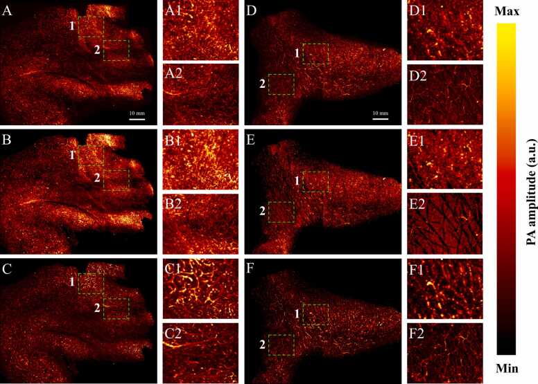
To show the possibility of our model, skin surface and blood vessels profile segmentation were performed on two-sample test: D2 and D3 (PA imaging of a human palm and PA imaging of a human foot). Region of interest inside the red dashed area with an area of 100 × 80 mm² was imaged as shown in Fig. 12(A, B). B-scan images from the scanning data were then fed to the Slide-U-Net (combination of sliding window architecture and U-Net) algorithm, which gives the segmented image. Due to the result of scanning, B-scan image included only two kinds of PA signal: skin and subcutaneous vessels. After feeding B-scan image into the model, images were segmented into two classes binary mask (one-hot encoding) in two-dimensional predicted image. By decode one-hot labels, each segmentation B-scan image is a segmentation map where each pixel contains a class label represented as an integer (as show in Fig. 10): 0 represents background, 1 represents blood vessels profile and 2 represents skin profile. The comparison of in vivo MAP images which were visualized using maximum amplitude projection on each 3D volumetric data (before and after segmentation) along Z-axis is shown in Fig. 11. The detailed PA amplitude image that is overshadowed by mixture signals between the skin surface and underlying vasculature is shown in Fig. 11(A) and Fig. 11(D), but it is clearly visualized in Fig. 11(B, C) and Fig. 11(E, F).

Fig. 11.

Comparison of in vivo MAP image of skin and underlying vasculature in a human palm and foot before and after performing segmentation in Slide-UNET. PA MAP image of human palm (A) and human foot (D) before segmentation. PA image of skin surface structure of human palm (B) and human foot (E) after segmentation. PA image of subcutaneous vasculature structure of human palm (C) and human foot (F) after segmentation. Close-up images of the dashed box regions (1–2) are shown to the right side as (A1), (A2).

The 3D volume was reconstructed by leveraging the union of 2D B-scan images. Each B-scan image was segmented by pre-trained Slide-U-Net algorithm. For illustrative purposes, the image of 3D volumetric segmentation was shown in Fig. 12(C, D) (also see Supplementary Movies 1 and 2). In order to facilitate visualization, results have been projected on the coronal cross-sectional and sagittal cross-sectional planes (Fig. 12(C1, C2, D1, D2)). It is possible to enhance and detect the skin surface and underlying vasculature in a first-person viewpoint.

Supplementary material related to this article can be found online at doi:10.1016/j.pacs.2021.100310.

The following is the Supplementary material related to this article Movie S1, Movie S2..

Further, for comparison of the visibility of the structures in PA image, the peak signal-to-noise ratio (PSNR) between the B-scan image after and before segmentation was approximately 21.3 dB (also see Supplementary Fig. S3). PSNR is defined in the following Eq. 9:

$$\mathit{PSNR}=20*{\mathit{log}}_{10}\left(\frac{{\mathit{MAX}}_I}{\sqrt{\mathit{MSE}}}\right)$$ (9)

where MAX_I is the maximum pixel value of the image (in this case is 255), MSE is mean squared error between the reconstructed PA image before and after segmentation.

4. Discussion

In summary, we designed the DL network architecture for blood vessel segmentation in in vivo PAM imaging. The advantage of this proposed Slide-U-Net approach to learn how to reconstruct and segment images in 3D volumetric data, which might cause mixture signal by using threshold, gate selection and local MAP method. The network architectures require more training time, depending on the number of layers and training parameters, but it gives a segmentation by using the trained model in a few seconds. Our results show a good performance segmentation in two types of PA samples (Fig. 12(A) and (B)) in high-resolution (2500 × 2000 × 1200 in pixel). Slide-U-Net model is not dependent on the size of the input image. Many other studies are reported for image in small resolution (depending on model requirements). Therefore, the segmentation in Slide-U-Net without using the downsize method enables full view with small vessels reconstructing features.

However, there are several restrictions Slide-U-Net algorithm. Firstly, although the sample data (60 full-size B-scan images) in our research is moderately sufficient enough to support the training of the network, the number of data is still limited. Additionally, in data acquisition, our method still has not focused on the impact of ultrasonic frequency, optical wavelength, and scanning method on PAM imaging system. Hence, we plan to conduct more experimental study with more sample data and analyze other effects which have been mentioned above. Secondly, signal processing should be considered for the experimental study. At present, the segmentation model uses the raw data without filtering and denoising signal, which may have some effects on the results. Therefore, we are planning to implement signal processing methods in future study. Thirdly, manual segmentation of the skin and microvasculature requires an experience researcher or clinical expert in photoacoustic imaging. Moving forward, to keep the fully sampled image size, the segmentation procedure for ground truth image dataset may take hours. Finally, our method automatically calculated the stride of sliding window extraction to extract overlap the input image for prediction and reconstruction. If the size of the input image is a prime number, the stride will be one. It can take a longer time for extraction and out of memory when we fed sub-dataset into the model. It will slightly affect the performance of the Slide-U-Net automatic segmentation algorithm in photoacoustic imaging.

5. Conclusions

In conclusion, we were able to successfully apply DL model in reconstructing and segmenting the full-view imaging of PAM. In this study, we have tested and compared on different models and found that U-Net architecture demonstrated the best performance (as described in Table 1). Our Slide-U-Net model outperformed all scanning step-size imaging datasets. The purposed image segmentation techniques are fast and accurate and could help clinical experts in the diagnosis of microvasculature. Furthermore, the results provide a 3D volumetric segmentation image in NRRD file, which is a common type of file format for scientific and medical visualization and could be opened by various medical 3D viewer software.

In the future, the proposed models should be improved in image analysis, along with other modalities of the PAM imaging such as lipids, tumor cells, oxygen saturation, melanoma, and organs. Also, we plan to upgrade the network by incorporating super-resolution training in enhancement of PA images, which can define native image resolution on smaller tissue structures.

Author contribution

C.D.L programmed, designed the DL model, trained, tested, and valuated the data, reconstructed images, as well as prepared the figures for the manuscript. V.T.N, and T.T.H.V acquired the in vivo PAM data, and manually labeled dataset. T.H.V programmed the 3D visualization software. S.M revised the manuscript, interpreted the data. V.T.N, S.P, J.C performed the experiment. J.O and C.S.K conceived and supervised the project. All authors contributed to critical reading of the manuscript.

Declaration of competing interest

The authors declare that they have no known competing financial interests or personal relationships that could have appeared to influence the work reported in this paper.

Biographies

Cao Duong Ly received the B.S. degree in Biomedical Engineering from Ho Chi Minh City University of Technology, Vietnam (2018) and M.S. degree from Pukyong National University, Republic of Korea (2020). He is currently working as a vision engineer and research assistant at Ohlabs Corporation, Busan, Republic of Korea. His research focuses on computer vision for biomedical application and industrial application.

Van Tu Nguyen received the M.Sc. degree in Biomedical Engineering from Pukyong National University, Republic of Korea in 2018. He is currently doing Ph.D. degree in Biomedical Engineering, Pukyong National University. His research focuses on biomedical imaging methods, including photoacoustic imaging and fluorescence imaging.

Tan Hung Vo received the B.S. degree in Ho Chi Minh University of Science, Vietnam (2014). He is currently pursuing the M.S. degree in Biomedical Engineering at Pukyong National University. His research interests Intelligent control based on neural network, Digital image processing.

Sudip Mondal obtained his Ph.D. in 2015 from CSIR-Central Mechanical Engineering Research Institute and National Institute Technology Durgapur, India. He joined as a Post-Doctoral Fellow at Benemérita Universidad Autónoma de Puebla (BUAP) University, Mexico (2015–2017). Currently he works as Research Professor, at the Department of Biomedical Engineering, in Pukyong National University, South Korea. His research interests include nanostructured materials synthesis, bioimaging, and biomedical applications such as cancer therapy and tissue engineering.

Sumin Park received the B.S. degree in Biomedical engineering, Pukyong National University, South Korea (2020). She is currently pursuing her M.S. degree in Industry 4.0 Convergence Bionics Engineering, Pukyong National University, South Korea. Her research interests include fabrication of the transducers, Scanning Acoustic Microscopy, hydroxyapatite and nanoparticles.

Jaeyeop Choi received the B.S. and M.S. degree in Biomedical Engineering from Pukyong National University, Busan, Republic of Korea. He is currently doing Ph.D. degree in Industry 4.0 Convergence Bionics Engineering, Pukyong National University. His current research interests include high frequency ultrasonic transducer and scanning acoustic microscopy.

Thi Thu Ha Vu is pursuing a master’s degree in Industry 4.0 Convergence Bionics Engineering, Pukyong National University, Republic of Korea. Her research focuses on applying Artificial Intelligence, Machine Learning, Deep Learning to Biomedical Image Processing. In addition, she is also working in Image processing in the industrial field.

Chang-Seok Kim received the Ph.D. degree from The Johns Hopkins University, Baltimore, MD, USA, in 2004. He is a Professor with the Department of Optics and Mechatronics Engineering and the Department of Cogno-Mechatronics Engineering, Pusan National University, Busan, South Korea. His current research interests include the development of novel fiber laser systems and application of them into biomedical, telecommunication, and sensor areas.

Junghwan Oh received the B.S. degree in Mechanical engineering from Pukyong National University in 1992, and the M.S. and Ph.D. degrees in Biomedical engineering from The University of Texas at Austin, USA, in 2003 and 2007, respectively. In 2010, he joined the Department of Biomedical Engineering at Pukyong National University, where he is a Full Professor. He also serves as Director of OhLabs Corporation research center. His current research interests include ultrasonic-based diagnostic imaging modalities for biomedical engineering applications, biomedical signal processing and health care systems.

Appendix A. Supplementary material

Supplementary material.

.

Data availability

The python code in Keras with a TensorFlow backend implementation of the Slide-U-Net and all of the training datasets used for this study were acquired by our laboratory are available on Github: https://github.com/lycaoduong/ohlabs_pam_segmentation_unet.

References

- 1.Wang L.V. Multiscale photoacoustic microscopy and computed tomography. Nat. Photonics. 2009;3:503–509. doi: 10.1038/nphoton.2009.157. [DOI] [PMC free article] [PubMed] [Google Scholar]
- 2.Wang L.V., Hu S. Photoacoustic tomography: in vivo imaging from organelles to organs. Science. 2012;335:1458–1462. doi: 10.1126/science.1216210. [DOI] [PMC free article] [PubMed] [Google Scholar]
- 3.Jeon S., Kim J., Lee D., Baik J.W., Kim C. Review on practical photoacoustic microscopy. Photoacoustics. 2019;15 doi: 10.1016/j.pacs.2019.100141. [DOI] [PMC free article] [PubMed] [Google Scholar]
- 4.Yao J., Wang L.V. Photoacoustic microscopy. Laser Photon Rev. 2013;7:758–778. doi: 10.1002/lpor.201200060. [DOI] [PMC free article] [PubMed] [Google Scholar]
- 5.Kim J.Y., Lee C., Park K., Lim G., Kim C. Fast optical-resolution photoacoustic microscopy using a 2-axis water-proofing MEMS scanner. Sci. Rep. 2015;5:7932. doi: 10.1038/srep07932. [DOI] [PMC free article] [PubMed] [Google Scholar]
- 6.Kim J.Y., Lee C., Park K., Han S., Kim C. High-speed and high-SNR photoacoustic microscopy based on a galvanometer mirror in non-conducting liquid. Sci. Rep. 2016;6:34803. doi: 10.1038/srep34803. [DOI] [PMC free article] [PubMed] [Google Scholar]
- 7.Chen J., Zhang Y., He L., Liang Y., Wang L. Wide-field polygon-scanning photoacoustic microscopy of oxygen saturation at 1-MHz A-line rate. Photoacoustics. 2020;20 doi: 10.1016/j.pacs.2020.100195. [DOI] [PMC free article] [PubMed] [Google Scholar]
- 8.Wang L., Maslov K., Yao J., Rao B., Wang L.V. Fast voice-coil scanning optical-resolution photoacoustic microscopy. Opt. Lett. 2011;36:139–141. doi: 10.1364/OL.36.000139. [DOI] [PMC free article] [PubMed] [Google Scholar]
- 9.Nguyen V.T., Truong N.T.P., Pham V.H., Choi J., Park S., Ly C.D., Cho S.-W., Mondal S., Lim H.G., Kim C.-S., Oh J. Ultra-widefield photoacoustic microscopy with a dual-channel slider-crank laser-scanning apparatus for in vivo biomedical study. Photoacoustics. 2021;23 doi: 10.1016/j.pacs.2021.100274. [DOI] [PMC free article] [PubMed] [Google Scholar]
- 10.Mai T.T., Yoo S.W., Park S., Kim J.Y., Choi K.H., Kim C., Kwon S.Y., Min J.J., Lee C. In vivo quantitative vasculature segmentation and assessment for photodynamic therapy process monitoring using photoacoustic microscopy. Sensors. 2021;21:1776. doi: 10.3390/s21051776. [DOI] [PMC free article] [PubMed] [Google Scholar]
- 11.Maneas E., Aughwane R., Huynh N., Xia W., Ansari R., Kuniyil Ajith Singh M., Hutchinson J.C., Sebire N.J., Arthurs O.J., Deprest J. Photoacoustic imaging of the human placental vasculature. J. Biophotonics. 2020 doi: 10.1002/jbio.201900167. [DOI] [PMC free article] [PubMed] [Google Scholar]
- 12.Liu C., Liang Y., Wang L. Single-shot photoacoustic microscopy of hemoglobin concentration, oxygen saturation, and blood flow in sub-microseconds. Photoacoustics. 2020;17 doi: 10.1016/j.pacs.2019.100156. [DOI] [PMC free article] [PubMed] [Google Scholar]
- 13.Maslov K., Stoica G., Wang L.V. In vivo dark-field reflection-mode photoacoustic microscopy. Opt. Lett. 2005;30:625–627. doi: 10.1364/ol.30.000625. [DOI] [PubMed] [Google Scholar]
- 14.Khodaverdi A., Erlöv T., Hult J., Reistad N., Pekar-Lukacs A., Albinsson J., Merdasa A., Sheikh R., Malmsjö M., Cinthio M. Automatic threshold selection algorithm to distinguish a tissue chromophore from the background in photoacoustic imaging. Biomed. Opt. Express. 2021;12:3836–3850. doi: 10.1364/BOE.422170. [DOI] [PMC free article] [PubMed] [Google Scholar]
- 15.Baik J.W., Kim J.Y., Cho S., Choi S., Kim J., Kim C. Super wide-field photoacoustic microscopy of animals and humans in vivo. IEEE Trans. Med. Imaging. 2020;39:975–984. doi: 10.1109/TMI.2019.2938518. [DOI] [PubMed] [Google Scholar]
- 16.B. Yilmaz, A. Ba, E. Jasiuniene, H.K. Bui, G. Berthiau, Comparison of different non-destructive testing techniques for bonding quality evaluation, in: 2019 IEEE 5th International Workshop on Metrology for AeroSpace (MetroAeroSpace), IEEE, 2019, pp. 92–97.
- 17.Zhang H.F., Maslov K.I., Wang L.V. Automatic algorithm for skin profile detection in photoacoustic microscopy. J. Biomed. Opt. 2009;14 doi: 10.1117/1.3122362. [DOI] [PMC free article] [PubMed] [Google Scholar]
- 18.Yang C., Lan H., Gao F., Gao F. Review of deep learning for photoacoustic imaging. Photoacoustics. 2021;21 doi: 10.1016/j.pacs.2020.100215. [DOI] [PMC free article] [PubMed] [Google Scholar]
- 19.Deng H., Qiao H., Dai Q., Ma C. Deep learning in photoacoustic imaging: a review. J. Biomed. Opt. 2021 doi: 10.1117/1.JBO.26.4.040901. [DOI] [PMC free article] [PubMed] [Google Scholar]
- 20.Grohl J., Schellenberg M., Dreher K., Maier-Hein L. Deep learning for biomedical photoacoustic imaging: a review. Photoacoustics. 2021;22 doi: 10.1016/j.pacs.2021.100241. [DOI] [PMC free article] [PubMed] [Google Scholar]
- 21.Lan H., Yang C., Jiang D., Gao F. Reconstruct the photoacoustic image based on deep learning with multi-frequency ring-shape transducer array. Annu. Int. Conf. IEEE Eng. Med. Biol. Soc. 2019;2019:7115–7118. doi: 10.1109/EMBC.2019.8856590. [DOI] [PubMed] [Google Scholar]
- 22.Gutta S., Kadimesetty V.S., Kalva S.K., Pramanik M., Ganapathy S., Yalavarthy P.K. Deep neural network-based bandwidth enhancement of photoacoustic data. J. Biomed. Opt. 2017;22 doi: 10.1117/1.JBO.22.11.116001. [DOI] [PubMed] [Google Scholar]
- 23.Li H., Schwab J., Antholzer S., Haltmeier M. NETT: solving inverse problems with deep neural networks. Inverse Probl. 2020;36 [Google Scholar]
- 24.DiSpirito A., Li D., Vu T., Chen M., Zhang D., Luo J., Horstmeyer R., Yao J. Reconstructing undersampled photoacoustic microscopy images using deep learning. IEEE Trans. Med. Imaging. 2021;40:562–570. doi: 10.1109/TMI.2020.3031541. [DOI] [PMC free article] [PubMed] [Google Scholar]
- 25.Hauptmann A., Lucka F., Betcke M., Huynh N., Adler J., Cox B., Beard P., Ourselin S., Arridge S. Model-based learning for accelerated, limited-view 3-D photoacoustic tomography. IEEE Trans. Med. Imaging. 2018;37:1382–1393. doi: 10.1109/TMI.2018.2820382. [DOI] [PMC free article] [PubMed] [Google Scholar]
- 26.Zhang J., Chen B., Zhou M., Lan H., Gao F. Photoacoustic image classification and segmentation of breast cancer: a feasibility study. IEEE Access. 2019;7:5457–5466. [Google Scholar]
- 27.Cai C., Deng K., Ma C., Luo J. End-to-end deep neural network for optical inversion in quantitative photoacoustic imaging. Opt. Lett. 2018;43:2752–2755. doi: 10.1364/OL.43.002752. [DOI] [PubMed] [Google Scholar]
- 28.Jnawali K., Chinni B., Dogra V., Rao N. Transfer learning for automatic cancer tissue detection using multispectral photoacoustic imaging, Medical Imaging 2019: Computer-Aided Diagnosis. Int. Soc. Opt. Photonics. 2019 doi: 10.1007/s11548-019-02101-1. [DOI] [PubMed] [Google Scholar]
- 29.Boink Y.E., Manohar S., Brune C., Partially-Learned A. Algorithm for joint photo-acoustic reconstruction and segmentation. IEEE Trans. Med. Imaging. 2020;39:129–139. doi: 10.1109/TMI.2019.2922026. [DOI] [PubMed] [Google Scholar]
- 30.Chlis N.K., Karlas A., Fasoula N.A., Kallmayer M., Eckstein H.H., Theis F.J., Ntziachristos V., Marr C. A sparse deep learning approach for automatic segmentation of human vasculature in multispectral optoacoustic tomography. Photoacoustics. 2020;20 doi: 10.1016/j.pacs.2020.100203. [DOI] [PMC free article] [PubMed] [Google Scholar]
- 31.Lafci B., Mercep E., Morscher S., Dean-Ben X.L., Razansky D. Deep learning for automatic segmentation of hybrid optoacoustic ultrasound (OPUS) images. IEEE Trans. Ultrason. Ferroelectr. Freq. Control. 2021;68:688–696. doi: 10.1109/TUFFC.2020.3022324. [DOI] [PubMed] [Google Scholar]
- 32.Ma Y., Yang C., Zhang J., Wang Y., Gao F., Gao F. Human breast numerical model generation based on deep learning for photoacoustic imaging. Annu. Int. Conf. IEEE Eng. Med. Biol. Soc. 2020;2020:1919–1922. doi: 10.1109/EMBC44109.2020.9176298. [DOI] [PubMed] [Google Scholar]
- 33.Lafci B., Merćep E., Morscher S., Deán-Ben X.L., Razansky D. Efficient segmentation of multi-modal optoacoustic and ultrasound images using convolutional neural networks, Photons Plus Ultrasound: Imaging and Sensing 2020. Int. Soc. Opt. Photonics. 2020 [Google Scholar]
- 34.O. Ronneberger, P. Fischer, T. Brox, U-net: convolutional networks for biomedical image segmentation, in: International Conference on Medical Image Computing and Computer-assisted Intervention, Springer, 2015, pp. 234–241.
- 35.Badrinarayanan V., Kendall A., Cipolla R. Segnet: a deep convolutional encoder-decoder architecture for image segmentation. IEEE Trans. Pattern Anal. Mach. Intell. 2017;39:2481–2495. doi: 10.1109/TPAMI.2016.2644615. [DOI] [PubMed] [Google Scholar]
- 36.J. Long, E. Shelhamer, T. Darrell, Fully convolutional networks for semantic segmentation, in: Proceedings of the IEEE Conference on Computer Vision and Pattern Recognition, 2015, pp. 3431–3440. [DOI] [PubMed]
- 37.Zabinski J., American National Standards Institute (ANSI) 2017. Encyclopedia of Computer Science and Technology; pp. 130–132. [Google Scholar]
- 38.G. Chen, P. Chen, Y. Shi, C.-Y. Hsieh, B. Liao, S. Zhang, Rethinking the usage of batch normalization and dropout in the training of deep neural networks, 2019, p. arXiv:1905.05928.
- 39.Lee S., Lee C. Revisiting spatial dropout for regularizing convolutional neural networks. Multimed. Tools Appl. 2020;79:34195–34207. [Google Scholar]
- 40.K. Simonyan, A. Zisserman, Very deep convolutional networks for large-scale image recognition, 2014, p. arXiv:1409.1556.
- 41.Z. Zheng, Z. Li, A. Nagar, W. Kang, Compact deep convolutional neural networks for image classification, in: Proc. ICMEW, 2015, pp. 1–6.
- 42.Maksoud E.A.A., Barakat S., Elmogy M. Machine Learning in Bio-Signal Analysis and Diagnostic Imaging. Elsevier; 2019. Medical images analysis based on multilabel classification; pp. 209–245. [Google Scholar]
- 43.W. Yu, K. Yang, Y. Bai, T. Xiao, H. Yao, Y. Rui, Visualizing and comparing AlexNet and VGG using deconvolutional layers, in: Proceedings of the 33 rd International Conference on Machine Learning, 2016.
- 44.Krizhevsky A., Sutskever I., Hinton G.E. Imagenet classification with deep convolutional neural networks. Adv. Neural Inf. Process. Syst. 2012:1097–1105. [Google Scholar]
- 45.Szeliski R. Springer Science & Business Media; 2010. Computer Vision: Algorithms and Applications. [Google Scholar]
- 46.Shorten C., Khoshgoftaar T.M. A survey on Image Data Augmentation for Deep Learning. J. Big Data. 2019;6:1–48. doi: 10.1186/s40537-021-00492-0. [DOI] [PMC free article] [PubMed] [Google Scholar]
- 47.Sharma S., Sharma S. Activation functions in neural networks. Towards Data Sci. 2017:310–316. [Google Scholar]
- 48.M. Abadi, A. Agarwal, P. Barham, E. Brevdo, Z. Chen, C. Citro, G.S. Corrado, A. Davis, J. Dean, M. Devin, S. Ghemawat, I. Goodfellow, A. Harp, G. Irving, M. Isard, Y. Jia, R. Jozefowicz, L. Kaiser, M. Kudlur, J. Levenberg, D. Mane, R. Monga, S. Moore, D. Murray, C. Olah, M. Schuster, J. Shlens, B. Steiner, I. Sutskever, K. Talwar, P. Tucker, V. Vanhoucke, V. Vasudevan, F. Viegas, O. Vinyals, P. Warden, M. Wattenberg, M. Wicke, Y. Yu, X. Zheng, TensorFlow: large-scale machine learning on heterogeneous distributed systems, 2016, p. arXiv:1603.04467.
- 49.D.P. Kingma, J. Ba, Adam: a method for stochastic optimization, 2014, p. arXiv:1412.6980.
- 50.Costa M.G.F., Campos J.P.M., de Aquino E.A.G., de Albuquerque Pereira W.C., Costa Filho C.F.F. Evaluating the performance of convolutional neural networks with direct acyclic graph architectures in automatic segmentation of breast lesion in US images. BMC Med. Imaging. 2019;19:85. doi: 10.1186/s12880-019-0389-2. [DOI] [PMC free article] [PubMed] [Google Scholar]
Associated Data
This section collects any data citations, data availability statements, or supplementary materials included in this article.
Supplementary Materials