

Summary
The importance of disordered protein states in biology is gaining recognition, and can be attributed in part to the participation of unfolded and partially folded states of globular proteins in normal and abnormal biological functions, such as protein translation, protein translocation, protein degradation, protein assembly, and protein aggregation (1–5). There is also a growing awareness that a significant fraction of gene products from various genomes, including the human genome, fall into a category that includes low complexity, low globularity, or intrinsically unstructured proteins (6–9). Unlike native states of globular proteins, disordered protein states, by definition, do not adopt a fixed structure that can be determined using classical high-resolution methods. Nevertheless, there has long been evidence that many disordered states contain detectable and significant residual or nascent structure (10–16). This structure has been found to be important for nucleating local structure, as well as mediating long range contacts upon either intramolecular folding to the native state (17–21) or intermolecular folding with specific binding partners (22–24), and is also predicted to influence intermolecular folding into structured aggregates (25,26). The primary tool for the characterization of such structure is high-resolution solution state nuclear magnetic resonance (NMR) spectroscopy. Advances in NMR instrumentation and methods have greatly facilitated this task and in principle can now be accomplished by those without extensive prior experience in NMR spectroscopy. This chapter describes how this can be accomplished.
Keywords: Protein folding, residual structure, nascent structure, intrinsically unstructured, natively unfolded, unfolded state, denatured state, molten globule, folding intermediates, NMR, secondary shifts, random coil
1. Introduction
Detailed structural information for the end point of typical protein folding reactions has been available for many decades. Only recently, however, has it become practical to address the structural properties of the ensemble of unfolded states from which folding initiates. Optical methods, such as circular dichroism, fluorescence, and Fourier-transform infrared spectroscopies of unfolded proteins frequently contain evidence for a small, but detectable amount of structure (10), but further characterization of such structure was not often pursued. More recently, this has begun to change.
With the advent of multidimensional solution nuclear magnetic resonance (NMR) spectroscopy it became possible to resolve signals from individual sites in proteins, even in their denatured state (12), and, therefore, to learn about the local environment and structure of these sites. There are two primary requirements for achieving this goal. First, the individual NMR resonances have to be mapped to the corresponding nuclei in the protein from which they originate. This is referred to as the resonance assignment process, and remained the primary hurdle for NMR studies of disordered proteins for some time. Recent advances in NMR methods combined with increased access to high-field and ultra-high-field NMR spectrometers, however, have provided the tools needed to make this a routine task, at least for backbone resonances, and the process will be described in detail in Subheading 4. Once backbone resonance assignments are available, measurable parameters that inform regarding local environment and structure are required. Many such parameters are useful in the high resolution structural characterization of well-folded proteins (27), including chemical shifts, coupling constants, nuclear Overhauser effects (NOEs), relaxation rate constants (28–31), and more recently residual dipolar couplings (32,33). These same parameters can also be used to analyze the structural properties of disordered proteins, but the weak signatures of elements of residual structure require somewhat different considerations.
2. Production of Isotopically Labeled Protein
Like classical NMR structure determination, analyzing residual structure in proteins by NMR is greatly facilitated by the use of isotopically labeled protein, in which 14N and 12C are replaced with 15N and 13C. A requirement for this approach is the ability to produce the protein of interest recombinantly. Although isotopic labeling of proteins produced in yeast and in cell culture is slowly becoming feasible (34,35), these systems are not described here as the great majority of proteins for NMR study are produced in Escherichia coli. Once recombinant protein can be expressed and purified from E. coli, producing isotopically labeled material is usually a simple exercise. To prevent incorporation of unlabeled isotopes into the protein, bacteria are grown on a minimal medium completely lacking in carbon or nitrogen, to which a single source of these elements is then added, typically in the form of ammonium-sulfate or -chloride for nitrogen and glucose for carbon. Usually, minimal media is made using an M9-recipe similar to the one shown in Table 1 (36). Protein yield is typically as much as 50% lower from cultures grown on minimal media, especially when limiting quantities of 13C-labeled glucose are used.
Table 1.
Preparation of Isotopically Labeled Minimal Media
| To make 1 L of 5X M9 salts |
| 34 g of Na2HPO4 (or 36 g of Na2HPO4[H20] or 64 g of Na2HPO4[7H20]) |
| 15 g of KH2PO4 |
| 2.5 g NaCl |
| Bring up volume to 1 L with dH20 and sterilize by autoclaving |
| To make 1 L of 15N- or 15N,13C-labeled minimal media |
| 200 mL of 5X M9 salts |
| 700 mL of sterile dH2O |
| 100 μL of sterile 1 M CaCl2 (add only after other salts are completely dissolved!) |
| 1 mL of sterile 1 M MgSO4 (add only after other salts are completely dissolved!) |
| Dissolve and sterile filter into above: |
| 1.0 g of labeled 15N-labeled ammonium chloride |
| 4.0 g of unlabeled glucose (or 2.0–4.0 g of 13C-labeled glucose) |
| 10 mL of 100X Basal Eagle vitamin mix |
| 30 mL of dH2O |
| Adjust to 1 L with dH 2 0 |
Because disordered proteins are generally quite flexible, the relaxation rates that determine the efficiency of magnetization transfer during the triple-resonance experiments described below are quite favorable. This means that the benefits obtained from triple labeling with 2H, 13C, 15N are not typically needed. If required, highly deuterated samples can be made by using D2O instead of H2O in preparing the M9 media, and uniformly deuterated samples can be produced by using 2H, 13C-labeled glucose as well as D2O. Growing bacterial cultures in D2O-based media leads to a significant (approximately twofold typically) reduction in growth rate, and often leads to a further decrease in protein yield. In order to reduce the amount of D2O and isotopically labeled compounds needed for the production of labeled proteins, it is possible to grow cultures to midlog phase in rich media, spin down the cells, wash them, and then resuspend them in minimal media. The cells should then be given 30–60 min to recover before protein production is induced. Nearly uniform labeling can be achieved in this way with lower costs (37).
3. NMR Sample Preparation
NMR experiments typically require approx 0.5 mL of 13C,15N double-labeled protein at a concentration of approx 0.3 mM. Higher concentrations can provide better signal to noise but should be used with caution, as disordered proteins often aggregate easily. NMR two-dimensional (2D) proton–nitrogen correlation (HSQC) spectra can be used as a diagnostic for aggregation in tandem with other techniques, such as gel filtration or light scattering. The use of NMR tubes with susceptibility-matched plugs (available from Shigemi, Inc. for example) allows sample volumes of 0.25–0.3 mL to be used if sample quantity is limiting. Because the backbone amide protons in disordered proteins are typically not protected from the solvent by either intramolecular hydrogen bonds or burial, samples should be prepared at lower pH if possible to limit the exchange of amide protons with solvent protons (38,39). A pH of 4.0 is ideal for slowing exchange, but is often too low to maintain physiological relevance and can perturb the structure of interest. pH values of up to 7.5 or so can be used successfully by lowering the sample temperature to 10°C or even 5°C. Salt concentrations should be such that ionic strength remains below approx 0.2 mM. If cryogenic probe technology is to be used, sample concentrations can be reduced to approx 0.1 mM in favorable cases, although lower salt concentration and low-conductivity buffers may be necessary to achieve the necessary gain in sensitivity (40).
4. Obtaining NMR Backbone Resonance Assignments for Disordered Proteins
In comparison to well-structured proteins, disordered proteins give rise to crowded, highly degenerate NMR spectra, increasing the challenge of assigning the individual resonances. Nevertheless, certain nuclei in polypeptide backbones retain significant dispersion that can be taken advantage of. In particular, the resonance frequencies or chemical shifts of both backbone 15N nuclei (41) and backbone 13CO nuclei (42,43) are highly sequence dependent, even in the absence of well-ordered structure. In contrast to the 15N and 13CO sites, the chemical shifts of the 13Cα and 13Cβ nuclei in the absence of well-ordered structure are quite degenerate. This, however, can also be made use of, because the combination of these two chemical shifts is highly effective at discriminating between different amino acid side chains (44), and is, therefore, of great use in the assignment process (45). With these considerations in mind, the following set of three-dimensional (3D) triple-resonance experiments can be considered as ideal for obtaining the data necessary for backbone resonance assignments of disordered proteins:
HN(CA)CO (correlates NHi, Ni and COi/i-1).
HNCO (correlates NHi, Ni, and COi-1).
HNCACB (correlates NHi, Ni, and Cα,Cβi/i-1).
CBCA(CO)NH or the equivalent HN(CO)CACB (correlates NHi, Ni, Cα,Cβi-1).
These experiments are available in standard form in the pulse sequence libraries provided by the major manufacturers of NMR spectrometers, and can, therefore, be executed in a straightforward fashion. Although a minimal familiarity with the details of operating a NMR spectrometer is required, sufficient training can be obtained in 1 d, or even a few hours, from a knowledgeable facility manager or user. Processing of the resulting data to produce the 3D spectra is also straightforward, with a variety of software available for the task.
Each of these four experiments results in spectra that contains peaks, or correlations, that are each characterized by three resonance frequencies or chemical shifts: that of a backbone amide proton, of its covalently attached nitrogen, and of the CO, Cα, or Cβ nucleus that belongs to either the same residue (an “i” correlation) or the one immediately preceding it in the protein sequence (an “i–1” correlation). All together, the experiments provide the complete backbone and Cβ chemical shifts for each dipeptide spin system that gives rise to detectable signals. The data can be illustrated schematically for the HN, N, Cα, and CO shifts of a cyclical four-residue peptide as shown in Fig. 1.
Fig. 1.
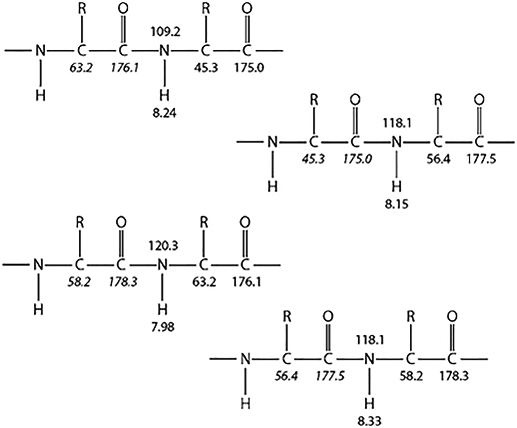
Illustration of dipeptide spin systems constructed using backbone HN, N, Cα, and CO resonances for a hypothetical cyclical four-residue peptide. Inter-residue (i–1) chemical shift correlations are shown in italics.
The process of making sequence-specific resonance assignments involves linking individual dipeptide systems to each other by matching the overlapping chemical shifts, in this case the CO, Cα, and Cβ shifts. Because the Cα and Cβ shifts are highly degenerate, as previously discussed, they are less useful for linking dipeptides than the better dispersed CO shifts. However, the Cα and Cβ shifts can often be used to identify or constrain the specific side chains of each residue in the dipeptide spin system, and this information can be invaluable in placing the dipeptide, and any segments linked to it, into the known sequence of the protein. The process of linking the dipeptide spin systems is illustrated in Fig. 2. Once this basic concept is understood, various techniques can be used to accomplish the task at hand. One approach is to simply select an inter-residue (i–1) peak in one of the spectra and graphically search all other peaks in the appropriate spectrum for the corresponding intraresidue (i) peak. At the other end of the spectrum, one can generate a numerical table of all the correlations, identify the chemical shift of an inter-residue correlation, and search the numerical table for possible matches. Different people typically develop their own preferred approach. Note that although software packages for automated assignments of NMR backbone resonances of proteins (AutoAssign [46], MARS [47], and others) can be highly effective when applied to well-structured proteins, they are typically less successful with spectra from disordered proteins and significant manual effort is usually required.
Fig. 2.
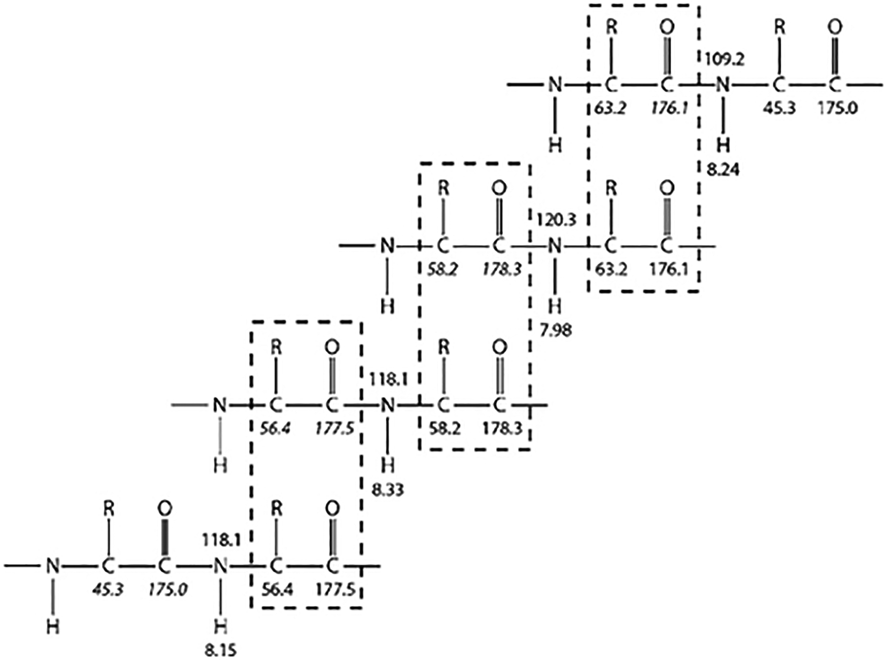
Illustration of resonance assignment process relying on matching resonance frequencies between overlapping regions of different dipeptide spin systems.
5. Identifying Residual Structure
5.1. Chemical Shifts
Once backbone resonance assignments have been obtained, it is possible to begin to learn about the structural preferences of specific residues in the disordered protein of interest. The easiest and perhaps most sensitive parameters to analyze are chemical shifts, many of which are conveniently available immediately from the assignment process. Chemical shifts have proven to be sensitive and accurate predictors of secondary structure (48–54) and this property has been used to develop a robust algorithm to identify secondary structure in well-folded proteins (55,56). Although this algorithm can be applied to several nuclei, its application to Cα shifts will be described here because they have proven to be the most sensitive and accurate predictors of secondary structure, being least affected by other factors (57). The algorithm relies on calculating the differences between each observed chemical shift and the values that would be expected if a given residue were in an idealized random-coil state. The latter values have been estimated either from statistical analyses of chemical shift databases from well-structured proteins (49,54,58), or from direct measurements of chemical shifts from residues in short peptides that contain little or no structural preferences (53,59–62). The differences between the observed and tabulated random-coil shifts are referred to as secondary shifts. Once calculated, secondary shifts are used to predict the presence of helical or strand structure based on their sign, amplitude, and contiguity. For Cα secondary shifts, positive values correlate with helical structure and negative values with strand structure, and the Cα amplitude thresholds used to analyze structure in well-folded proteins are typically 0.5 PPM (63). Uninterrupted stretches of positive or negative secondary shifts above the amplitude threshold indicate helical or strand structure, respectively. The contiguity criterion requires uninterrupted stretches of at least four nonstrand-indicating secondary shifts to establish a helix, and at least three non-helix-indicating values to establish a strand, and in either case, the “density” of helix- or strand-indicating values should exceed 70%.
Although highly successful in identifying and delineating secondary structure elements in well-folded proteins, the previously mentioned algorithm is more difficult to apply to highly disordered proteins because the secondary structure elements are not well formed, being instead transient in nature, and the associated secondary shifts are of much lower amplitude. Nevertheless, Cα secondary shifts in particular still provide highly accurate information if care is taken. When dealing with residual or nascent structure, it is of crucial importance to use the “best” possible random-coil shifts. In contrast to examining well-formed structure, where secondary shifts are relatively large in magnitude (several PPM for Cα), residual structure leads to secondary shifts that are typically quite small (less than 1 PPM and often just a few tenths of a PPM for Cα), so errors in the random-coil shifts can have a profound effect on the results. In general, our experience has indicated that statistically derived random-coil shifts are not as accurate for analyzing poorly structured states as experimentally measured random-coil values. In contrast, the statistical values may be somewhat superior in the prediction of well-formed structure. Of the experimentally determined data sets, the most recent tabulation by Wishart et al. (62), which was obtained at pH 5.0 and 25°C, is in our experience the most accurate for analyzing samples at near physiological pH values, while the data of Schwarzinger et al. (64) is most appropriate for proteins denatured in urea at low pH.
The latter data set was later accompanied by a detailed analysis of sequence-specific corrections to the residue-specific, random-coil shifts (65). Although this analysis demonstrates clearly that these corrections are quite small for the Cα shifts, the corrections do improve the analysis of residual structure (66). However, it should be noted that the corrections may be specific to the conditions used for the measurements, and it is not yet clear if they can be directly applied to residue-specific, random-coil values determined under other conditions. Sequence-specific corrections have also been carefully tabulated by Wang and Jardetzky using a statistical approach (67), but these corrections too, in our experience, cannot be taken out of context and applied to experimentally determined random-coil values. Ultimately, the best possible results can be achieved only by directly measuring random-coil shifts from small peptides, including sequence-specific corrections, under conditions close to those of interest (but note that small peptides can adopt nonrandom structure [66] and such structure must be destabilized). In the absence of such pain-staking measurements, the more appropriate of the Wishart (62) or Schwarzinger (64,65) data sets should be used, but pH differences leading to the titration of side chain groups (Glu, Asp, or His) require corrections for their residues (68). An additional note is that accurate determination of experimental carbon chemical shifts is facilitated by extensive zero filling of data in the carbon dimension. Although the intrinsic resolution of the data is not improved by this procedure, the effective increase in the quality of the interpolation is important for determining the positions of resonances.
Once secondary shifts are calculated using carefully determined Cα chemical shifts and the appropriate random-coil shifts, identifying residual secondary structure follows the same principles used for well-folded proteins. However, the smaller secondary shifts introduce a greater degree of ambiguity into the procedure. In particular, the amplitude threshold must be relaxed. However, the contiguity requirement should typically be increased to compensate. Longer stretches of secondary shifts of the same sign, but where several or even many fall below the amplitude threshold, can be reliable indicators of residual structure. Short (three to four residue) stretches of residual structure are more difficult to diagnose with certainty unless the secondary shifts are all above the threshold value. It should be noted that the availability of any complimentary functional, biochemical, or structural data for the protein of interest can greatly increase the confidence of the chemical shift analysis. This is based on the observation that residual structure is often most evident in regions that are well structured in other contexts (in the native state if one exists, or in a well-defined conformation adopted upon binding to an interaction partner), and that such regions therefore also tend to stand out in biochemical or functional studies employing site-specific or deletion mutagenesis (24,69).
Although Cα secondary shifts are the most accurate indicators of secondary structure, other chemical shifts can also be helpful. Hα secondary shifts in particular are excellent indicators of secondary structure in well-folded proteins because of their great sensitivity to backbone ϕ/ψ angles. However, Hα shifts are also more sensitive than carbon shifts to other factors, such as ring currents, hydrogen bonding, and electrostatic effects (57), which effectively make them “noisier” than Cα shifts when dealing with small amplitude deviations. Nevertheless, Hα shifts are a useful complement to Cα shifts. Similarly, CO and Cβ shifts are also sensitive to secondary structure. While CO shifts show excellent dispersion in well-folded states, much of this dispersion originates from sequence-dependence effects and is, therefore, retained in disordered states. These effects are difficult to correct for, making CO secondary shifts relatively noisy (43). Cβ shifts are somewhat sensitive to strand structure, but are much less sensitive to helical structure (57). They also display considerably less dispersion even in well-folded structures, providing less dynamic range for the detection of residual structure (43). When residual structure is indicated by a consensus of secondary shifts from two or more nuclei, this again greatly increases the reliability of the analysis.
5.2. Nuclear Overhauser Effects
NOEs form the basis of classical structure determination by NMR by providing long-range constraints on global topology, and shorter-range constraints on local structure, including secondary structure (27). Well-characterized patterns of NOEs have long been used to delineate secondary structure in proteins (27). In disordered proteins, this type of analysis is not possible because of the fluctuating nature of any structural elements. Nevertheless, short-range NOE data can help to distinguish between helical and extended or strand structure, and can help to corroborate observations made based on chemical shifts as previously described. HNHα(i,i-1) NOEs in particular are useful, because they are typically observable in highly unstructured proteins even at relatively low concentrations using standard 15N-separated NOESY experiments. The distance reflected in this NOE is informative because it is considerably shorter in strand structure (~2.2 Å) than in helical structure (~3.5 Å) (27). Fluctuations in the intensity of this NOE signal can, therefore, support chemical shift-based inferences regarding the existence and nature of residual or nascent structure. Sequential HNHN NOEs can also be used in a similar fashion (this distance being longer in strand structure and shorter in helical structure), but these NOEs are typically weaker in poorly structured proteins and require much higher protein concentrations. HNHN NOEs for disordered proteins are most easily measured using the HSQC-NOESY-HSQC experiment (42,70).
A complication that arises when interpreting NOE data is that various relaxation processes exert a significant effect on NOE intensities. Therefore, it can be difficult to distinguish whether fluctuations in raw NOE intensities arise from differences in structure or dynamics. One method for partly compensating for this ambiguity is to normalize NOEs by the intensities of either diagonal peaks or other NOE peaks that originate nearby, with the rational being that the effects of local motions should, at least to a first approximation, be normalized out (71). Specifically, HNHα(i,i-1) NOEs are sometimes normalized by the intraresidue HNHα(i,i) NOE to produce the so called σNα/σαN ratio (72), whereas sequential HNHN NOEs are normalized by the diagonal (or self-NOE) signal to produce the σNN ratio (73,74). This concern is most relevant when there is enough residual structure present to lead to significant variations in the backbone dynamics of the protein. For more highly unstructured proteins, the dynamics are often quite uniform, and the unnormalized NOE intensities can be informative (69). It should also be noted that short-range NOEs can also be used to detect the presence of polyproline-II structure (60), and that hydrophobic clusters can also be detected using short- and medium-range NOEs (12).
5.3. Dynamics
Molecular motions profoundly influence the relaxation of NMR signals, and can, therefore, be characterized by measuring NMR relaxation rate constants (75,76). Well-structured proteins typically exhibit rather uniform relaxation parameters that primarily reflect overall molecular tumbling. Intramolecular motions, however, can often be detected as departures from this uniform behavior, and can be highly informative regarding functionally important motions, such allosteric transitions (77) or enzyme active site rearrangements (78,79). In disordered proteins, relaxation rates are strongly influenced by local motions, and can provide an additional mechanism for detecting regions of residual structure, especially the presence of hydrophobic clusters. In completely unstructured polypeptides, transverse relaxation rates (R2) data are relatively uniform, but when hydrophobic residues participate in either local- or long-range contacts, this tends to restrict the motions of the protein backbone in a manner that leads to exchange broadening of NMR signals (80). This effect can often be detected as local regions, or clusters, of unusually high R2 values. The exchange contribution (Rex) to R2 can also be measured and analyzed directly. Rex is typically determined using CPMG-based relaxation dispersion methods at multiple field strengths (81). Correlations between high R2 values or significant Rex values and a high degree of local hydrophobicity (which can be evaluated using Kyte-Doolittle [82] or similar algorithms) are good indicators of hydrophobic clusters (19). If several hydrophobic clusters are detected, the possibility of intercluster contacts can be probed by studying the effects of perturbing mutations on the relaxation rate constants of residues belonging to distant clusters (83). Such contacts can also be detected directly by measuring side chain NOEs in samples selectively protonated at methyl and aromatic sites (84). Residual secondary structure, if present, may also be reflected in backbone relaxation parameters (19,85).
5.4. Residual Dipolar Constants
Residual dipolar constants (RDCs) are a recent addition to the NMR toolbox used for structure determination (32,33). RDCs provide a measure of the dipolar interaction between two (nuclear) magnetic moments, which is related both to the distance between them and to the orientation of the vector connecting them relative to the external magnetic field. In solution NMR, the dipolar couplings are averaged to zero by the isotropic tumbling of the solute molecules. If the symmetry of this molecular tumbling is broken, the dipolar couplings are reintroduced to an extent proportional to alignment of the solute along the preferred direction, and can be observed by NMR. The alignment must be weak enough that the tumbling time of the molecules is not unduly decreased (to prevent line broadening) but strong enough to produce measurable RDCs. A number of different aligning media have been described (86), and many of them appear to work well for disordered proteins.
The geometrical dependence of RDCs is the basis for their use in the structure determination of well-ordered proteins. Measurements of RDCs, however, are also affected by molecular motions, and although this dependence can in principle be used to infer dynamics from RDCs, this is a challenging and ongoing effort (87,88). Because of their highly dynamic nature, RDCs measured from poorly structured proteins are difficult to interpret. Nevertheless, recent work has shown that such measurements can be highly informative. In some cases, it appears that RDCs of non-native states can reflect long-range order and topology (89), which can be similar to that present in the relevant native state (90). When this is not the case, however, RDCs can be directly related to residual structure. In disordered systems, local elements of secondary structure appear to behave and align as semi-independent structural units (91,92). Because NH bond vectors in helical and strand structure are approximately perpendicular to each other, the NH RDCs resulting from independently aligning helices and strands have opposite signs. Thus, NH RDCs can report on residual secondary structure (92,93). In addition, regions of increased flexibility are expected to be less aligned on average and to exhibit below average RDC amplitudes. Such regions have been interpreted as molecular hinge regions (92).
To date, RDC-based analyses of residual structure have relied primarily on NH RDCs. The most straightforward method for measuring these RDCs is the IPAP-HSQC experiment (94). However, because 2D spectra of poorly structured proteins can be highly overlapped, the 3D HNCO-IPAP experiment (95) should also be considered.
5.5. Other Parameters
In addition to chemical shifts, NOEs, relaxation rate constants, and RDCs, additional NMR parameters can be useful in characterizing residual structure. Scalar coupling constants, for example, can be related to dihedral angles in both backbone and side chain groups (27), and can be diagnostic of secondary structure and side chain conformations. Random-coil values of the ϕ-related vicinal coupling constant 3JHNHα and for the χ1-related 3JHαHβ have been reported (96,97). Temperature coefficients of NH chemical shifts have been used to detect hydrogen-bonding interactions in disordered proteins (98–100), although conformational transitions and other factors can complicate this approach for disordered proteins (101). Measurements of the exchange rates of amide protons with solvent protons can be highly informative regarding hydrogen-bonded or solvent-excluding structure in partially folded proteins (15,16), but are more difficult to obtain and interpret for more highly disordered states (102,103). Although these additional observables can provide useful and unique information in certain cases and for specific sites, they typically offer somewhat more limited insights than the parameters previously described, and are, therefore, not described in further detail in this chapter.
6. Further Reading
NMR studies of disordered, non-native states of proteins have been reported for several decades, and a number of excellent reviews of the results and methodologies exist (104–108). This chapter is intended both to provide an update, and to provide an avenue for nonspecialists to enter into this area of structural biology as it draws more interest and produces results with increasingly important biological implications. Although references to many of the primary sources relevant to this topic have been included, many important papers will unavoidably have been left out, and readers are encouraged to consult these reviews for further reading and additional perspectives.
References
- 1.Dobson CM (2003) Protein folding and misfolding. Nature 426, 884–890. [DOI] [PubMed] [Google Scholar]
- 2.White SH and von Heijne G (2004) The machinery of membrane protein assembly. Curr. Opin. Struct. Biol 14, 397–404. [DOI] [PubMed] [Google Scholar]
- 3.Goldberg AL (2003) Protein degradation and protection against misfolded or damaged proteins. Nature 426, 895–899. [DOI] [PubMed] [Google Scholar]
- 4.Frydman J (2001) Folding of newly translated proteins in vivo: the role of molecular chaperones. Annu. Rev. Biochem 70, 603–647. [DOI] [PubMed] [Google Scholar]
- 5.Namba K (2001) Roles of partly unfolded conformations in macromolecular self-assembly. Genes Cells 6, 1–12. [DOI] [PubMed] [Google Scholar]
- 6.Dyson HJ and Wright PE (2005) Intrinsically unstructured proteins and their functions. Nat. Rev. Mol. Cell Biol 6, 197–208. [DOI] [PubMed] [Google Scholar]
- 7.Dunker AK, Obradovic Z, Romero P, Garner EC, and Brown CJ (2000) Intrinsic protein disorder in complete genomes. Genome Inform 11, 161–171. [PubMed] [Google Scholar]
- 8.Romero P, Obradovic Z, Li X, Garner EC, Brown CJ, and Dunker AK (2001) Sequence complexity of disordered protein. Proteins 42, 38–48. [DOI] [PubMed] [Google Scholar]
- 9.Liu J, Tan H, and Rost B (2002) Loopy proteins appear conserved in evolution. J. Mol. Biol 322, 53–64. [DOI] [PubMed] [Google Scholar]
- 10.Aune KC, Salahuddin A, Zarlengo MH, and Tanford C (1967) Evidence for residual structure in acid- and heat-denatured proteins. J. Biol. Chem 242, 4486–4489. [PubMed] [Google Scholar]
- 11.Matthews CR and Westmoreland DG (1975) Nuclear magnetic resonance studies of residual structure in thermally unfolded ribonuclease A. Biochemistry 14, 4532–4538. [DOI] [PubMed] [Google Scholar]
- 12.Neri D, Billeter M, Wider G, and Wuthrich K (1992) NMR determination of residual structure in a urea-denatured protein, the 434-repressor. Science 257, 1559–1563. [DOI] [PubMed] [Google Scholar]
- 13.Dobson CM, Evans PA, and Williamson KL (1984) Proton NMR studies of denatured lysozyme. FEBS Lett 168, 331–334. [DOI] [PubMed] [Google Scholar]
- 14.Shortle D and Meeker AK (1989) Residual structure in large fragments of staphylococcal nuclease: effects of amino acid substitutions. Biochemistry 28, 936–944. [DOI] [PubMed] [Google Scholar]
- 15.Hughson FM, Wright PE, and Baldwin RL (1990) Structural characterization of a partly folded apomyoglobin intermediate. Science 249, 1544–1548. [DOI] [PubMed] [Google Scholar]
- 16.Jeng MF, Englander SW, Elove GA, Wand AJ, and Roder H (1990) Structural description of acid-denatured cytochrome c by hydrogen exchange and 2D NMR. Biochemistry 29, 10,433–10,437. [DOI] [PubMed] [Google Scholar]
- 17.Arcus VL, Vuilleumier S, Freund SM, Bycroft M, and Fersht AR (1995) A comparison of the pH, urea, and temperature-denatured states of barnase by heteronuclear NMR: implications for the initiation of protein folding. J. Mol. Biol 254, 305–321. [DOI] [PubMed] [Google Scholar]
- 18.Zhang O and Forman-Kay JD (1995) Structural characterization of folded and unfolded states of an SH3 domain in equilibrium in aqueous buffer. Biochemistry 34, 6784–6794. [DOI] [PubMed] [Google Scholar]
- 19.Eliezer D, Yao J, Dyson HJ, and Wright PE (1998) Structural and dynamic characterization of partially folded states of apomyoglobin and implications for protein folding. Nat. Struct. Biol 5, 148–155. [DOI] [PubMed] [Google Scholar]
- 20.Yi Q, Scalley-Kim ML, Alm EJ, and Baker D (2000) NMR characterization of residual structure in the denatured state of protein L. J. Mol. Biol 299, 1341–1351. [DOI] [PubMed] [Google Scholar]
- 21.Bai Y, Chung J, Dyson HJ, and Wright PE (2001) Structural and dynamic characterization of an unfolded state of poplar apo-plastocyanin formed under nondenaturing conditions. Protein Sci 10, 1056–1066. [DOI] [PMC free article] [PubMed] [Google Scholar]
- 22.Radhakrishnan I, Perez-Alvarado GC, Dyson HJ, and Wright PE (1998) Conformational preferences in the Ser133-phosphorylated and non-phosphorylated forms of the kinase inducible transactivation domain of CREB. FEBS Lett 430, 317–322. [DOI] [PubMed] [Google Scholar]
- 23.Fuxreiter M, Simon I, Friedrich P, and Tompa P (2004) Preformed structural elements feature in partner recognition by intrinsically unstructured proteins. J. Mol. Biol 338, 1015–1026. [DOI] [PubMed] [Google Scholar]
- 24.Lacy ER, Filippov I, Lewis WS, et al. (2004) p27 binds cyclin-CDK complexes through a sequential mechanism involving binding-induced protein folding. Nat. Struct. Mol. Biol 11, 358–364. [DOI] [PubMed] [Google Scholar]
- 25.Bussell R Jr. and Eliezer D (2001) Residual structure and dynamics in Parkinson’s disease-associated mutants of alpha-synuclein. J. Biol. Chem 276, 45,996–46,003. [DOI] [PubMed] [Google Scholar]
- 26.Ahmad A, Millett IS, Doniach S, Uversky VN, and Fink AL (2003) Partially folded intermediates in insulin fibrillation. Biochemistry 42, 11,404–11,416. [DOI] [PubMed] [Google Scholar]
- 27.Wuthrich K (1986) NMR of roteins and nucleic acids J. Wiley and Sons, New York, pp. 292. [Google Scholar]
- 28.Nirmala NR and Wagner G (1988) Measurement of 13C relaxation times in proteins by two-dimensional heteronuclear 1H-13C correlation spectroscopy. J. Am. Chem. Soc 110, 7557–7558. [Google Scholar]
- 29.Kay LE, Torchia DA, and Bax A (1989) Backbone dynamics of proteins as studied by 15N inverse detected heteronuclear NMR spectroscopy: application to staphylococcal nuclease. Biochemistry 28, 8972–8979. [DOI] [PubMed] [Google Scholar]
- 30.Clore GM, Driscoll PC, Wingfield PT, and Gronenborn AM (1990) Analysis of the backbone dynamics of interleukin-1 beta using two-dimensional inverse detected heteronuclear 15N-1H NMR spectroscopy. Biochemistry 29, 7387–7401. [DOI] [PubMed] [Google Scholar]
- 31.Palmer AG, Rance M, and Wright PE (1991) Intramolecular motions of a zinc finger DNA-binding domain from Xfin characterized by proton-detected natural abundance 13C heteronuclear NMR spectroscopy. J. Am. Chem. Soc 113, 4371–4380. [Google Scholar]
- 32.Tolman JR, Flanagan JM, Kennedy MA, and Prestegard JH (1995) Nuclear magnetic dipole interactions in field-oriented proteins: information for structure determination in solution. Proc. Natl. Acad. Sci. USA 92, 9279–9283. [DOI] [PMC free article] [PubMed] [Google Scholar]
- 33.Tjandra N and Bax A (1997) Direct measurement of distances and angles in bio-molecules by NMR in a dilute liquid crystalline medium. Science 278, 1111–1114. [DOI] [PubMed] [Google Scholar]
- 34.Pickford AR and O’Leary JM (2004) Isotopic labeling of recombinant proteins from the methylotrophic yeast Pichia pastoris. Methods Mol. Biol 278, 17–33. [DOI] [PubMed] [Google Scholar]
- 35.Hansen AP, Petros AM, Mazar AP, Pederson TM, Rueter A, and Fesik SW (1992) A practical method for uniform isotopic labeling of recombinant proteins in mammalian cells. Biochemistry 31, 12,713–12,718. [DOI] [PubMed] [Google Scholar]
- 36.Sambroook J, Fritsch EF, and Maniatis T (1989) Molecular Cloning: A Laboratory Manual Cold Spring Harbor Laboratory Press, Plainview, NY. [Google Scholar]
- 37.Marley J, Lu M, and Bracken C (2001) A method for efficient isotopic labeling of recombinant proteins. J. Biomol. NMR 20, 71–75. [DOI] [PubMed] [Google Scholar]
- 38.Molday RS, Englander SW, and Kallen RG (1972) Primary structure effects on peptide group hydrogen exchange. Biochemistry 11, 150–158. [DOI] [PubMed] [Google Scholar]
- 39.Bai Y, Milne JS, Mayne L, and Englander SW (1993) Primary structure effects on peptide group hydrogen exchange. Proteins 17, 75–86. [DOI] [PMC free article] [PubMed] [Google Scholar]
- 40.Kelly AE, Ou HD, Withers R, and Dotsch V (2002) Low-conductivity buffers for high-sensitivity NMR measurements. J. Am. Chem. Soc 124, 12,013–12,019. [DOI] [PubMed] [Google Scholar]
- 41.Braun D, Wider G, and Wuthrich K (1994) Sequence-corrected 15N “random coil” chemical shifts. J. Am. Chem. Soc 116, 8466–8469. [Google Scholar]
- 42.Zhang O, Forman-Kay JD, Shortle D, and Kay LE (1997) Triple-resonance NOESY-based experiments with improved spectral resolution: applications to structural characterization of unfolded, partially folded and folded proteins. J. Biomol. NMR 9, 181–200. [DOI] [PubMed] [Google Scholar]
- 43.Yao J, Dyson HJ, and Wright PE (1997) Chemical shift dispersion and secondary structure prediction in unfolded and partly folded proteins. FEBS Lett 419, 285–289. [DOI] [PubMed] [Google Scholar]
- 44.Grzesiek S and Bax A (1993) Amino acid type determination in the sequential assignment procedure of uniformly 13C/15N-enriched proteins. J. Biomol. NMR 3, 185–204. [DOI] [PubMed] [Google Scholar]
- 45.Arcus VL, Vuilleumier S, Freund SM, Bycroft M, and Fersht AR (1994) Toward solving the folding pathway of barnase: the complete backbone 13C, 15N, and 1H NMR assignments of its pH-denatured state. Proc. Natl. Acad. Sci. USA 91, 9412–9416. [DOI] [PMC free article] [PubMed] [Google Scholar]
- 46.Zimmerman DE, Kulikowski CA, Huang Y, et al. (1997) Automated analysis of protein NMR assignments using methods from artificial intelligence. J. Mol. Biol 269, 592–610. [DOI] [PubMed] [Google Scholar]
- 47.Jung YS and Zweckstetter M (2004) Mars: robust automatic backbone assignment of proteins. J. Biomol. NMR 30, 11–23. [DOI] [PubMed] [Google Scholar]
- 48.Dalgarno DC, Levine BA, and Williams RJ (1983) Structural information from NMR secondary chemical shifts of peptide alpha C-H protons in proteins. Biosci. Rep 3, 443–452. [DOI] [PubMed] [Google Scholar]
- 49.Gross K-H and Kalbitzer HR (1988) Distribution of chemical shifts in 1H nuclear magnetic resonance spectra of proteins. J. Magn. Reson 76, 87–99. [Google Scholar]
- 50.Szilagyi L and Jardetzky O (1989) [alpha]-Proton chemical shifts and secondary structure in proteins. J. Magn. Reson 83, 441–449. [Google Scholar]
- 51.Williamson MP (1990) Secondary-structure dependent chemical shifts in proteins. Biopolymers 29, 1423–1431. [DOI] [PubMed] [Google Scholar]
- 52.Pastore A and Saudek V (1990) The relationship between chemical shift and secondary structure in proteins. J. Magn. Reson 90, 165–176. [Google Scholar]
- 53.Spera S and Bax A (1991) Empirical correlation between protein backbone conformation and C-alpha and C-beta C-13 nuclear magnetic resonance chemical shifts. J. Am. Chem. Soc 113, 5490–5492. [Google Scholar]
- 54.Wishart DS, Sykes BD, and Richards FM (1991) Relationship between nuclear magnetic resonance chemical shift and protein secondary structure. J. Mol. Biol 222, 311–333. [DOI] [PubMed] [Google Scholar]
- 55.Wishart DS, Sykes BD, and Richards FM (1992) The chemical shift index: a fast and simple method for the assignment of protein secondary structure through NMR spectroscopy. Biochemistry 31, 1647–1651. [DOI] [PubMed] [Google Scholar]
- 56.Wishart DS and Sykes BD (1994) The 13C chemical-shift index: a simple method for the identification of protein secondary structure using 13C chemical-shift data. J. Biomol. NMR 4, 171–180. [DOI] [PubMed] [Google Scholar]
- 57.Wishart DS and Case DA (2002) Use of chemical shifts in macromolecular structure determination. Methods Enzymol 338, 3–34. [DOI] [PubMed] [Google Scholar]
- 58.Wang Y and Jardetzky O (2002) Probability-based protein secondary structure identification using combined NMR chemical-shift data. Protein Sci 11, 852–861. [DOI] [PMC free article] [PubMed] [Google Scholar]
- 59.Richarz R and Wuthrich K (1978) Carbon-13 NMR chemical shifts of the common amino acid residues measured in aqueous solutions of the linear tetrapeptides H-Gly-Gly-X-L-Ala-OH. Biopolymers 17, 2133–2141. [Google Scholar]
- 60.Bundi A and Wuthrich K (1979) 1H-NMR parameters of the common amino acid residues measured in aqueous solutions of the linear tetrapeptides H-Gly-Gly-X-L-Ala-OH. Biopolymers 18, 285–297. [Google Scholar]
- 61.Merutka G, Dyson HJ, and Wright PE (1995) ‘Random coil’ 1H chemical shifts obtained as a function of temperature and trifluoroethanol concentration for the peptide series GGXGG. J. Biomol. NMR 5, 14–24. [DOI] [PubMed] [Google Scholar]
- 62.Wishart DS, Bigam CG, Holm A, Hodges RS, and Sykes BD (1995) 1H, 13C and 15N random coil NMR chemical shifts of the common amino acids. I. Investigations of nearest-neighbor effects. J. Biomol. NMR 5, 67–81. [DOI] [PubMed] [Google Scholar]
- 63.Wishart DS and Sykes BD (1994) Chemical shifts as a tool for structure determination. Methods Enzymol 239, 363–392. [DOI] [PubMed] [Google Scholar]
- 64.Schwarzinger S, Kroon GJ, Foss TR, Wright PE, and Dyson HJ (2000) Random coil chemical shifts in acidic 8 M urea: implementation of random coil shift data in NMRView. J. Biomol. NMR 18, 43–48. [DOI] [PubMed] [Google Scholar]
- 65.Schwarzinger S, Kroon GJ, Foss TR, Chung J, Wright PE, and Dyson HJ (2001) Sequence-dependent correction of random coil NMR chemical shifts. J. Am. Chem. Soc 123, 2970–2978. [DOI] [PubMed] [Google Scholar]
- 66.Schwarzinger S, Wright PE, and Dyson HJ (2002) Molecular hinges in protein folding: the urea-denatured state of apomyoglobin. Biochemistry 41, 12,681–12,686. [DOI] [PubMed] [Google Scholar]
- 67.Wang Y and Jardetzky O (2002) Investigation of the neighboring residue effects on protein chemical shifts. J. Am. Chem. Soc 124, 14,075–14,084. [DOI] [PubMed] [Google Scholar]
- 68.Howarth OW and Lilley DM (1978) Carbon-13-NMR of peptides and proteins. Prog. NMR Spectroscopy 12, 1–40. [Google Scholar]
- 69.Eliezer D, Barre P, Kobaslija M, Chan D, Li X, and Heend L (2005) Residual structure in the repeat domain of tau: echoes of microtubule binding and paired helical filament formation. Biochemistry 44, 1026–1036. [DOI] [PubMed] [Google Scholar]
- 70.Grzesiek S, Wingfield P, Stahl S, Kaufman JD, and Bax A (1995) Four-dimensional 15N-separated NOESY of slowly tumbling perdeuterated 15N-enriched proteins. Application to HIV-1 nef. J. Am. Chem. Soc 117, 9594–9595. [Google Scholar]
- 71.Esposito G and Pastore A (1988) An alternative method for distance evaluation from NOESY spectra. J. Magn. Reson 76, 331–336. [Google Scholar]
- 72.Saulitis J and Liepins E (1990) Quantitative evaluation of interproton distances in peptides by two-dimensional overhauser effect spectroscopy. J. Magn. Reson 87, 80–91. [Google Scholar]
- 73.Wong KB, Freund SM, and Fersht AR (1996) Cold denaturation of barstar: 1H, 15N and 13C NMR assignment and characterisation of residual structure. J. Mol. Biol 259, 805–818. [DOI] [PubMed] [Google Scholar]
- 74.Freund SM, Wong KB, and Fersht AR (1996) Initiation sites of protein folding by NMR analysis. Proc. Natl. Acad. Sci. USA 93, 10,600–10,603. [DOI] [PMC free article] [PubMed] [Google Scholar]
- 75.Palmer AG 3rd (1997) Probing molecular motion by NMR. Curr. Opin. Struct. Biol 7, 732–737. [DOI] [PubMed] [Google Scholar]
- 76.Kay LE (1998) Protein dynamics from NMR. Nat. Struct. Biol 5 (Suppl), 513–517. [DOI] [PubMed] [Google Scholar]
- 77.Kern D and Zuiderweg ER (2003) The role of dynamics in allosteric regulation. Curr. Opin. Struct. Biol 13, 748–757. [DOI] [PubMed] [Google Scholar]
- 78.Schnell JR, Dyson HJ, and Wright PE (2004) Structure, dynamics, and catalytic function of dihydrofolate reductase. Annu. Rev. Biophys. Biomol. Struct 33, 119–140. [DOI] [PubMed] [Google Scholar]
- 79.Kern D, Eisenmesser EZ, and Wolf-Watz M (2005) Enzyme dynamics during catalysis measured by NMR spectroscopy. Methods Enzymol 394, 507–524. [DOI] [PubMed] [Google Scholar]
- 80.Schwalbe H, Fiebig KM, Buck M, et al. (1997) Structural and dynamical properties of a denatured protein. Heteronuclear 3D NMR experiments and theoretical simulations of lysozyme in 8 M urea. Biochemistry 36, 8977–8991. [DOI] [PubMed] [Google Scholar]
- 81.Palmer AG 3rd, Kroenke CD, and Loria JP (2001) Nuclear magnetic resonance methods for quantifying microsecond-to-millisecond motions in biological macromolecules. Methods Enzymol 339, 204–238. [DOI] [PubMed] [Google Scholar]
- 82.Kyte J and Doolittle RF (1982) A simple method for displaying the hydro-pathic character of a protein. J. Mol. Biol 157, 105–132. [DOI] [PubMed] [Google Scholar]
- 83.Klein-Seetharaman J, Oikawa M, Grimshaw SB, et al. (2002) Long-range interactions within a nonnative protein. Science 295, 1719–1722. [DOI] [PubMed] [Google Scholar]
- 84.Crowhurst KA and Forman-Kay JD (2003) Aromatic and methyl NOEs highlight hydrophobic clustering in the unfolded state of an SH3 domain. Biochemistry 42, 8687–8695. [DOI] [PubMed] [Google Scholar]
- 85.Ochsenbein F, Guerois R, Neumann JM, Sanson A, Guittet E, and van Heijenoort C (2001) 15N NMR relaxation as a probe for helical intrinsic propensity: the case of the unfolded D2 domain of annexin I. J. Biomol. NMR 19, 3–18. [DOI] [PubMed] [Google Scholar]
- 86.Bax A (2003) Weak alignment offers new NMR opportunities to study protein structure and dynamics. Protein Sci 12, 1–16. [DOI] [PMC free article] [PubMed] [Google Scholar]
- 87.Tolman JR, Al-Hashimi HM, Kay LE, and Prestegard JH (2001) Structural and dynamic analysis of residual dipolar coupling data for proteins. J. Am. Chem. Soc 123, 1416–1424. [DOI] [PubMed] [Google Scholar]
- 88.Peti W, Meiler J, Bruschweiler R, and Griesinger C (2002) Model-free analysis of protein backbone motion from residual dipolar couplings. J. Am. Chem. Soc 124, 5822–5833. [DOI] [PubMed] [Google Scholar]
- 89.Shortle D and Ackerman MS (2001) Persistence of native-like topology in a denatured protein in 8 M urea. Science 293, 487–489. [DOI] [PubMed] [Google Scholar]
- 90.Ohnishi S, Lee AL, Edgell MH, and Shortle D (2004) Direct demonstration of structural similarity between native and denatured eglin C. Biochemistry 43, 4064–4670. [DOI] [PubMed] [Google Scholar]
- 91.Louhivuori M, Paakkonen K, Fredriksson K, Permi P, Lounila J, and Annila A (2003) On the origin of residual dipolar couplings from denatured proteins. J. Am. Chem. Soc 125, 15,647–15,650. [DOI] [PubMed] [Google Scholar]
- 92.Mohana-Borges R, Goto NK, Kroon GJ, Dyson HJ, and Wright PE (2004) Structural characterization of unfolded states of apomyoglobin using residual dipolar couplings. J. Mol. Biol 340, 1131–1142. [DOI] [PubMed] [Google Scholar]
- 93.Fieber W, Kristjansdottir S, and Poulsen FM (2004) Short-range, long-range and transition state interactions in the denatured state of ACBP from residual dipolar couplings. J. Mol. Biol 339, 1191–1199. [DOI] [PubMed] [Google Scholar]
- 94.Ottiger M, Delaglio F, and Bax A (1998) Measurement of J and dipolar couplings from simplified two-dimensional NMR spectra. J. Magn. Reson 131, 373–378. [DOI] [PubMed] [Google Scholar]
- 95.Goto NK, Skrynnikov NR, Dahlquist FW, and Kay LE (2001) What is the average conformation of bacteriophage T4 lysozyme in solution? A domain orientation study using dipolar couplings measured by solution NMR. J. Mol. Biol 308, 745–764. [DOI] [PubMed] [Google Scholar]
- 96.Plaxco KW, Morton CJ, Grimshaw SB, et al. (1997) The effects of guanidine hydrochloride on the ‘random coil’ conformations and NMR chemical shifts of the peptide series GGXGG. J. Biomol. NMR 10, 221–230. [DOI] [PubMed] [Google Scholar]
- 97.West NJ and Smith LJ (1998) Side-chains in native and random coil protein conformations. Analysis of NMR coupling constants and chi1 torsion angle preferences. J. Mol. Biol 280, 867–877. [DOI] [PubMed] [Google Scholar]
- 98.Eliezer D, Chung J, Dyson HJ, and Wright PE (2000) Native and non-native secondary structure and dynamics in the pH 4 intermediate of apomyoglobin. Biochemistry 39, 2894–2901. [DOI] [PubMed] [Google Scholar]
- 99.Yao J, Chung J, Eliezer D, Wright PE, and Dyson HJ (2001) NMR structural and dynamic characterization of the acid-unfolded state of apomyoglobin provides insights into the early events in protein folding. Biochemistry 40, 3561–3571. [DOI] [PubMed] [Google Scholar]
- 100.Cao W, Bracken C, Kallenbach NR, and Lu M (2004) Helix formation and the unfolded state of a 52-residue helical protein. Protein Sci 13, 177–189. [DOI] [PMC free article] [PubMed] [Google Scholar]
- 101.Cierpicki T and Otlewski J (2001) Amide proton temperature coefficients as hydrogen bond indicators in proteins. J. Biomol. NMR 21, 249–261. [DOI] [PubMed] [Google Scholar]
- 102.Buck M, Radford SE, and Dobson CM (1994) Amide hydrogen exchange in a highly denatured state: Hen egg-white lysozyme in urea. J. Mol. Biol 237, 247–254. [DOI] [PubMed] [Google Scholar]
- 103.Zhang YZ, Paterson Y, and Roder H (1995) Rapid amide proton exchange rates in peptides and proteins measured by solvent quenching and two-dimensional NMR. Protein Sci 4, 804–814. [DOI] [PMC free article] [PubMed] [Google Scholar]
- 104.Shortle DR (1996) Structural analysis of non-native states of proteins by NMR methods. Curr. Opin. Struct. Biol 6, 24–30. [DOI] [PubMed] [Google Scholar]
- 105.Smith LJ, Fiebig KM, Schwalbe H, and Dobson CM (1996) The concept of a random coil. Residual structure in peptides and denatured proteins. Fold Des 1, R95–R106. [DOI] [PubMed] [Google Scholar]
- 106.Dyson HJ and Wright PE (2002) Insights into the structure and dynamics of unfolded proteins from nuclear magnetic resonance. Adv. Protein Chem 62, 311–340. [DOI] [PubMed] [Google Scholar]
- 107.Redfield C (2004) Using nuclear magnetic resonance spectroscopy to study molten globule states of proteins. Methods 34, 121–132. [DOI] [PubMed] [Google Scholar]
- 108.Dyson HJ and Wright PE (2005) Elucidation of the protein folding landscape by NMR. Methods Enzymol 394, 299–321. [DOI] [PubMed] [Google Scholar]