

Abstract
Measures of change in hippocampal volume derived from longitudinal MRI are a well-studied biomarker of disease progression in Alzheimer’s disease (AD) and are used in clinical trials to track therapeutic efficacy of disease-modifying treatments. However, longitudinal MRI change measures based on deformable registration can be confounded by MRI artifacts, resulting in over-estimation or underestimation of hippocampal atrophy. For example, the deformation-based-morphometry method ALOHA (Das et al., 2012) finds an increase in hippocampal volume in a substantial proportion of longitudinal scan pairs from the Alzheimer’s Disease Neuroimaging Initiative (ADNI) study, unexpected, given that the hippocampal gray matter is lost with age and disease progression. We propose an alternative approach to quantify disease progression in the hippocampal region: to train a deep learning network (called DeepAtrophy) to infer temporal information from longitudinal scan pairs. The underlying assumption is that by learning to derive time-related information from scan pairs, the network implicitly learns to detect progressive changes that are related to aging and disease progression. Our network is trained using two categorical loss functions: one that measures the network’s ability to correctly order two scans from the same subject, input in arbitrary order; and another that measures the ability to correctly infer the ratio of inter-scan intervals between two pairs of same-subject input scans. When applied to longitudinal MRI scan pairs from subjects unseen during training, DeepAtrophy achieves greater accuracy in scan temporal ordering and interscan interval inference tasks than ALOHA (88.5% vs. 75.5% and 81.1% vs. 75.0%, respectively). A scalar measure of time-related change in a subject level derived from DeepAtrophy is then examined as a biomarker of disease progression in the context of AD clinical trials. We find that this measure performs on par with ALOHA in discriminating groups of individuals at different stages of the AD continuum. Overall, our results suggest that using deep learning to infer temporal information from longitudinal MRI of the hippocampal region has good potential as a biomarker of disease progression, and hints that combining this approach with conventional deformation-based morphometry algorithms may lead to improved biomarkers in the future.
Keywords: Longitudinal analysis, T1-weighted MRI, Alzheimer’s disease, Hippocampus area, Interscan interval, Disease progression
1. Introduction
Alzheimer’s Disease (AD) is characterized by accelerated loss of brain gray matter compared to “normal” aging, particularly in the medial temporal lobe (MTL). In clinical trials of disease-modifying treatments of AD, the measure of hippocampus volume change in the MTL derived from longitudinal MRI is an established biomarker to monitor disease progression and response to treatment. Compared to clinical cognitive tests, MRI-derived biomarkers are more sensitive to change over time, particularly in early stages of AD progression, therefore requiring a smaller cohort and/or shorter trial duration to detect a significant change due to treatment (Ard and Edland, 2011; Jack et al., 2010; Sperling et al., 2011; Weiner et al., 2015).
While there is little debate that longitudinal structural MRI is a critical biomarker for AD clinical trials and disease development estimations (Cullen et al., 2020; Lawrence et al., 2017; Lorenzi et al., 2015b), it remains an open question on how to optimally extract measures of change from MRI scans. The straightforward approach of measuring the volume of the hippocampus (or other structure of interest) at multiple time points independently and then comparing them longitudinally suffers from relatively high coefficient of variability in these measurements (Leow et al., 2006; Schuff et al., 2009). Atrophy measures obtained directly from comparing longitudinal MRI scans, e.g., by means of deformable registration, tend to be more sensitive to disease progression, thus reducing several-fold the size of study cohort and/or the duration required in the clinical trials (Fox et al., 2011; Resnick et al., 2003; Weiner et al., 2015).
In recent years, different methods have been developed to estimate atrophy of the hippocampus and other brain structures affected early in AD from longitudinal MRI (Cash et al., 2015; Pegueroles et al., 2017; Xiong et al., 2017). One of the most widely used techniques is deformation-based morphometry (DBM, also known as tensor-based morphometry) (Das et al., 2012; Holland et al., 2095; Hua et al., 2016, 2008; Reuter et al., 2012; Vemuri et al., 2015; Yushkevich et al., 2009), which uses deformable registration to obtain a deformation field mapping locations in the baseline image to corresponding locations in the follow-up image and estimates the change in structures such as the hippocampus by integrating the Jacobian determinant of the deformation field over the hippocampus segmentation in the baseline image (Hua et al., 2012; Lorenzi et al., 2013; Reuter et al., 2010). Another widely used method is the boundary shift integral (BSI) (Gunter et al., 2003; Leung et al., 2010; Prados et al., 2014), in which the displacements of the boundary of a structure of interest, and subsequently, the change in its volume, are inferred by examining the changes in intensity characteristics near the structure’s boundary. A number of DBM, BSI, and related longitudinal atrophy estimation techniques were compared on a common dataset by Cash et al. (2015). A challenge in evaluating atrophy techniques is that the ground truth (actual atrophy) is unknown. A common strategy is to examine differences in atrophy rates between individuals at different stages of AD progression, with the hypothesis that a more sensitive method would detect greater differences in the rates of hippocampal atrophy between cohorts with different severity of disease, e.g., clinical AD (greatest atrophy rate), early and late mild cognitive impairment (eMCI and lMCI) and normal controls (NC, most stable) (Cash et al., 2015; Fox et al., 2011). Additionally, same-subject MRI scans taken a short interval of time apart (<2 weeks) are used to evaluate the stability of atrophy estimation methods, since no atrophy is expected to take place over such a short time. The evaluation by Cash et al. (2015) suggests that DBM-style and BSI-style techniques achieve roughly comparable performance for estimating longitudinal atrophy. These techniques remain the state-of-the-art for longitudinal atrophy estimation today.
Neurodegenerative changes in the hippocampus on longitudinal MRI can be obscured by differences in MRI signal that are unrelated to disease progression, such as different amounts of head motion, change in slice plane orientation, susceptibility artifact, and changes in scanner hardware and software. These differences can appear as subtle shifts in the borders of anatomical structures, particularly when these borders are not very strongly defined in the first place. Conventional techniques like DBM and BSI, which rely on image registration and image intensity comparisons to derive atrophy measures, are likely to misinterpret these confounding differences as increases or decreases in hippocampal volume, adding to the overall variance of the measurements. Measurements of atrophy rate in the hippocampus in older adults are expected to be negative (i.e., the volume is reduced over time) (Fox et al., 2011). However, the state-of-the-art DBM pipeline Automatic Longitudinal Hippocampal Atrophy software/package (ALOHA) (Das et al., 2012) reports positive atrophy rates in 26% of beta-amyloid-negative (A−) NC, 23% of beta-amyloid-positive (A+) eMCI (A+ eMCI), and 17% of A+ lMCI longitudinal scan pairs from Alzheimer’s Disease Neuroimaging Initiative (ADNI) (Mueller et al., 2005). Since it is unlikely for the hippocampal gray matter to increase in volume in aging, positive atrophy rate measurements in DBM are likely in part caused by registration errors associated with non-biological factors such as motion and MRI artifact.
The emergence of deep learning (DL) and fast computational power led to a new generation of algorithms that outperform many traditional ones in computer vision and medical image analysis (Krizhevsky et al., 2012; Simonyan and Zisserman, 2015). While there have been a number of DL papers focused on diagnosing AD and predicting future disease progression (summarized in the Discussion) based on cross-sectional imaging data, most of them are predicting current or future diagnosis (Lee et al., 2019; Ortiz et al., 2017), or, when considering specific regions in the brain that are mostly related to AD progression, more focused on the ventricle and whole brain white/gray matter volume (Azvan et al., 2020; Nguyen et al., 2020). To our knowledge, there has been no research using DL to track disease progression from longitudinal MRI from the earliest onset of AD – the MTL region. Yet sensitive measures for tracking disease progression, particularly in the earliest stages of the disease, are of critical importance for reducing the cost and duration of clinical trials in AD. In a clinical trial of a disease-modifying treatment for AD, the experimental arm of the trial would be expected to undergo slower rates of disease progression than the placebo arm, and the size and duration of the trial are determined by the ability to detect a statistically significant difference in rates of progression between the trial’s arms. If gains attained by adoption of DL in other domains could be extended to the domain of AD disease progression quantification, the potential impact on the cost and duration of AD clinical trials could be substantial.
In this paper, we propose a new deep learning paradigm for quantifying progressive changes from longitudinal MRI. Since the true rate of disease progression for each person is unknown, it is not possible to teach a deep learning network to directly infer measures of progressive change, such as hippocampal atrophy, from longitudinal scans. Instead, we teach a deep learning network to infer temporal information from pairs of longitudinal MRI scans. We begin by teaching the network to infer temporal order from same-subject scan pairs, i.e., to determine which scan has an earlier acquisition date. We assume that to do so successfully, the network must implicitly extract information about progressive changes in the input scans, since we do not expect other factors (e.g., motion, noise, scanner parameters) to differ systematically with respect to acquisition date in a large, well-calibrated, multi-site longitudinal imaging study. We find that a standard 3D ResNet architecture (Chen et al., 2019) is highly accurate in assigning temporal order to scan pairs. But we also find that such a network responds similarly to scan pairs with small amounts of change and to scan pairs with large amounts of change, i.e., the network responds more to the directionality of change than to its magnitude. To make the network (i.e., the activation values in its output layer) response more sensitive to the magnitude of time-related change, we modify the training setup to embed two copies of our network with shared weights in a super-network. This super-network takes two pairs of same-subject scans as the input and infers which pair of scans has a longer inter-scan interval, in addition to also inferring the temporal order of each input pair, as before. At test time, the network trained in this fashion can infer temporal order from scan pairs with greater accuracy than hippocampal atrophy rate measures from the state-of-the-art deformation-based morphometry pipeline ALOHA. It also achieves higher accuracy than ALOHA-derived hippocampal atrophy at the task of inferring interscan interval ratios from pairs of scan pairs in the test set.
All experiments in this paper use longitudinal T1-weighted MRI from the ADNI study (Jack et al., 2008), rigidly aligned in a “half-way” image space, and cropped to the hippocampal region. A five-fold cross-validation is performed to evaluate the proposed pipeline and results are reported pooled across the five folds.
Ultimately, our goal is to extract a single measure of progressive change from longitudinal MRI scans that would be analogous to measures yielded by DBM, e.g., annualized hippocampal atrophy rate. Inspired by recent brain age prediction studies (Cole and Franke, 2017; Liem et al., 2016), which use a mismatch between brain age inferred from imaging data and actual chronological age as a biomarker to characterize brain disorders, we formulate such a measure as the mismatch between the inter-scan interval predicted by the DL model and the actual inter-scan interval. Large values of this mismatch measure (termed predicted vs. actual interscan interval ratio, PAIIR) indicate that our network observes more change than would be expected for that interscan interval and are suggestive of accelerated disease progression. In our second set of experiments, we evaluate the ability of PAIIR to serve as a biomarker of disease progression in the context of a hypothetical early AD clinical trial, as compared to ALOHA-derived hippocampal atrophy measures. We find that the two techniques perform similarly in this context, motivating future work to combine elements of both conventional DBM and deep learning based temporal inference in a single disease progression detection algorithm.
2. Methods and materials
2.1. Data preprocessing
Data used in this study were obtained from the Alzheimer’s Disease Neuroimaging Initiative (ADNI, adni.loni.usc.edu). The ADNI was launched in 2003 as a public-private partnership, led by Principal Investigator Michael W. Weiner, MD. The primary goal of ADNI has been to test whether serial magnetic resonance imaging (MRI), positron emission tomography (PET), other biological markers, and clinical and neuropsychological assessment can be combined to measure the progression of mild cognitive impairment and early Alzheimer’s disease. For up-to-date information, see www.adni-info.org.
Participants from the ADNI2/GO phases of the ADNI study were included if they had a beta-amyloid PET scan and at least two longitudinal T1-weighted MRI scans with 1 × 1 × 1.2 mm3 resolution. The PET scan had to be within 0.5 year of the baseline MRI scan. In total, 492 participants with 2 to 6 longitudinal T1-weighted MRI scans were included (Table 1). The interval between the baseline scan and the follow-up longitudinal scan ranged from 0.25 to 5.5 years. Participants were grouped into four cohorts corresponding to progressive stages along the AD continuum: healthy aging (beta-amyloid-negative cognitively normal control, A− NC), preclinical AD (beta-amyloid-positive cognitively normal controls, A+ NC), early prodromal AD (A+ early mild cognitive impairment, A+ eMCI), and late prodromal AD (A+ lMCI). The preclinical AD cohort consists of asymptomatic individuals who are at increased risk of progressing to symptomatic disease, and is of elevated interest for clinical trials of early disease-modifying interventions (Sperling et al., 2014, 2013). The age, sex, years of education, and the Mini-Mental State Exam (MMSE) score of the ADNI participants in the four clinical groups are listed in Table 1.
Table 1.
Characteristics of the selected ADNI2/GO participants whose T1-weighted MRI scans were used for the DeepAtrophy and ALOHA experiments. All subjects had 2 to 6 scans between 0.25 and 5.5 years from the baseline. The split of the dataset into training and test subsets across five cross-validation experiments is detailed in Supplemental Table S1. Abbreviations: n = number of subjects; A+/A− = beta-amyloid positive/negative; NC = cognitively normal adults; eMCI = early mild cognitive impairment; lMCI = late mild cognitive impair; Edu = years of education; MMSE = Mini-Mental State Examination; ALOHA = Automatic Longitudinal Hippocampal Atrophy software/package; F = female; M = male.
| A− NC (n = 171) | A+ NC (n = 83) | A+ eMCI (n = 133) | A+ lMCI (n = 105) | |
|---|---|---|---|---|
| Age (years) | 72.1 (6.1) | 75.4 (5.8)**** | 73.8 (7.0)* | 72.3 (6.7) |
| Sex | 86F 85M | 56F 27M | 54F 79M | 50F 55M |
| Edu (years) | 16.9 (2.4) | 16.1 (2.7)* | 15.8 (2.9)*** | 16.6 (2.6) |
| MMSE | 29.1 (1.3) | 29.0 (1.1) | 28.0 (1.6)**** | 27.0 (1.9)**** |
Notes:
, p < 0.05;
, p < 0.01;
, p < 0.001;
, p < 0.0001.
Independent two-sample t-test (continuous variables with normal distribution, for age and education), Mann–Whitney U test (continuous variable with non-normal distribution, for MMSE) and contingency χ2 test (for sex) were performed. All statistical comparisons are with the A− NC group. Standard deviation is reported in parenthesis.
For each scan in each subject, segmentation software ASHS-T1 (Xie et al., 2019) was applied to automatically segment the left and right medial temporal lobe (MTL) subregions, including the hippocampi. As a preprocessing step in ASHS-T1, MRI scans were upsampled to 1 × 0.5 × 0.6mm3 resolution using a non-local mean super-resolution technique (Coupé et al., 2013; Manjón et al., 2010). The ASHS-T1 segmentation was then used to crop out a ∼8.5 × 6.0 × 6.5cm3 area from the upsampled image, centered on the MTL on each side of the brain.
The dataset contained 4927 pairs of same-subject MRI scans. For each pair of longitudinal MRI scans, rigid registration was performed using ANTs (Avants et al., 2007) between the cropped MTL regions using the normalized cross-correlation metric. To ensure that both scans in a pair are preprocessed identically, the 6-parameter transformation matrix was factored into two equal matrices, and both scans were re-sampled into a common half-way space by applying the corresponding matrix (Yushkevich et al., 2009). To further avoid the possibility of bias due to preprocessing, registrations were conducted twice with each one of the two images in the pair being input once as the “fixed” image and once as the “moving” image. Thus, for each image pair in their original space, two pairs of rigidly aligned images are created. This two-way symmetric registration process ensures the subsequent experiments undergo exactly the same preprocessing and interpolation operation regardless of the temporal order of the images. The total number of pairwise rigid registrations performed was 19,708. Since this was too large a number to manually check for registration errors, we computed the Structural Similarity (SSIM) metric (Wang et al., 2004) for each registration, and rejected pairs with SSIM < 0.6 to guarantee high image quality (e.g. no ringing effect) and alignment. This resulted in 1414 scan pairs (7.2%) being rejected.
Registered image pairs were input to the neural network with the following transformations: (a) image intensity was normalized to the unit normal distribution; (b) images were randomly cropped to a fixed size (48 × 80 × 64 voxels) around the MTL region segmented by ASHS-T1; (c) during network training, data augmentation was applied in the form of random flips with 50% probability in each of the three dimensions, and thin plate spline transformation with 10 randomly selected points. Transformations were applied in the same way to both images in an image pair.
2.2. Network architecture and training with scan temporal order (STO) and relative inter-scan interval (RISI) losses
The basic building block of our DL algorithm is a deep convolutional neural network that takes a pair of longitudinal MRI scans from subject s as inputs and outputs a vector of k activation values. Let the pair of scans be denoted , with the corresponding scan times , , supplied in no particular order. We denote the network as a function
where θ are the unknown network weights and Nx, Ny, Nz are the dimensions of the input images. During training, we would like the elements of the k-component vector to capture the amount of progressive change between images , , i.e., the change that is related to the passage of time. Unfortunately, this “amount of progressive change” cannot be measured directly in training data, so surrogate measures are required to train the network.
One possible way to train the network Dθ to detect progressive changes would be to train it to predict the time interval from . For example, the output layer of Dθ could be formulated to have k = 1 elements, and training could take the form
In principle, after successful training, applying the network to a pair of scans from a new subject Dθ would yield the amount of time (positive or negative) between those scans. However, predicting the inter-scan interval from a pair of scans directly is problematic because different individuals progress at different rates. For example, the brain of a patient with advanced Alzheimer’s disease may experience a similar amount of neurodegenerative change in one year as a healthy brain would experience in several years. To accurately predict interscan intervals, the network would not only need to learn to quantify the amount of change between scans , , but also the rate of disease progression for subject s. In experiments presented in Supplemental Section S6, we show that indeed, designing a network to directly estimate interscan interval along the lines outlined above is not optimal.
Instead, we formulate network training in a way that sensitizes the network to the amount of time-related change between input scans but does not require the network to guess the rate of change for individual subjects. In an aging population, if scans , are in chronological order, i.e., , we would expect to contain more atrophy than , and vice versa if the scans are input in reverse chronological order. By training the network to classify whether scan pairs , are input in correct or reverse chronological order, we are indirectly and implicitly teaching the network to detect changes like atrophy that are associated with time. Such training can be formulated by letting the output layer of Dθ to have k = 2 elements and solving the following problem:
where ξ(y, c) denotes the two-class cross-entropy loss, i.e.,
We refer to this loss as the “scan temporal order” (STO) loss. To reiterate, our assumption is that if the network Dθ is successfully trained using the STO loss to classify image pairs as having correct or reverse temporal order, then the activation values will contain information about time-related change between the input scans.
However, to minimize the STO loss during training, the network is only required to detect the direction of change between input scans. Whether there is a great deal of time-related change between scans and or just a little bit of time-related change is irrelevant to minimizing the STO loss; what matters is the direction of the change. Therefore, we might expect the activation values to be similar whether the subject is an AD patient with scans taken four years apart, or a healthy adult with scans taken two years apart; as long as the scans are supplied in the same temporal order. This indeed turns out to be the case, as discussed in the Results Section 3.3 (Fig. 4, spaghetti plots).
Fig. 4.
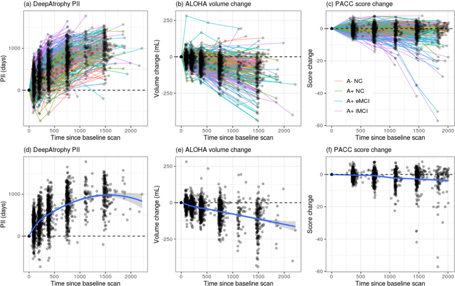
Comparison of (a) DeepAtrophy predicted interscan interval (PII), (b) Automatic Longitudinal Hippocampal Atrophy software/package (ALOHA) volume change, and (c) Preclinical Alzheimer’s Cognitive Composite (PACC) score change for individual subjects for all available scans. For DeepAtrophy, the predicted interscan interval, as an indicator of brain change, is expected to be above zero. For ALOHA and PACC, the volume/score change is expected to be below zero to represent brain atrophy/cognitive decline. Abbreviations: A+/A− = beta-amyloid positive/negative; NC = cognitively normal adults; eMCI = early mild cognitive impairment; lMCI = late mild cognitive impairment.
In order to make the output values of Dθ sensitive not only to the direction of time-related change but also to the magnitude of this change, we modify our training setup and introduce an additional loss function that takes into account the magnitude of the time interval between scans, but in a way that does not depend on the individual subjects’ rates of change. We make a second assumption, that for an individual subject s with three longitudinal scans , , , specified in chronological order , the amount of change between and is greater than the amount of change between and as well as between and . We make a stronger assumption that within a given subject, the amount of change between two timepoints is approximately proportional to the inter-scan interval, i.e.,
We emphasize that the function “change” is used here informally, to denote time-related changes in the images, and is not something that can be measured directly. In practice, this assumption may be violated since disease progression may accelerate or decelerate over time. Nonetheless, much change between scans in year 2 and year 0 of a study than between scans in year 1 and year 0.
To sensitize Dθ to the amount of change between its inputs, we create a new “super-network” Sθ,ω that encompasses two copies of the network Dθ with shared weights and takes two pairs of same-subject scans as inputs (Fig. 1). The network Sθ,ω has the form
where denotes a fully connected layer with weights ω, and denotes the vector concatenation operation. The two pairs of inputs , and , are selected such that and/or and so that one interscan interval contains the other, i.e., or . Note that in most cases, the two pairs are formed by only three distinct scans, e.g., for a subject with scans in 2010, 2011 and 2013, the two pairs may be (2010, 2013) and (2013, 2011). The network is trained using a new categorical loss function, called the relative inter-scan interval (RISI) loss, which is a cross-entropy loss with m classes.1 These classes correspond to different ranges for the ratio of interscan intervals . In our experiments, we use m = 4 classes, corresponding to the ranges [0, 0.5), [0.5, 1), [1, 2), [2, + ∞). The overall expression for our network training has the form
where cat(r) is a function that maps the continuous ratio r to one of the four categorical ranges defined above; and λ is a scalar weight. The first two cross-entropy (ξ) terms above represent the STO loss being computed simultaneously for pairs , and , ; and the last cross-entropy expression represents the RISI loss.
Fig. 1.

Diagram of the DeepAtrophy deep learning algorithm for quantifying progressive change in longitudinal MRI scans. During training, DeepAtrophy consists of two copies of the same “basic sub-network” (Dθ) with shared weights θ. Dθ is a 3D ResNet image classification network with 50 layers (Chen et al., 2019; He et al., 2015) and the output layer having k = 5 elements. Dθ takes as input two MRI scans from the same individual in arbitrary temporal order. The outputs from the two copies of Dθ feed into a 2k × m fully connected layer with weights ω. The resulting “super-network” Sθ,ω, takes as input two pairs of same-subject images, in arbitrary order, and with constraint that the inter-scan interval of one scan pair contains the inter-scan interval of the other scan pair. DeepAtrophy minimizes a weighted sum of two loss functions: the scan temporal order (STO) loss, which measures the ability of Dθ to correctly infer the temporal order of the two input scans; and the relative interscan interval (RISI) loss, which measures the ability of the super-network Sθ,ω, to infer which of the input scan pairs has a longer inter-scan interval. During testing, network Dθ is applied to pairs of same-subject scans. A single measure of disease progression, the predicted interscan interval (PII), is computed as a linear combination of the k outputs of Dθ. The coefficients of this linear combination are obtained by fitting a linear model on the subset of the training data (amyloid negative normal control group) with actual inter-scan interval as the dependent variable and outputs of Dθ as independent variables.
Formulating the problem of interscan interval ratio inference as a classification problem with the four categories above, as opposed to a regression problem, is driven by two considerations. On the one hand, we empirically found the networks with the regression loss much more difficult to train. On the other hand, although we expect the relationship between the relative inter-scan interval and the relative amount of time-related change between image pairs of most subjects to be approximately linear, it may not be case for every individual. The categorical loss allows more deviation from the linearity assumption that potentially fits the actual change trajectory of individual subjects better.
We emphasize that the objective of training the super-network Sθ,ω with the STO and RISI losses is to coerce the network Dθ to output activation values that capture both the directionality (STO loss) and magnitude (RISI loss) of the change between its two input images. The super-network is only used during training. At test time, only the network Dθ is evaluated. This is because at test time, and for application as a longitudinal biomarker, our goal is to generate measures of change for pairs of same-subject images, whereas Sθ,ω requires three or more images from the same subject. While it may be possible to improve the accuracy of Sθ,ω by formulating it as an end-to-end network instead of the current Siamese-like architecture (Bertinetto et al., 2016) with two copies of the network Dθ, doing so would no longer provide us with a network that can measure the amount of time-related change between a pair of input scans.
2.3. Implementation notes
In our implementation, Dθ is based on the ResNet50 deep residual learning network ( He et al., 2015), which is used extensively for image classification in computer vision. We used a 3D version of ResNet50 pre-trained on medical images of multiple organs (not including ADNI data) named MedicalNet ( Chen et al., 2019). We chose the 50-layer ResNet architecture to avoid under- and over-fitting, which occurred in our preliminary experiments when the 18 or 101-layer architectures were used. Experiments were conducted on a Titan 2080 Ti GPU with 8 GB memory. DeepAtrophy training used the learning rate of 0.001, batch size of 15, with 8 epochs, resulting in ~40 h of computation. At each epoch, all available combinations of scan pairs (∼180,000) as described for the RISI loss was input to the network only once.
The number of outputs in the last layer of Dθ was set to k = 5, with the first two outputs passed in as input to the STO loss,2 and all five outputs being used for the computation of the RISI loss. This hyperparameter was set on an ad hoc basis; however, we conducted post hoc experiments with different values of k, which confirmed that the overall network accuracy for our choice (k = 5) was not inferior to a range of other values examined (Supplemental Section S8).
Higher weighting of the RISI loss (λ parameter) encourages the network to focus more effort on detecting the magnitude of disease progression, while higher weighting of the STO loss encourages it to focus more effort on detecting the presence/direction of progression. We chose the weight λ = 1 after conducting preliminary experiments on a random train/test split of the ADNI data and training Sθ,ω with different weights (λ = 0, 0.1, 1, and 10). These preliminary experiments demonstrated that lower values of λ (0, 0.1) resulted in slightly greater accuracy of scan temporal order prediction, but also lower sensitivity to magnitude of change; conversely, a high value of λ (10) resulted in relatively poor scan order inference (Supplemental Section S7) and λ = 1 was chosen as a compromise value.
To avoid any possible bias related to preprocessing, we randomly choose for each scan pair the preprocessing result where the first image in the pair was used as the fixed image during registration or the preprocessing result where the second image was the fixed image.
2.4. Predicted-to-actual interscan interval ratio (PAIIR)
DBM and BSI methods yield intuitive quantitative measures, such as annualized loss of hippocampal volume, that can serve as disease progression and treatment response biomarkers for clinical trials. In this section, we devise a similar quantitative measure of time-related change for DeepAtrophy. We follow the example of recent brain-age prediction studies (Cole and Franke, 2017; Liem et al., 2016), in which the mismatch between a person’s actual age and their “brain age” predicted from neuroimaging and/or other biomarkers is used to characterize individuals in terms of resilience vs. vulnerability to the aging process. Analogously, we define the mismatch between the actual interval between two longitudinal scans and the inter-scan interval inferred by DeepAtrophy as a candidate measure of disease progression. Consider two individuals, one with advanced neurodegenerative disease and the other a healthy older adult, who both have longitudinal scans with inter-scan interval Δt. The first individual will likely experience a greater amount of neurodegeneration over this time than the second, which will be reflected in the longitudinal scans. If DeepAtrophy is sensitive in detecting the presence of time-related change in the input scans, we would expect the output of Dθ for the first individual to reflect a greater amount of change than for the second individual. However, since the output of Dθ is a k-component vector, we must first transform this vector into a scalar measure of apparent time-related change. We do so by fitting a linear model on a subset A− NC individuals in the training set, with each pair of scans , treated as an independent observation, the k components of treated as independent variables, and the actual interscan interval treated as the dependent variable:
where ε is a normal random variable with mean zero. When fitting this model, we consider scan pairs in arbitrary temporal order, so may be positive or negative. For each cross-validation fold, the least squared fit of the model to the data is computed using ∼4600 scan pairs from the A− NC subset of the training set. At test time, we define the predicted interscan interval (PII) for a pair of scans , for subject s′ as
Intuitively, PII is a measure of expected interval between a pair of scans, under the assumption that the subject is from the A− NC cohort. For a subject from this cohort, we would expect that, on average, PII and the actual interscan interval would be equal. For subjects with more advanced disease, we would expect more disease progression over the same time interval than in the A− NC cohort, and we would expect PII on average to be greater than the actual interscan interval. We can define the mismatch between PII and actual inter-scan interval as the predicted-to-actual inter-scan ratio (PAIIR):
We evaluate the suitability of PAIIR as marker of the rate of disease progression and as a surrogate to the conventional DBM-based atrophy rate measurements. PAIIR values larger than one are suggestive of disease progression occurring faster than what is expected for the A− NC group, and we expect PAIIR to be greater on average in patients in more advanced stages of AD.
2.5. Statistical tests
Experiments used a five-fold cross-validation design. The full set of subjects was divided into five approximately equal size subsets (“folds”) and DeepAtrophy training was repeated five times. The folds were stratified across diagnostic groups, i.e., each fold contained approximately 1/5 of the subjects in each group. In each of the training experiments, one fold was held out as the test set and the remaining subjects were included in the training set, with the exception of subjects who only had two longitudinal scans (since DeepAtrophy training requires at least three scans per subject). Measures of accuracy are averaged across the five folds. The number of individuals per group in the training and test sets for each fold are shown in Supplemental Table S1.
In the first set of experiments, we compared the accuracy of temporal ordering of scan pairs (explicitly maximized by the STO loss) and the accuracy of longer vs. shorter interscan interval detection for pairs of scan pairs (explicitly maximized by the RISI loss) between DeepAtrophy and ALOHA. For brevity, we refer to these measures as “STO accuracy” and “RISI accuracy”. Accuracy was computed as the proportion of correct classifications across all scan pairs in the test subsets of the five cross-validation folds. DeepAtrophy (Dθ) and ALOHA were applied to the same set of scan pairs. STO accuracy for DeepAtrophy was computed by comparing the predicted class in the STO loss to the actual scan ordering. STO accuracy for ALOHA was computed by comparing the sign of the annualized hippocampal volume change measure to the scan temporal ordering (i.e., expecting ALOHA to report negative atrophy for a pair of scans in correct temporal order). RISI accuracy for DeepAtrophy was calculated by comparing the PIIs and the actual interscan intervals of two pairs of scans and determining if the scan pair with the larger PII also had the larger actual interscan interval. For ALOHA, the RISI accuracy was calculated by measuring total hippocampal volume change for each scan pair and determining whether the scan pair with the larger absolute value of volume change had a longer interscan interval. STO accuracy for DeepAtrophy and ALOHA is reported as the area under the receiver operating characteristic curve (AUC). To test for the significance in the difference between AUCs of the two methods, DeLong’s test was performed with the R package “pROC” (Robin et al., 2011).
In the second set of experiments, we evaluated the suitability of the PAIIR measure as a biomarker of disease progression by comparing PAIIR between cohorts at different stages of the AD continuum. This is similar to how the suitability of DBM-derived atrophy rate measures is evaluated in the literature (Cash et al., 2015; Fox et al., 2011). We compared effect sizes for group comparisons between A+ NC, A+ eMCI and A+ lMCI groups and the A− NC group, respectively, obtained using PAIIR to the corresponding effect sizes obtained using ALOHA annualized hippocampal volume change measures. In addition, we compared our longitudinal measurements with longitudinal Preclinical Alzheimer’s Cognitive Composite (PACC) score, a standard cognitive test crafted specifically for detecting subtle changes in pre-symptomatic disease (Donohue et al., 2014). These comparative analyses were carried out in two hypothetical scenarios: a one-year clinical trial and a two-year clinical trial. For the one-year scenario, we consider for each subject their baseline scan and all available follow-up scans between 180 and 400 days from baseline. For the two-year scenario, we consider the baseline scan and all available follow-up scans between 400 and 800 days from baseline.
Group difference statistics for DeepAtrophy are computed by pooling the subjects across the five cross-validation folds. Thus, for a given subject s, the PII measurements are obtained by applying the DeepAtrophy network trained on the four folds that do not contain subject s. Likewise, the linear fitting parameters β are estimated using A− NC subjects from the four folds that do not contain subject s. This pooling allows us to maximize the amount of data available for group comparisons, while ensuring clean separation between training and test subsets for each deep learning network and each linear model.
When performing group analyses, each subject was represented by a single summary measure of disease progression, regardless of the number of scans available in the one-year (180–400 days) or two-year (400–800 days) hypothetical scenario. For subjects who had more than two scans (or PACC scores) available, we computed summary measures as follows. For ALOHA, we used the baseline hippocampal volume from ASHS-T1 and pairwise volume change measures between the baseline image and each follow-up image to estimate the hippocampal volume at each time point and fitted a linear model to these measurements. The slope of the linear fit was taken as the summary atrophy measure. For DeepAtrophy, we followed a similar approach, using PII instead of volume change, and using zero for the baseline measurement. For PACC, we also followed this linear fitting approach, however, most subjects had only two tests within the 400-day interval. Additionally, all summary scores (DeepAtrophy, ALOHA, PACC) were corrected for age (at the time of the baseline scan) by fitting a linear model using all subjects and retaining the residual values from the fitted model, similar to Xie et al. (2020b). For each of the above approaches, we conducted the nonparametric Wilcoxon signed-rank test (one-sided, unpaired) between the corresponding measure of disease progression in each disease group (A+ NC, A+ eMCI, and A+ lMCI) and the A− NC group.
Additionally, for DeepAtrophy and ALOHA, we estimated the minimum sample size required to detect a 25%/year and 50%/year reduction in the atrophy rate of each disease stage (A+ NC, A+ eMCI, and A+ lMCI) relative to the to the mean atrophy rate of the A− NC group in a hypothetical clinical trial. This calculation envisions a clinical trial in which participants are patients at a given disease stage (e.g., preclinical AD) and the intervention successfully slows disease progression by 25% or 50% relative to “normal” brain atrophy in this age group (Fox et al., 2011). The sample size describes the minimal number of participants in the treatment and placebo arms of the clinical trial needed to detect a significant difference between the two arms with a two-sided significance level α = 0.05 and power 1-β = 0.8. The sample size is calculated as
where and are the sample means of the patient and control group, and SPAT is the sample standard deviation of the patient group. The 95% confidence interval for each sample size measurement was computed with the bootstrap method (Efron, 1979).
3. Results
3.1. Scan temporal order (STO) inference accuracy
Table 2 reports the mean accuracy of detecting the correct temporal order of a single pair of same-subject scans (STO accuracy) for DeepAtrophy and ALOHA algorithms. Accuracy is averaged across the five cross-validation folds. For each fold, all scan pairs available in the test subset were included in the evaluation (∼4000 scan pairs per fold), with no cutoff for the interscan interval. The scan pairs were supplied to the algorithms in random temporal order. The same set of pairs was evaluated by DeepAtrophy and ALOHA. Overall, the average STO accuracy for DeepAtrophy was 88.5% across all scan pairs in all five folds, compared to 75.5% for ALOHA. For both methods, STO accuracy was lower for less impaired groups, as would be expected since there is less underlying biological change for the same time interval than in more impaired groups. The receiver operating characteristic (ROC) plot in Fig. 2 further contrasts the ability of DeepAtrophy and ALOHA in inferring scan temporal order. For each individual diagnostic group, the area under the curve (AUC) for DeepAtrophy is significantly higher than for ALOHA (p-value < 2.2e-16, the smallest positive number distinguishable from zero in computers).
Table 2.
Average accuracy of the DeepAtrophy PAIIR measure and the ALOHA (Das et al., 2012) hippocampal atrophy rate measure in inferring the scan temporal order (STO) of same-subject scan pairs input in arbitrary order (STO accuracy). For the ALOHA measure, we consider it to be “correct” if the sign of hippocampal atrophy is negative for scans input in chronological order, and positive for scans in reverse chronological order. Accuracy is pooled across all five cross-validation folds. Accuracy is expected to be lower for less impaired groups because there is less underlying biological change for the same time interval than in more impaired groups. Abbreviations: ALOHA = Automatic Longitudinal Hippocampal Atrophy software/package; A+/A− = beta-amyloid positive/negative; NC = cognitively normal adults; eMCI = early mild cognitive impairment; lMCI = late mild cognitive impair.
| A− NC | A+ NC | A+ eMCI | A+ lMCI | All Groups | |
|---|---|---|---|---|---|
| ALOHA | 69.7% | 74.3% | 75.1% | 85.2% | 75.5% |
| DeepAtrophy | 85.4% | 89.5% | 88.6% | 92.4% | 88.5% |
Fig. 2.
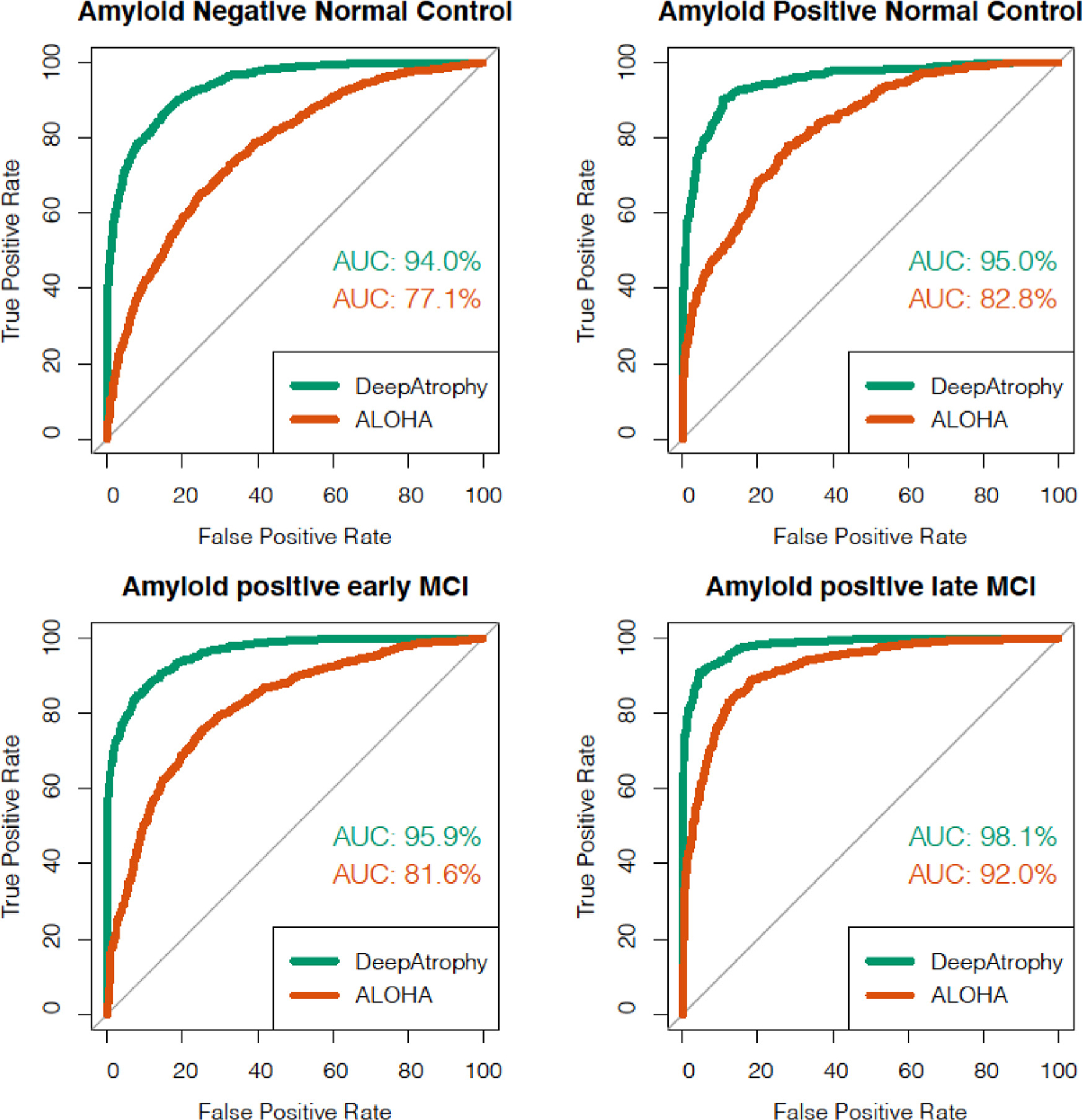
Area under the receiver operating characteristic (ROC) curve (AUC) for the scan temporal order (STO) inference experiments using DeepAtrophy and ALOHA, pooled across test subsets of the five cross-validation folds. Greater AUC for DeepAtrophy indicates greater accuracy in inferring the temporal order of scans. Abbreviations: ALOHA = Automatic Longitudinal Hippocampal Atrophy software/package; MCI = mild cognitive impairment; AD = Alzheimer’s Disease.
3.2. Relative inter-scan interval (RISI) inference accuracy
Table 3 compares the mean accuracy of DeepAtrophy and ALOHA in the task of inferring which out of two pairs of same-subject scans has a longer interscan interval (RISI accuracy). This evaluation used data from all subjects in the five folds who had at least three scans, with no maximum cutoff for the interscan interval. The two approaches were applied to the same set of input scans. DeepAtrophy has higher RISI accuracy (81.1%) compared with ALOHA (75.0%). This suggests that deep learning can infer not only the presence, but also the magnitude of disease progression from a pair of MRI scans. Similarly, Fig. 3 shows the ROC curve in the ability of DeepAtrophy and ALOHA in inferring relative interscan interval. For A− NC, A+ NC and A+eMCI groups, the AUC of DeepAtrophy is significantly higher than that of ALOHA (p-value < 2.2e-16). For A+ lMCI group, there is no significant difference (p = 0.69) between ALOHA and DeepAtrophy in the AUC value.
Table 3.
Comparison of relative inter-scan interval (RISI) inference accuracy for DeepAtrophy and ALOHA. Given two pairs of scans from the same subject of different interscan-intervals, a method sensitive to underlying biological change should be able to correctly detect which scan pair has a longer inter-scan interval. Abbreviations: ALOHA = Automatic Longitudinal Hippocampal Atrophy software/package; A+/A− = beta-amyloid positive/negative; NC = cognitively normal adults; eMCI = early mild cognitive impairment; lMCI = late mild cognitive impairment.
| A− NC | A+ NC | A+ eMCI | A+ lMCI | All Groups | |
|---|---|---|---|---|---|
| ALOHA | 68.8% | 72.7% | 76.3% | 83.4% | 75.0% |
| DeepAtrophy | 79.3% | 81.5% | 81.3% | 83.3% | 81.1% |
Fig. 3.
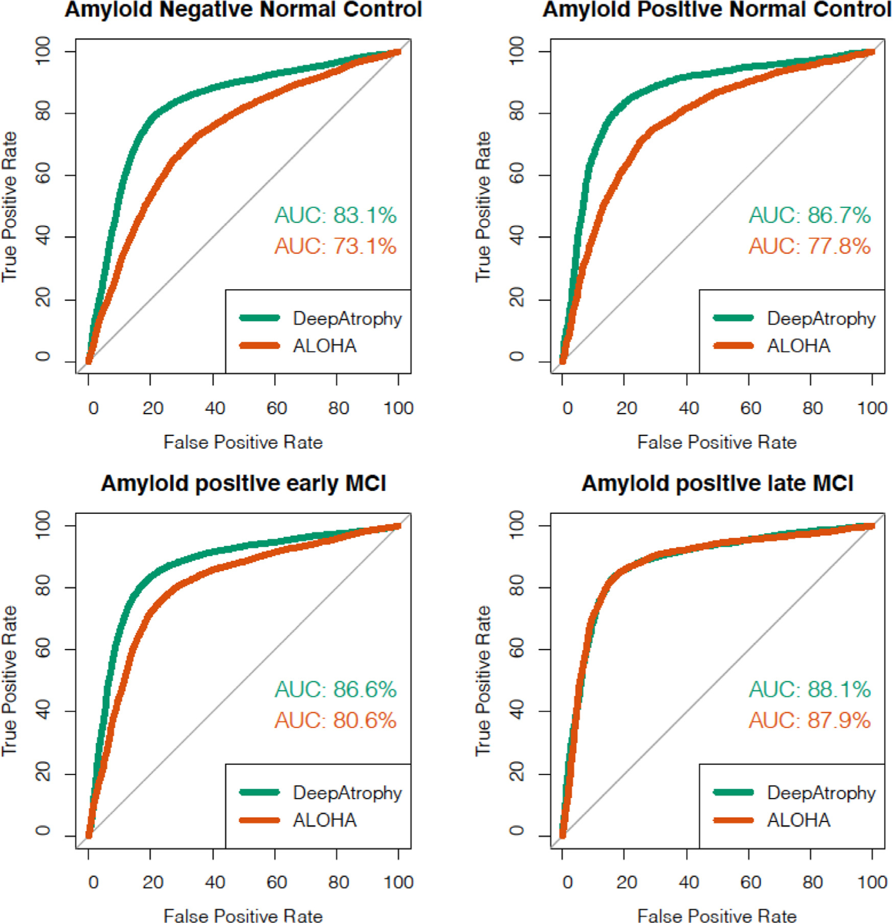
Area under the receiver operating characteristic (ROC) curve (AUC) for the relative interscan interval (RISI) inference experiments using DeepAtrophy and ALOHA, pooled across test subsets of the five cross-validation folds. Greater AUC for DeepAtrophy indicates greater accuracy in inferring which pair of scans has a longer acquisition time interval. Abbreviations: ALOHA = Automatic Longitudinal Hippocampal Atrophy software/package; MCI = mild cognitive impairment; AD = Alzheimer’s disease.
3.3. Visualizing disease progression in individual subjects
Fig. 4 uses spaghetti plots to visualize the trajectories of DeepAtrophy, ALOHA and PACC disease progression measures for individual subjects for all scan times. The plots are pooled across all five cross-validation folds. For each subject and each method, the plot shows the corresponding measure (PII for DeepAtrophy, hippocampal volume change for ALOHA, score difference for PACC) between the baseline scan and each follow-up scan. For DeepAtrophy, the progression measure should increase with time (since the PII is expected to be consistent with the actual interscan interval), whereas for ALOHA and PACC, the progression measure (hippocampal volume, PACC score) is expected to decrease with time. Moreover, we expect the relationship between time interval and each progression measure to be approximately linear, in aggregate. While it is common to model tissue loss as an exponential decay process (Wagner et al., 2008), at the rates expected in the ADNI cohort (0.5% to 4% a year), the relationship is approximately linear. Indeed, for ALOHA, we observe a close to linear relationship overall, although there is a great deal of variation among the individual trajectories. Reflecting the lower STO accuracy of ALOHA, a number of trajectories are in the upper quadrant of the coordinate space, which corresponds to increasing hippocampal volume over time. In contrast, the trajectories of DeepAtrophy are almost entirely in the upper right quartile (consistent with its high STO accuracy), but the relationship between the predicted interscan interval and time is sublinear, i.e., exhibiting diminishing returns with respect to time, suggesting that DeepAtrophy is sensitized to short-term longitudinal changes to a greater extent than to longer-term changes. Notably, when the weight of the RISI loss in DeepAtrophy is reduced (shown in spaghetti plots in Supplemental Figure S2), the relationship becomes even less linear, with PII underestimating the actual inter-scan interval for longer inter-scan intervals. The diminishing returns observed in the spaghetti plots for PII, especially for low values of λ, is much more pronounced than what might be reasonably explained by disease progression following an exponential model at rates of 0.5% to 4% a year. This highlights the importance of the RISI loss in teaching the network to detect not just the directionality of time-related changes between longitudinal scans, but also its magnitude. The trajectories for PACC are much noisier than that of the MRI-based measures. For all three measurements, individuals with more severe disease tend to have trajectories with a higher slope than healthier individuals, suggesting that all three measurements can differentiate differences in the rates of disease progression across the spectrum of AD.
3.4. Group differences in rates of disease progression
In the remaining experiments, we compare the measures of disease progression generated by DeepAtrophy, ALOHA and PACC between groups of ADNI participants at different stages of the AD continuum. The three “disease” groups, i.e., preclinical AD (A+ NC), early prodromal AD (A+ eMCI) and late prodromal AD (A+ lMCI), are compared to the “control” group (A− NC) using each of the measures. The group analyses are performed by pooling together the subjects across the five cross-validation folds, as described in Section 2.5. Fig. 5a plots the distribution of DeepAtrophy, ALOHA, and PACC disease progression measures for the four groups in the one-year hypothetical clinical trial scenario (scans between 180 and 400 days from baseline) and identifies statistically significant group differences with the control group. For all three measures, the average measure of progression increases with disease severity. DeepAtrophy detects a difference between preclinical AD and the control group that is borderline significant (p = 0.022, one-alternative Wilcoxon rank-sum test, uncorrected). For early and late prodromal AD, both DeepAtrophy and ALOHA detect statistically significant differences relative to the control group (p-value < 0.001, one-alternative Wilcoxon test, uncorrected). Unlike the MRI-based measures, with PACC, only the difference between A+ lMCI and controls is significant for the one-year scenario. Analogous results for the two-year clinical trial scenario are presented in Fig. 5b. Here, both DeepAtrophy and ALOHA detected differences between preclinical AD and controls (p = 0.011 for DeepAtrophy, p = 0.0061 for ALOHA, one-alternative Wilcoxon test, uncorrected), with the p-value smaller in absolute terms for ALOHA. Both methods detected significant differences with A− NC in the prodromal MCI groups. Supplemental Figure S1 plots the ROC curves using DeepAtrophy and ALOHA measures for separation between each patient group and the control group. Within each disease group, the ROC curves for DeepAtrophy and ALOHA are very close to each other and AUCs are not statistically different between the methods. Overall, the group separation results do not allow us to conclude that either DeepAtrophy or ALOHA is a “better” longitudinal biomarker than the other, indeed the two measures appear quite comparable to each other.
Fig. 5.
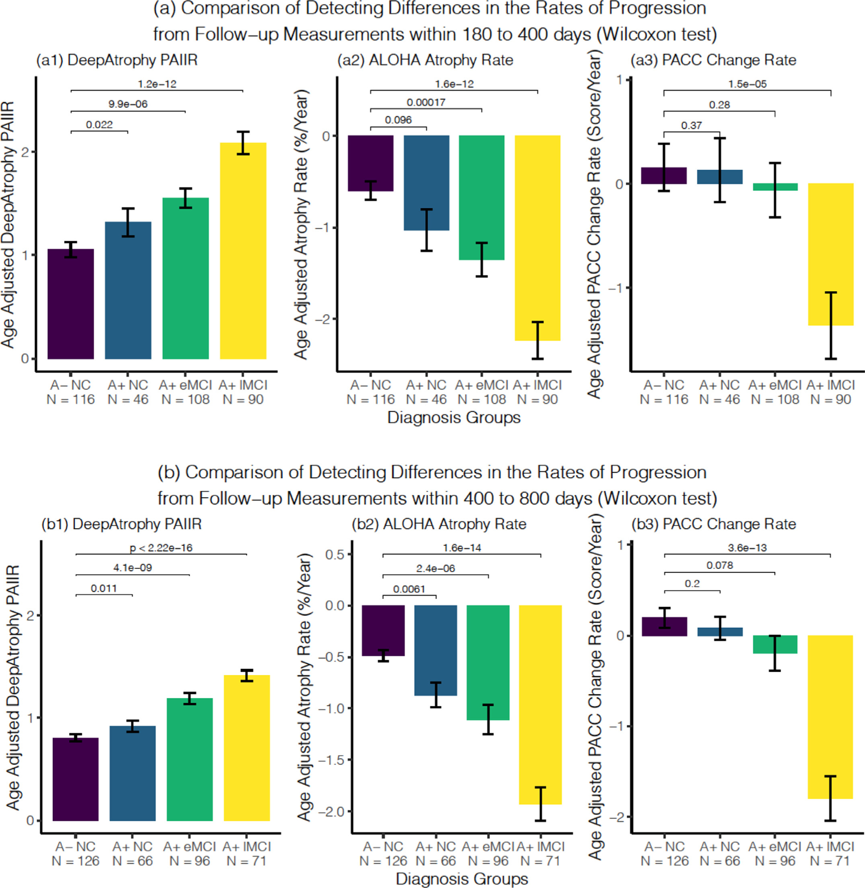
Comparison of the ability of DeepAtrophy PAIIR measure, ALOHA atrophy rate, and PACC score change rate to detect differences in the rates of disease progression between normal controls (A− NC) and three disease groups: preclinical AD (A+ NC), early prodromal AD (A+ eMCI) and late prodromal AD (A+ lMCI) using follow-up timepoints between (a) 180 to 400 days from baseline (one-year clinical trial scenario) and (b) 400 to 800 days from baseline (two-year clinical trial scenario). In each subplot, the Wilcoxon signed-rank test was conducted to compare each patient group with the control group, and the p-values were shown for each comparison. Abbreviations: PAIIR = predicted-to-actual interscan interval ratio; ALOHA = Automatic Longitudinal Hippocampal Atrophy software/package; PACC = Preclinical Alzheimer’s Cognitive Composite; A+/A− = beta-amyloid positive/negative; NC = cognitively normal adults; eMCI = early mild cognitive impairment; lMCI = late mild cognitive impairment; N = number of subjects in the diagnosis group.
3.5. Sample size estimation for a hypothetical clinical trial
Table 4 presents sample size estimates (and 95% confidence intervals) for different hypothetical clinical trial scenarios using either DeepAtrophy, ALOHA or PACC to track disease progression. Different clinical trial scenarios include participants with different severity of AD (preclinical AD, early prodromal AD, late prodromal AD), different duration (1 vs. 2 years), and different expected reduction in rate of disease progression (25% vs. 50%) in trial participants receiving treatment. As described in Section 2.5, the reduction is computed relative to the rate of progression in controls. In all scenarios, the sample size calculation is based on the statistics (mean and variance) of the four diagnosis groups plotted in Fig. 5. For all A+ eMCI and A+ lMCI scenarios, DeepAtrophy is associated with a smaller sample size estimate (in absolute terms) than ALOHA, although 95% confidence intervals overlap. Conversely, for preclinical AD scenarios, the sample size estimates for ALOHA are smaller than or similar to DeepAtrophy. This might be explained by a stronger variance in the A− NC group in DeepAtrophy, which may lead to higher sample size estimates. In all cases, the 95% confidence intervals significantly overlap between DeepAtrophy and ALOHA sample size estimates, so it is not possible to conclude that one set of estimates is statistically better than the other.
Table 4.
Sample size estimates (and 95% confidence intervals in parentheses) to power a one-year or two-year clinical trial to detect a 25%/year or 50%/year reduction (relative to A− NC) in the rate of disease progression of each patient group. See Section 2.5 for the sample size calculation. Measurements with a smaller sample size estimates (in absolute terms) are highlighted in bold. Abbreviations: ALOHA= Automatic Longitudinal Hippocampal Atrophy software/package; A+/A− = beta-amyloid positive/negative; NC = cognitively normal adults; eMCI = early mild cognitive impairment; lMCI = late mild cognitive impairment; 1M = 1,000,000.
| 1-year trial (180 to 400 days) | 2-year trial (400 to 800 days) | ||||
|---|---|---|---|---|---|
| 25% reduction | 50% reduction | 25% reduction | 50% reduction | ||
| A+ NC | DeepAtrophy | 3075 (574, 899,750) | 769 (146, 284,814) | 3597 (681, 764,563) | 900 (169, 90,163) |
| ALOHA | 3175 (778, 524,672) | 794 (190, 108,735) | 1657 (683, 13,580) | 415 (167, 3173) | |
| PACC | 1,658,058 (443,577, > 1M) | 414,515 (100,466, > 1M) | 21,758 (1998, > 1 M) | 5440 (495, > 1M) | |
| A+ eMCI | DeepAtrophy | 914 (422, 3400) | 229 (107, 828) | 485 (256, 1178) | 122 (64, 298) |
| ALOHA | 1575 (652, 7672) | 394 (169, 2288) | 1322 (555, 8372) | 331 (134, 1880) | |
| PACC | 38,395 (3781, > 1M) | 9599 (912, > 1M) | 5888 (1371, > 1M) | 1472 (329, 232,773) | |
| A+ lMCI | DeepAtrophy | 251 (156, 464) | 63 (38, 112) | 129 (80, 231) | 33 (21, 59) |
| ALOHA | 327 (192, 703) | 82 (48, 176) | 218 (129, 420) | 55 (32, 104) | |
| PACC | 988 (413, 4688) | 247 (102, 1140) | 267 (149, 631) | 67 (37, 158) | |
4. Discussion
In this paper, we considered the problem of quantifying change from longitudinal MRI scans in the context of neurodegenerative disease. The leading solutions to this problem (DBM, BSI) involve using some form of image registration to compare scans to each other and deriving a measure of expansion or contraction in relevant to anatomical structures, e.g., the hippocampus. Such registration-based measures are very sensitive to small shifts in anatomical boundaries caused by progressive neurodegeneration. However, they may also misinterpret imaging artifacts, such as those caused by subject motion, as atrophy. The relatively high fraction of positive atrophy values (i.e., hippocampal volume increasing over time) reported by the state-of-the-art DBM method ALOHA (25% in our dataset) is suggestive of imaging artifacts influencing conventional longitudinal measures.
We set out to design a deep learning approach that would serve as an alternative to conventional registration-based longitudinal analysis techniques. Deep learning usually relies on large training datasets, yet in this problem, the ground truth is unknown, i.e., the true amount of disease-related change between pairs of MRI scans cannot be estimated by practical means. Instead, we trained our networks to infer temporal information from longitudinal scan pairs, under the assumption that differences between images that are correlated with the passing of time are primarily caused by aging and disease progression. If this assumption is true, then a network trained to infer scan temporal order and relative interscan interval is likely implicitly learning to detect aging and disease progression. By using relative measures of time when training the neural network, rather than absolute ones (i.e., using STO and RISI losses instead of directly inferring PII from scan pairs), our approach implicitly accounts for different rates of disease progression in different individuals.
Our results in Tables 2 and 3 show that DeepAtrophy can be taught to temporally order scans and detect shorter vs. longer inter-scan intervals with significantly greater accuracy than ALOHA. This suggests that longitudinal scans encompass information about time-related changes that goes well beyond what is captured by the displacement of hippocampal boundaries. We did not compare DeepAtrophy with other conventional techniques, but recent studies (Cash et al., 2015; Das et al., 2012; Xie et al., 2020a) suggest that ALOHA performs on par with other leading DBM (Lorenzi et al., 2015a) and BSI techniques (Freeborough and Fox, 1997; Leung et al., 2010). For both DeepAtrophy and ALOHA, temporal inference accuracy in Tables 2 and 3 generally increases with disease severity, which is to be expected, since the magnitude of the expected change in image content is greater in groups that experience higher rates of neurodegeneration. Increased sensitivity of the longitudinal measure and lower frequency of positive atrophy values (i.e., reports of hippocampal volume increase) in more affected groups is consistent with other atrophy measurement methods (Hua et al., 2016; Leung et al., 2010; Yushkevich et al., 2009).
One critical question is whether the high temporal inference accuracy in DeepAtrophy reflects greater sensitivity to progressive biological changes (i.e., neurodegeneration), or whether other non-biological factors that are not independent of time are present. For example, in a single-site longitudinal study, a change in scanner hardware or protocol parameters at certain points over the duration of the study would result in differences in image content that are systematic with respect to time, yet not biological (e.g., scans acquired later in the study might have better gray/white tissue contrast). A CNN could easily detect this difference, resulting in high temporal inference accuracy. However, in such a scenario, we would expect the STO accuracy of the CNN to be high, but less so the RISI accuracy. Most importantly, if such a CNN was primarily detecting factors that are systematic but non-biological, we would not expect to observe significant differences in CNN output between less affected and more affected individuals. The fact that DeepAtrophy has high RISI accuracy (Table 3), performs on par with ALOHA at group separation (Fig. 5), and is trained on a multi-site multi-scanner dataset, makes it unlikely that systematic non-biological factors are driving its temporal inference accuracy. In future work, it would be informative to relate data on software and hardware changes at ADNI sites during the ADNI2/GO phases the study to DeepAtrophy measures, and thus determine to what extent these measures are impacted by these systematic but non-biological changes.
Inconsistent preprocessing of MRI scans input to DeepAtrophy could provide another possible explanation of high temporal accuracy reported in Tables 2 and 3. However, we took great care to make sure all scans underwent the same preprocessing, i.e., performing rigid registration in half-way space (Das et al., 2012; Yushkevich et al., 2009) and randomly assigning the roles of “fixed” and “moving” image in registration. Additionally, in the Supplemental Section S2, we tested DeepAtrophy on nine subjects scanned on the same day. The STO accuracy in this experiment was close to 50%, i.e., close to chance, which likely rules out the possibility of preprocessing differences contributing to high temporal inference accuracy of DeepAtrophy.
We introduced a scalar measure of mismatch between the inter-scan interval inferred by DeepAtrophy from a pair of scans and the actual inter-scan interval (PAIIR) as a potential biomarker for tracking disease progression in AD clinical trials. PAIIR was envisioned as an analogue to conventional biomarkers like hippocampal atrophy rate in DBM. However, we found that differences in the age-adjusted PAIIR measure between amyloid-negative controls and patients at different stages of the AD continuum were on par with the differences in the age-adjusted ALOHA hippocampal atrophy measure (Fig. 5, Table 4, and Supplemental Figure S1), i.e., no statistically significant differences were detected between the two measures in the ROC analysis, and 95% confidence intervals for the sample size estimates in Table 4 overlapped. It is unclear why DeepAtrophy outperforms ALOHA in terms of STO and RISI accuracy yet does not improve on ALOHA for separating patient groups. One possible explanation is that DeepAtrophy has greater sensitivity to overall progressive change, but ALOHA has greater specificity to disease-related neurodegeneration. Individuals in ADNI may be undergoing simultaneous progressive changes: some related to aging, and some related to disease. For example, all individuals may undergo widespread loss of brain tissue that is systematic but generally unrelated to disease progression. Since DeepAtrophy is not specifically taught to recognize disease-related changes, it may “lock on” the more global systematic changes, which would be sufficient to infer temporal information successfully, but would not be helpful for differentiating groups at different stages of AD. By contrast, ALOHA measures change in the hippocampus, a brain structure more specifically linked to neurodegenerative diseases. Hence, ALOHA may be less sensitive to time-related change (hence lower STO/RISI accuracy) but more attuned to disease-related differences in progression. It is conceivable that a strategy that combines deep learning-based time inference with anatomy-informed deformation-based morphometry, i.e., a hybrid DeepAtrophy/ALOHA method, would improve on both ALOHA and DeepAtrophy by boosting the sensitivity of the former and the specificity of the latter.
Indeed, ALOHA and DeepAtrophy appear to provide complementary information for separating groups along the AD continuum. In Supplemental Section S4, we report the results of stepwise logistic regression analysis performed with group (e.g., A+ NC vs A− NC) as the dependent variable, and both ALOHA and DeepAtrophy age-corrected progression measures as independent variables. For analyses involving A+ eMCI and A+ lMCI groups, both ALOHA and DeepAtrophy measures are included in the final model (in both 1-year and 2-year clinical trial scenarios), although for the analysis involving the A+ NC group, only the ALOHA measure is included (in both 1-year and 2-year clinical trial scenarios). This suggests that there is promise in combining DeepAtrophy and ALOHA in a hybrid method.
The overall conclusions of the experiments in this study may be stated as follows: there appears to be time-associated information in longitudinal scan pairs that is untapped by conventional DBM measures but leveraging this information into a more effective AD disease progression biomarker will likely require a hybrid approach that combines explicit image-based time inference (as in DeepAtrophy) with explicit focus on AD-specific brain regions (as in ALOHA).
4.1. Deep learning for AD longitudinal biomarkers
Current deep learning techniques for AD analysis are focused mainly on the diagnosis and prediction of structural change or cognitive scores of AD (Li and Fan, 2019; Parisot et al., 2018; Spasov et al., 2019; Zhang et al., 2017). It includes classification of the future AD stages (Basu et al., 2019) or time of conversion from one state to another (Lee et al., 2019; Lorenzi et al., 2019), and regression of biomarker values, such as cognitive scores and ventricle volumes (Ghazi et al., 2019; Jung et al., 2019). Prediction of AD stage and conversion time were mainly conducted with Recurrent Neural Networks (RNN), including Long-Short Term Memory (LSTM) networks (Ghazi et al., 2019; Lee et al., 2019; Li and Fan, 2019), in which biomarkers collected at each time go through a node of the RNN, and the output of the network in each later node is the prediction score. In the recent TADPOLE challenge (Azvan et al., 2020), the best performing team overall (ventricle volume, diagnosis, and cognitive score prediction) uses XGboost method (Chen and Guestrin, 2016); the best performing team in predicting ventricle volume alone uses data-driven disease progression model and machine learning (linear mixed effect model) (Venkatraghavan et al., 2018). Besides, Generative Adversarial Networks (GAN) have been applied to generate future images with or without AD pathology on the whole brain or in the MTL region (Bowles et al., 2018; Ravi et al., 2019).
To our knowledge, none of the DL longitudinal MRI analysis methods employed deep learning specifically as a means to derive a more effective disease progression and treatment evaluation biomarker for clinical trials for AD. DL-based registration methods in which deformation fields are generated by a convolutional neural network (CNN) are an area of active research (Balakrishnan et al., 2018; Tustison et al., 2019; Yang et al., 2017). However, the impact of these methods on disease progression biomarkers in AD has not yet been evaluated.
4.2. Clinical trial sample size estimates: comparison to the literature
Studies commonly evaluate longitudinal biomarkers in AD by estimating the sample size needed to power a hypothetical clinical trial in which the experimental treatment is expected to reduce the rate of disease progression by 25% relative to the healthy aging (Holland et al., 2012a; Hua et al., 2016; Pegueroles et al., 2017; Yushkevich et al., 2009). Sample size estimates reported in the literature for longitudinal MRI-based biomarkers are generally smaller than for cognitive testing (Ard and Edland, 2011; Cullen et al., 2020; Weiner et al., 2015; Xie et al., 2020b), as we also report in Table 4 for the PACC measure. Most sample size estimates reported in the literature involve hypothetical clinical trials in MCI or AD. In the MIRIAD challenge (Cash et al., 2015), the smallest reported sample sizes for a hypothetic 12 month clinical trial in AD were 190 (95% CI: 146 to 268) and 158 (95% CI: 116 to 228) for left and right hippocampal atrophy rate measures, respectively. In the original report on ALOHA (Das et al., 2012), a sample size of 269 (based on a one-sided test, corresponds to 343 for two-sided) was estimated for a hypothetical one-year trial in MCI (regardless of beta-amyloid status) using a hippocampal volume atrophy measure derived from longitudinal high-resolution T2-weighted MRI; and sample size of 325 (414 two-sided) when using T1-weighted MRI. In a subsequent comparison of FreeSurfer (FS), Quarc, and KN-BSI T1-MRI analysis methods in Holland et al. (2012), the minimum sample size reported for a one-year trial in late MCI was 327 (95% CI: 209 to 585). However, even though the sample size in these studies was reported for a one-year trial, the annualized atrophy rates used to estimate these sample sizes used longitudinal scans with up to three years follow-up. By contrast, in a hypothetical one-year clinical trial in late MCI, the sample size using DeepAtrophy is estimated to be 251 (95% CI: 156 to 464), and unlike the above studies, this estimate is based on one-year follow-up data. The corresponding estimate for ALOHA is 327 (95% CI: 192 to 703). This suggests that DeepAtrophy performs on par with the state-of-the-art conventional methods for disease progression quantification in the context of symptomatic AD.
Compared to MCI/AD, there has been relatively less work on estimating the sample size needed to power a hypothetical clinical trial in preclinical AD. Insel et al. (2019) report a sample size of 2000 for a 4-year clinical trial using PACC as the outcome measure. Holland et al. (2012b) performed sample size estimation for a three-year clinical trial in preclinical AD, where they reported n = 1763 (95% CI: [400, >100,000]) needed to detect a 25% reduction in longitudinal hippocampus change rate relative to controls, applied to data collected in 3 years. However, the sample size estimated for a hypothetical 3-year clinical trial for a 25% reduction in hippocampus volume change by Bertens et al. (2017) is 279 (95% CI: [197, 426]). Xie et al. (2020b) reported the results of the ALOHA analysis described in the current study and reported sample sizes consistent with the results in Table 4.
4.3. Limitations and future work
Perhaps the main limitation of DeepAtrophy compared to DBM/BSI techniques is that it provides a holistic interpretation of change over time in a longitudinal scan pair and does not shed light on neurodegeneration in specific anatomical regions. Whereas ALOHA can provide measures of change in specific anatomical regions (hippocampus, Brodmann area 35), DeepAtrophy yields only a single measure for the hippocampal region. This limits the interpretability of the DeepAtrophy results, which is a common limitation of many deep learning image analysis approaches. However, existing approaches for interpretation of deep learning models (e.g., attention mapping, gradient-based techniques (Selvaraju et al., 2016; Zhang et al., 2018), weakly supervised learning (Durand et al., 2017), or layer-wise relevance propagation (Bach et al., 2015; Eitel et al., 2019)) can be readily applied to DeepAtrophy, and we plan to conduct such analyses in future work.
Another potential limitation of DeepAtrophy is that its response (PII) diminishes for longer time intervals. The individual trajectories of PII plotted in Fig. 4 and Supplemental Figure S7 are non-linear and exhibit diminishing returns over greater time intervals. This is particularly prominent when DeepAtrophy is trained using only the STO loss, in which case, the response of the network to scan pairs with longer interscan intervals is only slightly greater, on average, than for short interscan intervals (Supplemental Figure S2, Panel (a)). Introducing the RISI loss and increasing its weight makes the trajectories more linear, but this comes at the cost of reduced STO accuracy, i.e., there is a tradeoff between accuracy in detecting the presence/directionality of time-related change, and the magnitude of the time-related change. By contrast, the trajectories for the ALOHA hippocampal atrophy rate measure are closer to linear, as would be expected.3 The ability of a biomarker to quantify the magnitude and not just presence of progression is important because in a clinical trial both the treatment and the placebo cohort are expected to have disease progression, and the role of a biomarker is to detect a subtle difference in rates of progression. In this sense, the PII/PAIIR has a lower transitivity than ALOHA measures.
Hyperparameter selection during for DeepAtrophy was performed in a somewhat ad hoc manner. Some parameters (e.g., k, the number of outputs in the last activation layer of Dθ, were assigned ad hoc values and examined post hoc, as reported in Supplemental Section S8, Table S7). Other parameters (e.g., number of training epochs and λ, the weight of the RISI loss) were tuned on a single random training/test split of the full ADNI dataset. A more elegant and statistically robust strategy would have been to optimize the hyperparameters on a held-out validation set. However, given the sparsity of longitudinal MRI data, particularly for preclinical AD, we opted to include all the available participants in the analysis, and to use a cross-validation design, such that DeepAtrophy measures computed for each ADNI subject were derived by training DeepAtrophy on distinct subjects. With additional preclinical AD longitudinal datasets such as the A4 study (Sperling et al., 2014) becoming available in the future, it will be possible to evaluate whether the results reported here generalize to new patient populations, scanners, and protocols. Some of the complexity in terms of hyperparameters was caused by the need to design the RISI loss as a categorical loss, due to the failure of a continuous regression loss to converge during training. Further research, including the modification of the underlying image classification deep network (Xie et al., 2020b), may lead to better trainability of a regression-type RISI loss, in turn reducing the complexity of the training setup and perhaps leading to greater sensitivity to disease progression.
Another limitation of our approach is that it focuses on pairs of scans at test time. When three or more scans are available, we use linear models to infer a summary PAIIR measure from pairwise PAIIR data. Directly incorporating multiple scans into the network, perhaps in a recurrent neural network architecture, may offer additional efficiencies and improved accuracy over the current approach. Lastly, the fact that our experiments are only carried out in a single region of the brain containing the hippocampus and surrounding structures is also a limitation. Additional experiments need to be conducted to determine whether DeepAtrophy can detect time-related changes in other brain regions associated with AD neurodegeneration or at the whole-brain level.
Our future work will focus on addressing these limitations, as well as combining ALOHA and DeepAtrophy in a common algorithmic framework. One potential approach would be to construct a single end-to-end network that implements ALOHA functionality as a set of CNN layers, and to train such a network to generate atrophy measurements that are both faithful to the input data and accurate in terms of temporal inference. The core of ALOHA is diffeomorphic deformable registration, and a number of models for implementing registration as a set of CNN components are available in the literature (Balakrishnan et al., 2018; Tustison et al., 2019; Yang et al., 2017). Such a hybrid network would yield Jacobian determinant maps and region-specific atrophy measures similarly to ALOHA, thus addressing one of the main limitations of DeepAtrophy: its failure to produce anatomically meaningful measures of tissue compression and expansion. However, the registration layers would be sensitized, through the minimization of STO and RISI-like losses, to changes that are systematic with respect to time.
Conclusion
In this paper, we showed that a deep learning network, DeepAtrophy, can infer the temporal order of same-subject longitudinal MRI scans, as well as deduce which pair of same-subject scans has a longer interscan interval, with excellent accuracy, significantly improving on that of a state-of-the-art deformation-based morphometry approach ALOHA. The design of DeepAtrophy encapsulates the underlying assumption that in the context of Alzheimer’s disease, image changes that are systematic with time are primarily related to aging and/or neurodegeneration. We formulated a summary measure of time-associated change between longitudinal MRI scans, defined as the mismatch between the interscan interval predicted by the DeepAtrophy network and the actual inter-scan interval, and showed that this mismatch measure separates cohorts at different stages along the AD continuum comparably to the ALOHA-derived hippocampal atrophy rate measure. Our results suggest that deep learning based temporal inference may capture longitudinal changes that are distinct from those captured by deformation-based morphometry, and that combining both approaches in a hybrid strategy may perhaps lead to a more powerful biomarker for quantifying disease progression in AD clinical trials.
Supplementary Material
Acknowledgment
This work was supported by National Institute of Health (NIH) (Grant Nos R01-AG056014, R01-AG040271, P30 AG072979, R01 AG069474, R01-AG055005), Alzheimer’s Association (AARF-19-615258), and Fondation Philippe Chatrier.
Data collection and sharing for this project was funded by the Alzheimer’s Disease Neuroimaging Initiative (ADNI) (National Institutes of Health Grant U01 AG024904) and DOD ADNI (Department of Defense award number W81XWH-12-2-0012). ADNI is funded by the National Institute on Aging, the National Institute of Biomedical Imaging and Bioengineering, and through generous contributions from the following: AbbVie, Alzheimer’s Association; Alzheimer’s Drug Discovery Foundation; Araclon Biotech; BioClinica, Inc.; Biogen; Bristol-Myers Squibb Company; CereSpir, Inc.; Cogstate; Eisai Inc.; Elan Pharmaceuticals, Inc.; Eli Lilly and Company; EuroImmun; F. Hoffmann-La Roche Ltd and its affiliated company Genentech, Inc.; Fujirebio; GE Healthcare; IXICO Ltd.; Janssen Alzheimer Immunotherapy Research & Development, LLC.; Johnson & Johnson Pharmaceutical Research & Development LLC.; Lumosity; Lundbeck; Merck & Co., Inc.; Meso Scale Diagnostics, LLC.; NeuroRx Research; Neurotrack Technologies; Novartis Pharmaceuticals Corporation; Pfizer Inc.; Piramal Imaging; Servier; Takeda Pharmaceutical Company; and Transition Therapeutics. The Canadian Institutes of Health Research is providing funds to support ADNI clinical sites in Canada. Private sector contributions are facilitated by the Foundation for the National Institutes of Health (www.fnih.org). The grantee organization is the Northern California Institute for Research and Education, and the study is coordinated by the Alzheimer’s Therapeutic Research Institute at the University of Southern California. ADNI data are disseminated by the Laboratory for Neuro Imaging at the University of Southern California.
Footnotes
Credit authorship contribution statement
Mengjin Dong: Methodology, Software, Validation, Formal analysis, Writing – original draft, Visualization. Long Xie: Methodology, Validation, Investigation, Data curation, Resources, Writing – review & editing, Supervision. Sandhitsu R. Das: Methodology, Investigation, Writing – review & editing. Laura E.M. Wisse: Investigation, Data curation. Robin deFlores: Investigation, Data curation. David A. Wolk: Methodology, Investigation, Funding acquisition. Paul A. Yushkevich: Conceptualization, Methodology, Formal analysis, Investigation, Writing – review & editing, Supervision, Project administration, Funding acquisition.
Supplementary materials
Supplementary material associated with this article can be found, in the online version, at doi:10.1016/j.neuroimage.2021.118514.
A continuous loss function, such as the mean square error loss, would in principle be a more natural way to implement RISI. However, in our preliminary experiments, training often failed to converge using continuous losses, while the categorical loss converged consistently.
Note the slight abuse of notation in the expression above, which should be read as the application of the cross-entropy function to the first two elements of the k-component vector .
In theory, trajectory of hippocampal volume in neurogenerative disease would exhibit exponential decay, however at rates reported for the ADNI population (0.5–4% hippocampal volume loss per year (Cash et al., 2015)) and over time intervals examined in this paper, such trajectories can be closely approximated by a linear function.
References
- Ard MC, Edland SD, 2011. Power calculations for clinical trials in Alzheimer’s disease. [DOI] [PMC free article] [PubMed] [Google Scholar]
- Avants BB, Epstein CL, Grossman M, Gee JC, 2007. Symmetric diffeomorphic image registration with cross-correlation: evaluating automated labeling of elderly and neurodegenerative brain. [DOI] [PMC free article] [PubMed] [Google Scholar]
- Azvan R, Marinescu V, Oxtoby NP, Young AL, Bron EE, Toga AW, Weiner MW, Barkhof F, Fox NC, Golland P, Klein S, Alexander DC, 2020. TADPOLE challenge: accurate Alzheimer’s disease prediction through crowdsourced forecasting of future data. [DOI] [PMC free article] [PubMed] [Google Scholar]
- Efron B, 1979. Bootstrap methods: another look at the Jacknife. [Google Scholar]
- Bach S, Binder A, Montavon G, Klauschen F, Müller K-R, Samek W, 2015. On pixel-wise explanations for non-linear classifier decisions by layer-wise relevance propagation. [DOI] [PMC free article] [PubMed] [Google Scholar]
- Balakrishnan G, Zhao A, Sabuncu MR, Guttag J, Dalca AV, 2018. An unsupervised learning model for deformable medical image registration. [Google Scholar]
- Basu S, Wagstyl K, Zandifar A, Collins L, Romero A, Precup D, 2019. Early prediction of Alzheimer’s disease progression using variational autoencoders. [Google Scholar]
- Bertens D, Tijms BM, Vermunt L, Prins ND, Scheltens P, Visser PJ, 2017. The effect of diagnostic criteria on outcome measures in preclinical and prodromal Alzheimer’s disease: implications for trial design. Alzheimer’s dement. Transl. Res. Clin. Interv. 3, 513–523. [DOI] [PMC free article] [PubMed] [Google Scholar]
- Bertinetto L, Valmadre J, Henriques JF, Vedaldi A, Torr PHS, 2016. Fully-convolutional Siamese networks for object tracking, in: ECCV. [Google Scholar]
- Bowles C, Gunn R, Hammers A, Rueckert D, 2018. Modelling the progression of Alzheimer’s disease in MRI using generative adversarial networks, in: Angelini ED, Landman BA (Eds.), Medical Imaging 2018: Image Processing. SPIE, p. 55. [Google Scholar]
- Cash DM, Frost C, Iheme LO, Ünay D, Kandemir M, Fripp J, Salvado O, Bourgeat P, Reuter M, Fischl B, Lorenzi M, Frisoni GB, Pennec X, Pierson RK, Gunter JL, Senjem ML, Jack CR, Guizard N, Fonov VS, Collins DL, Modat M, Cardoso MJ, Leung KK, Wang H, Das SR, Yushkevich PA, Malone IB, Fox NC, Schott JM, Ourselin S, 2015. Assessing atrophy measurement techniques in dementia: results from the MIRIAD atrophy challenge. Neuroimage 123, 149–164. [DOI] [PMC free article] [PubMed] [Google Scholar]
- Chen S, Ma K, Zheng Y, 2019. MED3D: transfer learning for 3D medical image analysis. [Google Scholar]
- Chen T, Guestrin C, 2016. XGBoost: a scalable tree boosting system. [Google Scholar]
- Cole JH, Franke K, 2017. Predicting age using neuroimaging: innovative brain ageing biomarkers. [DOI] [PubMed] [Google Scholar]
- Coupé P, Manjón JV, Chamberland M, Descoteaux M, Hiba B, 2013. Collaborative patch-based super-resolution for diffusion-weighted images. [DOI] [PubMed] [Google Scholar]
- Cullen NC, Zetterberg H, Insel PS, Olsson B, Andreasson U, Alzheimer T, Neuroimaging Initiative D, Blennow K, Hansson O, Mattsson-Carlgren N, 2020. Comparing progression biomarkers in clinical trials of early Alzheimer’s disease. Focus (Madison). [DOI] [PMC free article] [PubMed] [Google Scholar]
- Das SR, Avants BB, Pluta J, Wang H, Suh JW, Weiner MW, Mueller SG, Yushkevich PA, 2012. Measuring longitudinal change in the hippocampal formation from in vivo high-resolution T2-weighted MRI. Neuroimage 60, 1266–1279. [DOI] [PMC free article] [PubMed] [Google Scholar]
- Donohue MC, Sperling RA, Salmon DP, Rentz DM, Raman R, Thomas RG, Weiner M, Aisen PS, 2014. The preclinical Alzheimer cognitive composite: measuring amyloid-related decline HHS public access. JAMA Neurol. 71, 961–970. [DOI] [PMC free article] [PubMed] [Google Scholar]
- Durand T, Mordan T, Thome N, Cord M, 2017. WILDCAT: Weakly Supervised Learning of Deep Convnets for Image Classification. Pointwise Localization and Segmentation. [Google Scholar]
- Eitel F, Weygandt M, Ritter K, 2019. Layer-wise relevance propagation for explaining deep neural network decisions in MRI-based Alzheimer’s disease classification. [DOI] [PMC free article] [PubMed] [Google Scholar]
- Fox NC, Ridgway GR, Schott JM, 2011. Algorithms, atrophy and Alzheimer’s disease: cautionary tales for clinical trials. Neuroimage 57, 15–18. [DOI] [PubMed] [Google Scholar]
- Freeborough PA, Fox NC, 1997. The boundary shift integral: an accurate and robust measure of cerebral volume changes from registered repeat MRI. [DOI] [PubMed] [Google Scholar]
- Ghazi MM, Nielsen M, Pai A, Cardoso MJ, Modat M, Ourselin S, Sørensen L, 2019. Training recurrent neural networks robust to incomplete data: application to Alzheimer’s disease progression modeling. Med. Image Anal. 53, 39–46. [DOI] [PubMed] [Google Scholar]
- Gunter JL, Shiung MM, Manduca A, Jack CR, 2003. Methodological considerations for measuring rates of brain atrophy. J. Magn. Reson. Imaging 18, 16–24. [DOI] [PMC free article] [PubMed] [Google Scholar]
- He K, Zhang X, Ren S, Sun J, 2015. Deep residual learning for image recognition. [Google Scholar]
- Holland D, Brewer JB, Hagler DJ, Fennema-Notestine C, Dale AM, Alzheimer’s Disease T, Initiative N, Designed AMD, 2095. Subregional neuroanatomical change as a biomarker for Alzheimer’s disease. [Google Scholar]
- Holland D, McEvoy LK, Dale AM, 2012a. Unbiased comparison of sample size estimates from longitudinal structural measures in ADNI. Hum. Brain Mapp 33, 2586–2602. [DOI] [PMC free article] [PubMed] [Google Scholar]
- Holland D, Mcevoy LK, Desikan RS, Dale AM, 2012b. Enrichment and stratification for predementia Alzheimer disease clinical trials. [DOI] [PMC free article] [PubMed] [Google Scholar]
- Hua X, Ching CRK, Mezher A, Gutman BA, Hibar DP, Bhatt P, Leow AD, Jack CR, Bernstein MA, Weiner MW, Thompson PM, 2016. MRI-based brain atrophy rates in ADNI phase 2: acceleration and enrichment considerations for clinical trials. Neurobiol. Aging 37, 26–37. [DOI] [PMC free article] [PubMed] [Google Scholar]
- Hua X, Hibar DP, Ching CRK, Boyle CP, Rajagopalan P, Gutman BA, Leow AD, Toga AW, Jack CRD, Harvey D, Weiner MW, Thompson PM, 2012. Unbiased tensor-based morphometry: improved robustness and sample size estimates for Alzheimer’s disease clinical trials. [DOI] [PMC free article] [PubMed] [Google Scholar]
- Hua X, Leow AD, Parikshak N, Lee S, Chiang M-C, Toga AW, Jack CR, Weiner MW, Thompson PM, 2008. Tensor-based morphometry as a neuroimaging biomarker for Alzheimer’s disease: an MRI study of 676 AD, MCI, and normal subjects. Neuroimage 43, 458–469. [DOI] [PMC free article] [PubMed] [Google Scholar]
- Insel PS, Weiner Michael, M., Scott Mackin R, P., Mormino Elizabeth, P., Lim Yen Ying, P., Stomrud Erik, M.P., Palmqvist Sebastian, M.P., Masters Colin L., M., Maruff Paul T., P., Hansson Oskar, M.P., Mattsson Niklas, M.P., 2019. Determining clinically meaningful decline in preclinical Alzheimer’s disease. [DOI] [PMC free article] [PubMed] [Google Scholar]
- Jack CR, Bernstein MA, Borowski BJ, Gunter JL, Fox NC, Thompson PM, Schuff N, Krueger G, Killiany RJ, Decarli CS, Dale AM, Carmichael OW, Tosun D, Weiner MW, Alzheimer’s Disease T, Initiative N, 2010. Update on the magnetic resonance imaging core of the Alzheimer’s disease neuroimaging initiative. Alzheimer’s Dement 6, 212–220. [DOI] [PMC free article] [PubMed] [Google Scholar]
- Jack CR Jr, Bernstein MA, Fox NC, Thompson P, Alexander G, Harvey D, Borowski B, Britson PJ, Whitwell JL, Ward C, Dale AM, Felmlee JP, Gunter JL, Hill DL, Killiany R, Schuff N, Fox-Bosetti S, Lin C, Studholme C, DeCarli CS, Krueger G, Ward HA, Metzger GJ, Scott KT, Mallozzi R, Blezek D, Levy J, Debbins JP, Fleisher AS, Albert M, Green R, Bartzokis G, Glover G, Mugler J, Weiner MW Jr, 2008. The Alzheimer’s disease neuroimaging initiative (ADNI): MRI methods. www.interscience.wiley.com). J. Magn. Reson. IMAGING 27, 685–691. [DOI] [PMC free article] [PubMed] [Google Scholar]
- Jung W, Mulyadi AW, Suk H-I, 2019. Unified modeling of imputation, forecasting, and prediction for AD progression. [Google Scholar]
- Krizhevsky A, Sutskever I, Hinton GE, 2012. ImageNet classification with deep convolutional neural networks. [Google Scholar]
- Lawrence E, Vegvari C, Ower A, Hadjichrysanthou C, De Wolf F, Anderson RM, 2017. A systematic review of longitudinal studies which measure Alzheimer’s disease biomarkers. J. Alzheimer’s Dis. 59, 1359–1379. [DOI] [PMC free article] [PubMed] [Google Scholar]
- Lee G, Nho K, Kang B, Sohn K-A, Kim D, 2019. predicting Alzheimer’s disease progression using multi-modal deep learning approach. [DOI] [PMC free article] [PubMed] [Google Scholar]
- Leow AD, Klunder AD, Jack CR, Toga AW, Dale AM, Bernstein MA, Britson PJ, Gunter JL, Ward CP, Whitwell JL, Borowski BJ, Fleisher AS, Fox NC, Harvey D, Kornak J, Schuff N, Studholme C, Alexander GE, Weiner MW, Thompson PM, 2006. Longitudinal stability of MRI for mapping brain change using tensor-based morphometry. [DOI] [PMC free article] [PubMed] [Google Scholar]
- Leung KK, Barnes J, Ridgway GR, Bartlett JW, Clarkson MJ, Macdonald K, Schuff N, Fox NC, Ourselin S, Neuroimaging Initiative D, 2010. Automated cross-sectional and longitudinal hippocampal volume measurement in mild cognitive impairment and Alzheimer’s disease. Neuroimage 51, 1345–1359. [DOI] [PMC free article] [PubMed] [Google Scholar]
- Li H, Fan Y, 2019. Early prediction of Alzheimer’s disease dementia based on baseline hippocampal MRI and 1-year follow-up cognitive measures using deep recurrent neural networks. [DOI] [PMC free article] [PubMed] [Google Scholar]
- Liem F, Varoquaux G, Kynast J, Beyer F, Kharabian Masouleh S, Huntenburg JM, Lampe L, Rahim M, Abraham A, Craddock RC, Riedel-Heller S, Luck T, Loeffler M, Schroeter ML, Witte AV, Villringer A, Margulies DS, 2016. Predicting brain-age from multimodal imaging data captures cognitive impairment. [DOI] [PubMed] [Google Scholar]
- Lorenzi M, Ayache N, Frisoni GB, Pennec X, 2013. LCC-Demons: a robust and accurate symmetric diffeomorphic registration algorithm ☆. [DOI] [PubMed] [Google Scholar]
- Lorenzi M, Ayache N, Pennec X, 2015a. Regional flux analysis for discovering and quantifying anatomical changes: an application to the brain morphometry in Alzheimer’s disease. Neuroimage. [DOI] [PMC free article] [PubMed] [Google Scholar]
- Lorenzi M, Pennec X, Frisoni GB, Ayache N, 2015b. Disentangling normal aging from Alzheimer’s disease in structural magnetic resonance images. [DOI] [PubMed] [Google Scholar]
- Lorenzi M, Filippone M, Frisoni GB, Alexander DC, Ourselin S, 2019. Probabilistic disease progression modeling to characterize diagnostic uncertainty: application to staging and prediction in Alzheimer’s disease. [DOI] [PubMed] [Google Scholar]
- Manjón JV, Coupé P, Buades A, Fonov V, Louis Collins D, Robles M, 2010. Non-local MRI upsampling. [DOI] [PubMed] [Google Scholar]
- Mueller SG, Weiner MW, Thal LJ, Petersen RC, Jack CR, Jagust W, Trojanowski JQ, Toga AW, Beckett L, 2005. Ways toward an early diagnosis in Alzheimer’s disease: the Alzheimer’s disease neuroimaging initiative (ADNI). [DOI] [PMC free article] [PubMed] [Google Scholar]
- Nguyen M, He T, An L, Alexander DC, Feng J, Yeo BTT, 2020. Predicting Alzheimer’s disease progression using deep recurrent neural networks ✩. Neuroimage 222, 117203. [DOI] [PMC free article] [PubMed] [Google Scholar]
- Ortiz A, Munilla J, Martínez-Murcia FJ, Górriz JM, Ramírez J, 2017. n.d. Learning longitudinal MRI patterns by SICE and deep learning: assessing the Alzheimer’s disease progression. [Google Scholar]
- Parisot S, Ktena SI, Ferrante E, Lee M, Guerrero R, Glocker B, Rueckert D, 2018. Disease prediction using graph convolutional networks: application to autism spectrum disorder and Alzheimer’s disease. Med. Image Anal. 48, 117–130. [DOI] [PubMed] [Google Scholar]
- Pegueroles J, Vilaplana E, Montal V, Sampedro F, Alcolea D, Carmona-Iragui M, Clarimon J, Blesa R, Lle A, Fortea J, 2017. Longitudinal brain structural changes in preclinical Alzheimer’s disease. Alzheimer’s Dement 13, 499–509. [DOI] [PubMed] [Google Scholar]
- Prados F, Cardoso MJ, Leung KK, Cash DM, Modat M, Fox NC, Wheeler-Kingshott CAM, Ourselin S, 2014. High-dimensional morphometry Measuring brain atrophy with a generalized formulation of the boundary shift integral q. [DOI] [PMC free article] [PubMed] [Google Scholar]
- Ravi D, Alexander DC, Oxtoby NP, 2019. Degenerative adversarial NeuroImage nets: generating images that mimic disease progression degenerative adversarial NeuroImage nets. LNCS 11766, 164–172. [Google Scholar]
- Resnick SM, Pham DL, Kraut MA, Zonderman AB, Davatzikos C, 2003. Longitudinal magnetic resonance imaging studies of older adults: a shrinking brain. [DOI] [PMC free article] [PubMed] [Google Scholar]
- Reuter M, Rosas HD, Fischl B, 2010. Highly accurate inverse consistent registration: a robust approach. [DOI] [PMC free article] [PubMed] [Google Scholar]
- Reuter M, Schmansky NJ, Rosas HD, Fischl B, 2012. Within-subject template estimation for unbiased longitudinal image analysis. [DOI] [PMC free article] [PubMed] [Google Scholar]
- Robin X, Turck N, Hainard A, Tiberti N, Lisacek F, Sanchez J-C, Müller M, 2011. pROC: an open-source package for R and S+ to analyze and compare ROC curves. [DOI] [PMC free article] [PubMed] [Google Scholar]
- Schuff N, Woerner N, Boreta L, Kornfield T, Shaw LM, Trojanowski JQ, Thompson PM, Jack CR, Weiner MW, The Alzheimer’s Disease, Initiative, N., 2009. MRI of hippocampal volume loss in early Alzheimer’s disease in relation to ApoE genotype and biomarkers. A J. Neurol. [DOI] [PMC free article] [PubMed] [Google Scholar]
- Selvaraju RR, Cogswell M, Das A, Vedantam R, Parikh D, Batra D, 2016. Grad-CAM: visual explanations from deep networks via gradient-based localization. [Google Scholar]
- Simonyan K, Zisserman A, 2015. Very deep convolutional networks for large-scale image recognition. [Google Scholar]
- Spasov S, Passamonti L, Duggento A, Li P, Toschi N, 2019. A parameter-efficient deep learning approach to predict conversion from mild cognitive impairment to Alzheimer’s disease. [DOI] [PubMed] [Google Scholar]
- Sperling RA, Aisen PS, Beckett LA, Bennett DA, Craft S, Fagan AM, Iwat-subo T, Jack CR Jr, Kaye J, Montine TJ, Park DC, Reiman EM, Rowe CC, Siemers E, Stern Y, Yaffe K, Carrillo MC, Thies B, Morrison-Bogorad M, Wagster MV, Phelps CH, Dement Author manuscript A, 2011. Toward defining the preclinical stages of Alzheimer’s disease: recommendations from the National Institute on Aging-Alzheimer’s Association workgroups on diagnostic guidelines for Alzheimer’s disease NIH public access author manuscript. Alzheimers Dement 7, 280–292. [DOI] [PMC free article] [PubMed] [Google Scholar]
- Sperling RA, Karlawish J, Johnson KA, 2013. Preclinical Alzheimer disease—the challenges ahead. [DOI] [PMC free article] [PubMed] [Google Scholar]
- Sperling RA, Rentz DM, Johnson KA, Karlawish J, Donohue M, Salmon DP, Aisen5 P, 2014. The A4 study: stopping AD before symptoms begin? Sci. Transl. Med. [DOI] [PMC free article] [PubMed] [Google Scholar]
- Tustison NJ, Avants BB, Gee JC, 2019. Learning image-based spatial transformations via convolutional neural networks: a review. Magn. Reson. Imaging. [DOI] [PubMed] [Google Scholar]
- Vemuri P, Senjem ML, Gunter JL, Lundt ES, Tosakulwong N, Weigand SD, Borowski BJ, Bernstein MA, Zuk SM, Lowe VJ, Knopman DS, Petersen RC, Fox NC, Thompson PM, Weiner MW, Jack CR Jr, the Alzheimer F, Neuroimaging Initiative D, 2015. Accelerated vs. unaccelerated serial MRI based TBM-SyN measurements for clinical trials in Alzheimer’s disease. Neuroimage 113, 61–69. [DOI] [PMC free article] [PubMed] [Google Scholar]
- Venkatraghavan V, Bron EE, Niessen WJ, Klein S, 2018. Disease progression timeline estimation for Alzheimer’s disease using discriminative event based modeling. [DOI] [PubMed] [Google Scholar]
- Wagner T, Eden U, Fregni F, Valero-Cabre A, Ramos-Estebanez C, PronioStelluto V, Grodzinsky A, Zahn M, Pascual-Leone A, 2008. Transcranial magnetic stimulation and brain atrophy: a computer-based human brain model study. Exp Brain Res 186, 539–550. [DOI] [PMC free article] [PubMed] [Google Scholar]
- Wang Z, Bovik AC, Rahim Sheikh H, Simoncelli EP, 2004. Image quality assessment: from error visibility to structural similarity. IEEE Trans. IMAGE Process. 13. [DOI] [PubMed] [Google Scholar]
- Weiner MW, Veitch DP, Aisen PS, Beckett LA, Cairns NJ, Cedarbaum J, Green RC, Harvey D, Jack CR, Jagust W, Luthman J, Morris JC, Petersen RC, Saykin AJ, Shaw L, Shen L, Schwarz A, Toga AW, Trojanowski JQ, Neuroimaging Initiative D, Dement Author manuscript A, 2015. 2014 update of the Alzheimer’s disease neuroimaging initiative: a review of papers published since its inception HHS public access author manuscript. Alzheimers Dement 11, 1–120. [DOI] [PMC free article] [PubMed] [Google Scholar]
- Xie L, Wisse LEM, Das SR, Vergnet N, Dong M, Ittyerah R, De Flores Robin, Yushkevich PA, Wolk DA, 2020a. Longitudinal atrophy in early Braak regions in preclinical Alzheimer’s disease. Hum. Brain Mapp. [DOI] [PMC free article] [PubMed] [Google Scholar]
- Xie Q, Luong M-T, Hovy E, Le QV, 2020b. Self-training with Noisy Student improves ImageNet classification. [Google Scholar]
- Xie L, Wisse LEM, Pluta J, Flores R.De, Piskin V, Manjón JV, Wang H, Das SR, Ding Song-Lin, Wolk A. David, Yushkevich PA, 2019. Automated segmentation of medial temporal lobe subregions on in vivo T1-weighted MRI in early stages of Alzheimer’s disease. [DOI] [PMC free article] [PubMed] [Google Scholar]
- Xiong C, Mccue L, Grant EA, Bateman RJ, Fagan AM, Benzinger TLS, Hassenstab J, Buckles V, Moulder KL, Paumier KL, Morris JC, Carlsson CM, Johnson SC, Bendlin BB, Berman SE, Clark LR, Zetterberg H, Blennow K, Lazar KK, Okonkwo OC, Gleason CE, Asthana S, 2017. Longitudinal CSF biomarker changes in middle-aged adults at risk for AD: the Wisconsin registry for Alzheimer’s prevention (WRAP) and Wisconsin ADRC cohorts. [Google Scholar]
- Yang X, Kwitt R, Styner M, Niethammer M, 2017. Quicksilver: fast predictive image registration – a deep learning approach. Neuroimage 158, 378–396. [DOI] [PMC free article] [PubMed] [Google Scholar]
- Yushkevich PA, Avants BB, Das SR, Pluta J, Altinay M, Craige C, Alzheimer T, Neuroimaging Initiative, D., 2009. Bias in estimation of hippocampal atrophy using deformation-based morphometry arises from asymmetric global normalization: an illustration in ADNI 3 T MRI data. Neuroimage 50, 434–445. [DOI] [PMC free article] [PubMed] [Google Scholar]
- Zhang H, Goodfellow I, Metaxas D, Odena A, 2018. Self-attention generative adversarial networks. [Google Scholar]
- Zhang J, Li Q, Caselli RJ, Ye J, Wang Y, 2017. Multi-task dictionary learning based convolutional neural network for computer aided diagnosis with longitudinal images. [Google Scholar]
Associated Data
This section collects any data citations, data availability statements, or supplementary materials included in this article.