Office buildings occupancy analysis and prediction associated with the impact of the COVID-19 pandemic

Abstract

Buildings’ occupancy is one of the important factors causing the energy performance and sustainability gap in buildings. Better occupancy prediction decreases this gap both in the design stage and in the use phase of the building. Machine learning-based models proved to be very accurate and fast for occupancy prediction when buildings are exploited under normal conditions. Meanwhile, during the Covid-19 pandemic occupancy of the offices has dramatically changed. The study presents 2 office buildings’ long-term monitoring results for different periods of the pandemic. It aims to analyse actual occupancies during the pandemic and its influence on the ELM (Extreme Learning Machine) based occupancy-forecasting models’ reliability. The results show much lower actual occupancies in the offices than given in standards and methodologies; it is still low even when quarantines are cancelled. Average peak occupancy within the whole measured period is: for Building A – 12–20% and for Building B – 2–23%. The daily occupancy schedules differ for both offices as they belong to different industries. ELM-SA model has shown low accuracies during pandemic periods as a result of lower occupancies – R² = 0.27–0.56.

1. Introduction

The coronavirus disease 2019 (COVID-19) was taken over the world and posed major challenges for our life (Agarwal, Swaroop, Raj & Saini, 2021). It has especially affected such areas as economy, socialization, environment as well as energy industry (Jiang, Fan & Klemeš, 2021; Mastropietro, Rodilla & Batlle, 2020; Zhang et al., 2020). According to International Energy Agency (IEA) Global Energy Review 2020, the pandemic energy demand decrease was the biggest in the past 70 years. Up to mid-April 2020, countries in full lockdown experienced a decline of around 25% in the weekly energy demand and those in partial lockdown experienced an average decline of 18% (Geraldi, Bavaresco, Triana, Melo & Lamberts, 2021; Krarti & Aldubyan, 2021). Overall, in 2020 energy demand decrease was 7 times greater compared to the 2009 financial crisis (Kang et al., 2021). In the 20th century, there was no event, which showed such a drastic emissions drop (Perkins, Munguia, Ellenbecker, Moure-eraso & Velazquez, 2021).

It is obvious that the pandemic has radically changed energy demand around the world and demonstrated the potential for controlling climate change and a more sustainable lifestyle following the Paris Agreement (Paris Agreement 2015). The pandemic changes showed the following tendencies: traditional fossil energy demand declines, but renewable energy increases; commercial and industrial energy demand declines, but residential energy increases; at the district level – thermal energy for buildings declines, but electrical increases; changes in the electrical energy demand peak times.

The emergence of COVID-19 pandemic is causing tremendous impact on our daily lives (Xie et al., 2021), such as human mobility changes (Benita, 2021), buildings’ occupancies (Lang, 2020), etc. COVID-19 pandemic also raised an issue about the changes and challenges with the office work culture. According to Stahl (2021), up to the fall of 2020, the occupancy of co-working spaces decreased by 27%. Pandemic forced people to gather new skills on different tools enabling the remote work and it became a common practice to work and participate in different meetings and events remotely. That is why, many discussions claim (Lord, 2021; Stahl, 2021) that it will never come back to the time before COVID-19. The tendencies show that in the future after the pandemic ends, employees will switch to the hybrid work: remote + in office working model, which will reduce the office rental market (Arup, 2021). Also probably we will face the following trends: space design will offer more privacy and possibilities for separation, more flexible working schedules and locations, great attention for health and safety, possibilities to collaborate and to concentrate (Jiang et al., 2021; (Beaudoin et al., 2020). At the same time, it is obvious that post-pandemic changes will dramatically change not just the occupancy of the offices, but also will face new occupancy predictability challenges, which are related both to the design and usage stages of the buildings.

The importance of occupants presence in the building was analysed and highlighted previously by many studies (Franco & Leccese, 2020; Salimi & Hammad, 2020, etc.), as well as the importance of occupants’ actions (Azar & Menassa, 2012; Happle, Fonseca & Schlueter, 2018, etc.) on building energy use (Geraldi et al., 2021; Zhang et al., 2020, etc.). The real-time knowledge of occupation in offices is essential to keep standard indoor environment and to control HVAC (Heating, ventilation and air conditioning) systems efficiently (Franco & Leccese, 2020; Wang, Huang, Feng, Cao & Haghighat, 2021). This knowledge is also important when predicting the energy demand of the building in the design stage seeking to avoid energy performance gaps (Delzendeh, Wu, Lee & Zhou, 2017; Menezes, Cripps, Bouchlaghem & Buswell, 2012). As the COVID-19 outbreak has dramatically changed the energy consumption in all building use types, so it indicates the need for new energy systems and their management after a pandemic period (Guo et al., 2021; Kang et al., 2021; Pan, Du, Fu & Fu, 2021). Ivanko, Ding and Nord (2021) highlighted the importance of heat use profiles, which during the pandemic time are not studied enough.

The American Society of Heating, Refrigerating and Air Conditioning Engineers (ASHRAE) presents guidance (Schoen, 2020) for buildings operation in epidemic conditions – it recommends using “Unoccupied mode”, which means that the HVAC systems are operating to the minimum needs. However, Masoso and Grobler (2010) found in a case study that around 56% of the energy was used during non-working hours and this enables to assume that unoccupied offices during the pandemic do not necessarily lead to very low energy use. Therefore, occupancy information and accuracy of prediction methods are essential for building simulation in predesign stage as well as for better building management systems (BMS) performance (Salimi & Hammad, 2020; Salimi, Liu & Hammad, 2019).

Generally, occupancy prediction models can be categorized as deterministic, stochastic, and machine learning (Wang, Chen & Hong, 2018) resulting in different prediction speeds and accuracies. Most of the models focus on occupants’ presence and behaviour (Chen, Xu & Soh, 2015; Page, Robinson, Morel & Scartezzini, 2008; Wang, Yan & Jiang, 2011). Others have provided occupancy algorithms based on the analysis of environmental data from sensors (Dong et al., 2010; Dong&Lam, 2011; Han, Gao & Fan, 2012; Sandels, Widen & Nordstrom, 2015) or combined methods for measuring environmental data, energy consumption data, and monitoring the presence of the occupancy (Ai, Fan & Gao, 2014; Wang & Ding, 2015).

Although the occupancy prediction models that were applied for building energy simulation in pre-design and operation phases before the pandemic period in many cases showed very good accuracies, following the pandemic situation there is a probability that their reliability may drop. Challenges related to reliability of the usage of the historical (pre-pandemic) occupancy data to train machine learning-based algorithms used for energy demand forecasting were recently emphasized by Xie et al. (2021). Authors concluded that interruption caused by the COVID-19 pandemic is likely to cause enormous loss regarding the applicability of historical data as the training basis for forecasting models if the occupancy data was not collected properly. The paper presented bellow also deals with the occupancy data collection issues and COVID-19 influence on machine learning based occupancy prediction models reliability. Authors of the paper already have studied the applicability of few ELM methods (Bielskus, Motuzienė, Vilutienė & Indriulionis, 2020; Motuzienė, Bielskus, Lapinskienė & Rynkun, 2021) and concluded that ELM–SA (Extreme Learning Machine model combined with Simulated Annealing optimisation algorithm) methods is reliable and fast for the prediction of the occupancy. Therefore, it has a high potential for integration into office buildings’ BMS to increase their efficient and sustainable operation. This paper aims to analyse actual occupancies (buildings’ utilization rate) during the pandemic and its influence on the ELM based occupancy-forecasting models’ reliability. The analysis is based on the long-term monitoring data of 2 office buildings including different pandemic periods.

2. Methods and materials

Long-term monitoring is performed in two office buildings in Vilnius and Kaunas (Table 1 ). Both monitored spaces are open-offices and are related to engineering services, but belong to different industries – building A is a professional services office, and building B – manufacturing company's office. This is important to emphasize as, according to JLL report (JLL 2020), actual office buildings’ area utilization rate across industries differs: manufacturing industries usually have higher utilisations rates (68% on average worldwide) and professional skills offices have lower utilisation rates (49% on average worldwide). These values were defined before COVID-19 pandemic.

Table 1.

Monitored buildings.

Observed building	Description of the building	Number of work stations in observed office spaces	Period of observation	Observed parameters
Office A	In Vilnius, built in 2017, total area – 2 405 m², energy efficiency label B, professional services	14	2021.01.05–2021.07.31	CO2, occupancy
Office B	In Kaunas, built in 2016, total area – 22 506 m², energy efficiency label B, manufacturing	75	2020.01.02–2021.07.31	occupancy

The study presents monitoring for different periods of the pandemic and can be divided into 2 stages: 1) analysis of the influence of the pandemic on the actual occupancies (building's utilisation rate) based on the long-term monitoring, and 2) assessing the influence of the pandemic building's occupancies on the ELM based occupancy forecasting models’ reliability. The principal scheme of the study is presented in Fig. 1 .

Fig. 1.

Principal scheme of the research.

2.1. Monitoring and data processing

Long-term measurements in both buildings were performed during different periods of the pandemic. In Building A monitored parameters include: 1) occupancy, which was monitored in two ways – with PIR+temperature sensors and 3D camera and 2) CO₂ concentration. In Building B just occupancy using PIR+temperature sensors was measured. Buildings' general description is given in Table 1.

Building A was monitored for almost 8 months (monitoring continues). Building B has a constant occupancy monitoring system with PIR sensors, therefore this building had occupancy measurement data starting from the pre-pandemic period – a total of 1 year and 8 months. The monitoring period for Building A includes periods of second quarantine which is also divided into strict (most businesses closed, contacts forbidden and movement between municipalities forbidden) and light quarantine (some businesses re-opened, contacts in small groups and movement between municipalities allowed) and period when quarantine was cancelled (see Fig.1). Building B included also the period before the pandemic, data of first quarantine when most businesses were closed, but movement between municipalities was not forbidden (similar restriction as during light quarantine) and the period between first and second waves of Covid-19 when quarantine was cancelled. The monitored periods are presented in Fig. 2

Fig 2.

Measured periods for both offices in relation to the Covid-19 pandemic.

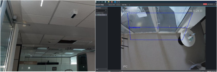
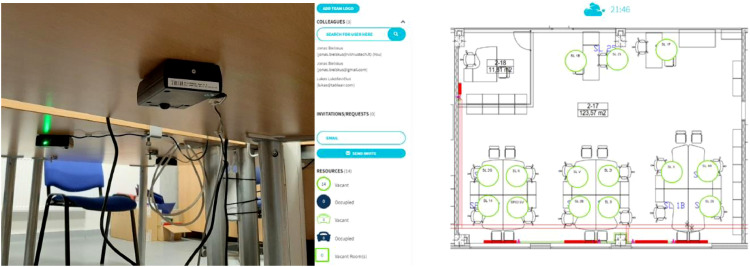
Measurement equipment characteristics are given in Table 2 . 3 D camera, used in Building A, is counting the number of persons entering and leaving the room and generates hourly reports. The camera is mounted at the entrance door (Fig. 3 ), and it is connected to a Wi-fi network enabling remote access. Alternatively, for desk occupancy measurement PIR + temperature sensors are used. The data of these sensors are considered as more precise as they are mounted under the desk (Fig. 4 ) and use double-check methodology – when occupants take a seat at the desk, PIR sensor reacts and temperature sensor additionally confirms the occupancy and just then signal is sent to the server. On the opposite, double-check is used when the occupant leaves the desk. The signals are also transferred remotely through Wi-fi for 1 min. time step. These sensors cannot monitor the overall occupancy of the room, compared to the 3D camera. In Building B, just desks occupancy is monitored.

Table 2.

Measurement equipment used for monitoring.

Equipment model	Measured parameter	Measurement limits	Accuracy	Time step
HOBO MX102A	CO2	0 – 5000 ppm	1 ppm	5 min
Hikvision ids-2cd6412fwd/c	Room occupants	Maximum 10 persons	Up to 98%	60 min
TABLEAIR SBL UNI SET	Desk occupancy	0 – +50 °C	0.5 °C	1 min

Table 3.

Weeks for weekly analysis.

Before quarantines (pre-pandemic)	2020, week No. 10
First quarantine	2020, week No. 16
Between the quarantines	2020, week No. 33
Strict second quarantine	2021, week No.7
Light second quarantine	2021, week No. 19
Post-quarantine	2021, week No. 28

Fig. 3.

Occupancy measurement with 3D camera.

Fig. 4.

Measurement of desks occupancy with PIR + temperature sensors.

The amount of data for one PIR + temperature sensor for building A is equal to 299 521 and for all 14 sensors, it results in 4 193 294 of data recorded with 1 min. time step. CO₂ concertation measurements were performed every 5 min. with 1 sensor in the room and resulted in 59 662 of data records. All the data gathered from Building A are processed and used further for actual occupancy schedules generation as well as for occupancy simulation with ELM-SA model.

For Building B, one PIR+temp sensor recorded up to 830 877 of data. Overall from 75 sensors recorded data every 1 min. constituted 62 315 775. These data were also processed and used for actual occupancy schedules generation.

2.2. Analysis of the actual occupancies

Actual occupancies are analysed for different periods of pandemic generating average hourly occupancies for one working day and analysing hourly occupancies on separate weekdays’ basis. In addition, occupancy frequencies, expressed in persons/m² for different periods are compared for both buildings. Comparison between buildings is possible just for 3 periods, where measurement time overlaps (Fig. 2). For Building B analysis of the 6 pandemic periods is informative, as it shows occupancy fluctuations before the pandemic and through the whole pandemic.

2.3. Prediction of the occupancy with ELM-SA model

Hypothesis, that prediction reliability may be influenced by a drastic decrease of the occupancy of the building during pandemics, is checked on Building A, as it has long-term measurement both for occupancy and for CO₂. CO₂ is considered the most suitable indoor parameter for occupancy prediction (Bielskus et al., 2020; Motuzienė et al., 2021). All the data gathered for this building are processed dividing them into 5 min. intervals. Afterwards they are imported into the ELM-SA model into Matlab software. The mathematical methods and models are described below. As both methods – ELM and SA are widely used and known, just principle description with created mathematical pseudocodes is given. The pseudocode of the ELM-SA is employed from Loopez-Fandino, Quesada-Barriuso, Heras and Arguello (2015); Ruiz-Torrubiano et al. (2010).

2.3.1. Extreme learning machine

ELM is a learning algorithm linked with Artificial Neural Networks (ANNs) and it was first introduced by Huang, Zhu and Siew (2004). Due to its extremely short calculation time and simplicity ELM is applied in various fields, such as medicine, marine, etc. (Chen, Song, Liu, Yang & Li, 2020; Storn et al., 1995, etc.). Different improvements of the algorithm have been proposed, thus enabling its applications also for big data analysis Chen, Li, Duan and Li (2017). Hence, the potential of the ELM until now is not sufficiently exploited in the field of the building's occupancy prediction, where both prediction accuracy and speed of the prediction is important as it is related to the control of the building services systems (Motuzienė et al., 2021).

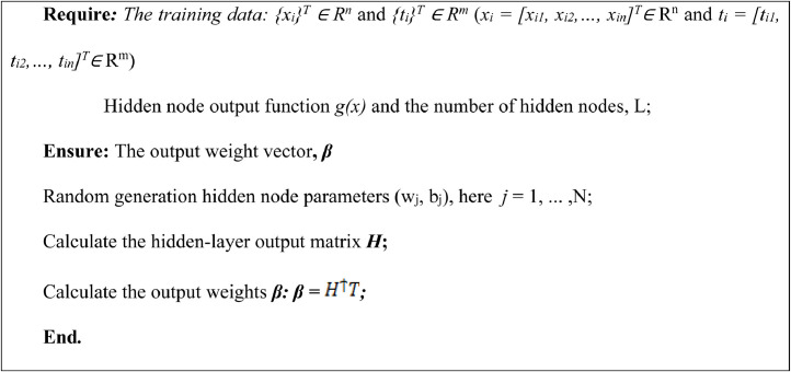
Single-layer Feedforward Networks (SLFNNs) architecture is constructed for N – arbitrary distinct samples (where x_i – CO₂ concentration and t_i – occupancy) with hidden nodes L and activation function g(x). The activation function is sigmoidal and it is infinitely differentiated. SLFNN is made up of three layers: input neurons, hidden neurons, and output neurons. For a set number of L hidden nodes input (w) and bias weights (b) are randomly generated and the output weight (β) matrix (H) is solved by minimizing the approximation error in the squared error sense and the smallest norm least-squares solution is reached by the Moore-Penrose generalization of the inverse matrix β =H†T . ELM standard pseudocode is given in Fig. 5 .

Fig. 5.

Pseudocode for the ELM algorithm.

Mostly common proportions of the data used in neural networks models for training, testing, and validation accordingly are 60/20/20% or 50/25/25% (Chen et al., 2020), but in this study, we use 70/10/20% based on recommendations given by )(Nguyen et al., 2021).

Assumptions for the simulations with SA-ELM model:

• •Number of hidden neurons – 25;
• •Maximums number of iterations (MaxIter) – 100.

Require:The training data: {xi}T ∈ Rn and {ti}T ∈ Rm (xi = [xi1, xi2,…, xin]T∈ Rn and ti = [ti1, ti2,…, tin]T∈ Rm) Hidden node output function g(x) and the number of hidden nodes, L; Ensure: The output weight vector, β Random generation hidden node parameters (wj, bj), here j = 1, …,N; Calculate the hidden-layer output matrix H; Calculate the output weights β: β =H†T ; End.

2.3.2. Simulated annealing optimisation algorithm

Simulated Annealing (SA) is a metaheuristic method, which was first presented by Kirkpatrick, Gelatt and Vecchi (1983) and is applied when solving different optimization problems Roshani, Salehi and Esfandyari (2013). It is based on the search of the global minimum of the specific objective function attempting to avoid local minimums by performing the random search (movements in the searched neighbourhood).

Before starting the SA - initial temperature (t₀), which is the main control parameter and is reduced during the optimisation process, must be set (Sieniutycz et al., 2018). Annealing starts when an initial solution (x₀) is generated and it is considered as the best present solution. Afterwards the neighbourhood structure is created - two positions i and j are selected and reverse, insert, and swap operators (N) are used to produce neighbouring solutions. The list of input data is created and the probability p of a candidate's decision is calculated. If the decision function f(x) is worse than the candidate decision function ((f(y)> f(x)), then the probability of acceptance is calculated. In each iteration, the maximum data are used from the list. Each time a bad candidate solution is met, a random number r is generated. If r < p, then the bad candidate solution will be accepted (Zhan, Lin, Zhang & Zhong, 2016). To update the data list the average of all data t_av is used. The optimisation stops when the lowest limit of the temperature is reached or a predefined number of iterations is reached.

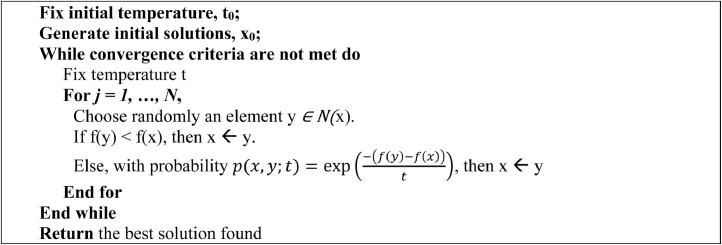
SA algorithm pseudocode is given in Fig. 6 .

Fix initial temperature, t0; Generate initial solutions, x0; While convergence criteria are not met do Fix temperature t For j = 1, …, N, Choose randomly an element y ∈ N(x). If f(y) < f(x), then x ← y. Else, with probability $p\left(x,y;t\right)=\text{exp}\left(\frac{-\left(f\left(y\right)-f\left(x\right)\right)}{t}\right)$, then x ← y End for End while Return the best solution found

Fig. 6.

Pseudocode for the SA algorithm (Ruiz-Torrubiano et al., 2010).

Occupancy prediction simulations are performed for the whole measurement period and for 3 pandemic periods separately to compare ELM-SA model performance reliability in terms of Root Mean Square Error (RMSE) (Carbone et al., 1982) and R-square (R²).

3. Results

3.1. Average working day occupancy profiles

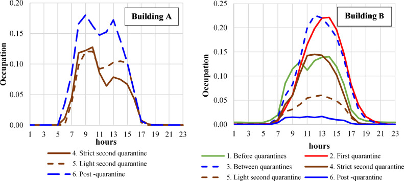
After processing measurement data, hourly occupancy profiles for the typical working day for both buildings were presented based on average values for separate the monitored periods (Fig. 7 ) (the same colours of lines in both graphs represent the same measured period).

Fig. 7.

Hourly working day actual average occupancy schedules for building A and building B based on PIR sensors measurements.

Building A. It is seen from the building A profiles, that actual occupancy during the strict quarantine and light quarantine was very similar and low – peaking on average at 0.12 (12% of the maximum possible occupancy) and even after the quarantine was cancelled it has raised, but not as significant as it was expected (just 0.2 – 20% of the maximum possible occupancy). This can be explained by two reasons: 1) summer period when part of the employees were on holidays and 2) changes in the working culture – switching more to the remote work.

Building B. A much longer monitoring period for Building B shows that average peak occupancy during the working day does not exceed 0.23, showing a low office area utilisation rate. It is also interesting that during the first quarantine office was occupied even more than before the pandemic, but this can be explained by the fact that the company was expanding at that time and people still worked in offices applying different safety strategies, e.g. leaving every second desk empty. And the maximum daily occupancies for the “light quarantine” and “post-quarantine” periods show tendencies to decrease to 0.06 and 0.02 accordingly and this may have similar explanations as for Building A. This office also has specifics – occupation duration (in hours) is much longer than for office A. In general, this office data does not reflect some specific influence of the pandemic on the occupancy.

Comparing for this building all of the periods' occupancies with standard ones proposed by ASHRAE 90.1 (peak occupancy fraction 0.9) or EN 16,798–1 (maximum occupancy fraction 0.7), occupancies are much lower than measured values. Therefore, this causes a certain energy performance gap related to occupants when comparing calculated and actual energy consumption as real occupancy has not much in common with the theoretical standard values.

3.2. Occupancy profiles analysis on separate weekdays’ basis

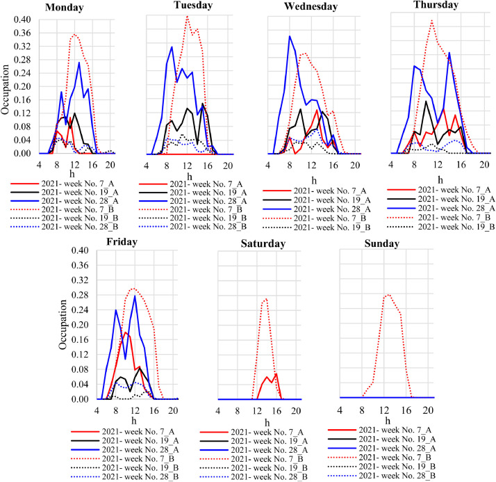
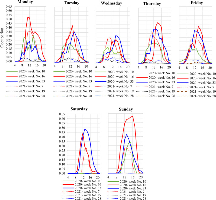
As average daily profiles do not always give the full view of the real situation if there are high fluctuations in occupancies within the week, a more detailed analysis was performed for each working day of the week (Fig. 8 ). To compare fluctuations of the occupancies within the week during the different pandemic periods, one week for each period was taken and presented (Table 3). Fig. 8 presents occupancies for both buildings and Fig. 9 presents occupancy just for building B with additional measurement periods, also the period before the pandemic started.

Fig. 8.

Hourly occupancy schedules for separate working days for the Building A and B.

Fig. 9.

Hourly occupancy schedules for separate working days for the building B.

Analysing actual occupancy schedules for separate measured pandemic periods day-by-day for Building A it can be noticed that for post-quarantine periods (Fig. 8) peak occupancy fraction reaches 0.34 on Wednesday and this is more than the average peak value of 0.23 discussed above. This period shows an obvious occupancy increase compared to both quarantine periods, but it is still low compared to the maximum possible. The occupancy, compared to the periods of quarantines, starts earlier in the morning – from 6:00 a.m. and ends between 3:00–5:00 p.m.

In contrast to Building A, for Building B occupancies were higher for the strict lockdown period peaking at 0.4 and being around 0.3 even during the weekend. Accordingly, the contrast is also noticed during the light quarantine and post-quarantine periods, when occupancies were extremely low (Fig. 8).

In Building B day-by-day data analysis revealed occupancy schedules different to typically found in literature or practise offices’ working schedules (Fig. 9). This building data enables us to compare fluctuations during the pre-pandemic period (2020 week No. 10). Same as discussed above (Fig. 7), the obvious relation of occupancy fluctuations to the pandemic cannot be noticed for this office. Occupation reaches maximum values within the first quarantine and surprisingly highest daily peak is on Sunday - 0.62. Before the pandemic highest peak was just 0.29 (the reasons for that were explained).

It is obvious that Building B is a very atypical office and its occupancy varies chaotically regardless of whether there is a quarantine in the country or not. For this reason, this building, other similar ones, where occupancy is difficult to predict, and constantly fluctuating, cannot be subject to building services systems management according to pre-set schedules, as this is simply energy inefficient and may not meet occupants' needs. Here occupancy prediction models and their integration into BMS (Building Management systems) are recommended to operate systems sustainably, based on real demand.

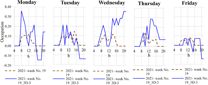
Measurements with 3D camera.Fig. 8-9 present results based on desks occupancy measurements with PIR+temperature sensors, but in Building A also 3D camera was used to measure the number of employees entering and leaving the office. The principle of how occupancy is calculated according to camera is based on Eq. (1):

$$O_t=O_{t-1}+O_{ten}+O_{tex},$$ (1)

where: $O_t$ – number of occupants at time t, $O_{t-1}$ – occupants present in the room before time t, $O_{ten},O_{tex}$ - number of occupants entering and exiting the room at time t. At midnight, the camera recordings are deleted and the new day starts with 0 occupancies. Occupancies measured with the 3D camera and PIR sensors were compared on an hourly basis for one week of “light second quarantine”. As it is seen from Figure 10, there is almost no correlation with the results of the PIR sensors, which use double-check methodology. Also, 3D cameras show negative occupancies or high occupancies late in the evening, when the room was empty. Therefore, in the authors' opinion, occupancy measurement with a 3D camera in a monitored office failed as measured values do not correspond to ground truth data. There may be different problems influencing the accuracy, e.g. occupant is counted 2 times (Hakan Cetinkaya & Muammer Ackay, 2015), with less than 6 people in a view camera may overestimate occupancy due to the shadows and non-human objects (Zhang, Venetianer & Lipton, 2008), etc. Specific algorithms might be required to increase the accuracy of cameras and to correct erroneous count data (Sangoboye & Kjærgaard, 2016). As an application of such algorithms is out of the scope of the study, just PIR+temperature sensors with double check methodology data are further considered as reliable.

Fig. 10.

Occupancy of building A measured with PIR sensors and 3D camera.

3.3. Occupancy densities analysis

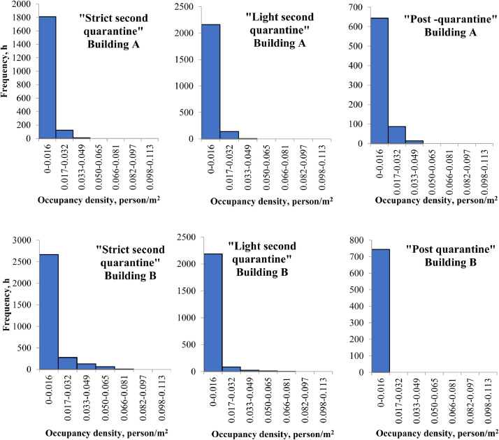
Some less sophisticated buildings' energy efficiency calculation methodologies or tools require to enter into the model as input just one number – occupant per area instead of hourly schedules. Therefore, histograms were produced to present what densities are common for the analysed buildings (Fig. 11). These values are easy to convert into the number of persons as they just need to be multiplied by the area of the room. Considering all the measurement periods for Building A occupancy density never reached more than 0.049 persons/m² and 92% of the time it did not exceed 0.016 persons/m². For Building B occupancies reached 0.113 persons/m², but occupancy between 0.066–0.113 was recorded just 1.5% of the time during 1 year and 8 months measurement period and 83% of the time it did not exceed 0.016 persons/m². Fig. 11 shows the occupancy densities comparison for both buildings. For both buildings dominant within all 3 pandemic period's occupancy density is up to 0.016 persons/m². And obviously, taking into account previously discussed results, for Building A it has slightly increased during the post-quarantine period, and for Building B it shows opposite tendencies.

Fig. 11.

Occupancy density frequencies for separate pandemic periods.

Measurements show low occupancy densities even for non-quarantine periods. For comparison, default density used in DesignBuilder simulation software for open-office buildings – 0.11 persons/m², in Lithuanian standard for Buildings energy performance assessment (STR, 2.01.02:2016) proposes one common value for all types of offices – 0.05 persons/m² average for the whole building area, so it would be even more for one office room. So results of the study indicate that the density of persons in offices is strongly overestimated and it has a tendency to decrease in the future. Low occupancies were also noted by the authors in their previous study, performed before the pandemic (Bielskus et al., 2020).

3.4. Occupancy prediction with ELM-SE model

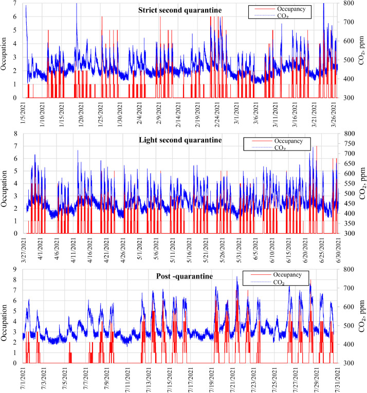
Fig. 12 presents actual measured CO₂ concentrations and occupancy with PIR+temperature sensors in Building A. it is obvious that CO₂ correlates with the occupancy (as people are the main sources of CO₂ in the room) and it was previously proven, that this parameter fits the best for the occupancy prediction with ELM models (Bielskus et al., 2020). It can be noted that maximum occupancy within the measured period is 8 persons and maximum CO₂ concentration – about 1100 ppm. Mostly maximum CO₂ concentration in the room is around 600–700 ppm and this is even less than required for IDA 1 indoor air category (limit 800 ppm). The room is over-ventilated and is not controlled according to demand thus wasting energy. Here BMS system with an occupancy prediction model would enable energy savings for ventilation.

Fig. 12.

Measured CO₂ concentration and occupancies for the building A for different pandemic periods.

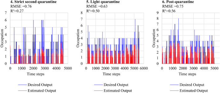
Occupancy prediction is performed for different periods of pandemic (Fig. 13) and the whole measurement period (Fig. 14). All the periods include data from more than 2 months. As it was concluded in previous studies (Bielskus et al., 2020; Motuzienė et al., 2021), a sufficient measurement period is 4 weeks. Here periods are much longer, but prediction accuracy is low (R²=0.27) for the period of strict quarantine and increases for light quarantine and post-quarantine accordingly up to R²=0.50; 0.56. That prediction accuracy of the model is low, compared to the once defined for the same model at pre-pandemic conditions, and the hypothesis, that ELM-SA model prediction reliability at pandemic conditions drops – is confirmed. It can be noticed, that predictability is lower at the periods when occupancy is very low (see also Fig. 7 for actual occupancies).

Fig. 13.

Occupancy prediction for different pandemic periods.

Fig. 14.

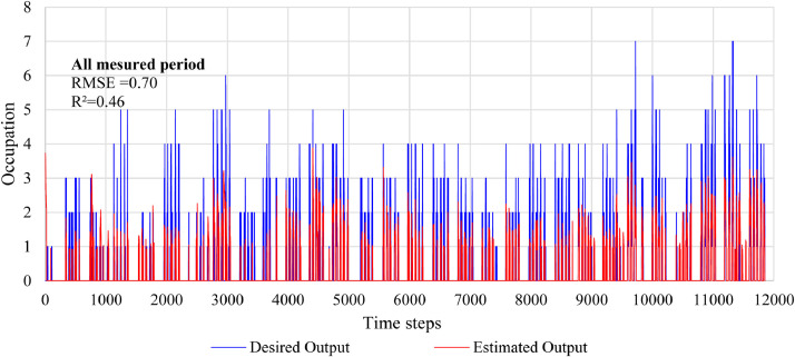
Occupancy prediction base on whole measured period data.

Fig. 14 also confirms that problem is not an amount of data, as even simulating with measurement data from all 8 months prediction reliability is even lower (R²=0.46; RMSE=0.70) than for “light quarantine” and “post-quarantine” periods. Again, confirms that the problem is low occupancy, which is related to low CO₂ values and if air mixing in the rooms is not ideal (and usually this is the case), the sensor does not record any changes in CO₂ concentration.

4. DISCUSSION

Office building‘s occupancy was always difficult to predict if an office has no strictly established working hours (e.g. as banks or governmental institutions). But during different pandemic periods related to quarantines, it fluctuates, but not as much as expected, and stays low even after quarantine. Analysis proves that the actual office area utilization rate depends on industry specifics and one common occupancy cannot be assumed during the design stage, it must be differentiated when possible. In the analysed buildings Building A is a professional services building and Building B is a manufacturing building. Building B has higher peak occupancies and they are not even dependant on pandemic conditions, this building has much longer occupancy hours and is occupied even during weekends (Fig. 7 and 10 ). Also for both offices it was found that occupancy densities are very low (Fig. 11 ) for different pandemic periods thus showing tendencies that offices’ area utilisation rates are low and more sustainable office area utilisation solutions are required.

Occupancy of Building B is a very good example of the office building, where occupancies are fluctuating without any clear tendencies (chaotically) and therefore such buildings cannot be sustainably controlled if pre-defined schedules are used in the Building management system (BMS). Such buildings required predictive dynamic control and here such models as ELM-SA have the potential to be integrated to increase the sustainable operation of the building. Building A is also obviously over-ventilated (Fig. 12 ), showing that the ventilation system does not react to actual occupancies and here demand-controlled ventilation also has a high potential for energy savings.

The hypothesis, that ELM-SA model prediction reliability at pandemic conditions drops (compared to previously found R₂ = 0.74) – is confirmed, as even long measurement periods give low accuracies (Fig. 13 , 14 ) - R² = 0.27–0.56. It was noticed, that predictability is lower at the periods when occupancy is very low. This shows that occupancy prediction based on CO₂ concertation when occupancy is very low and air mixing in the room is not ideal is not very sufficient. The pandemic is the case when occupancy is low and potentially will stay lower in the future after the pandemic ends.

5. Conclusions

• 1Analysis of the actual occupancies for different pandemic periods shows, that occupancies are very low during all the periods: average peak occupancy for Building A for different pandemic periods fluctuates from 12 to 20% and for Building B – from 2 to 23%. Occupants’ density for all the measurement periods for Building A never reached more than 0.049 persons/m² and 92% of the time it did not exceed 0.016 persons/m². For Building B - occupancies never exceeded 0.113 persons/m², but occupancies between 0.066–0.113 persons/m² were recorded just 1.5% of the time during 1 year and 8 months measurement period, 83% of the time it did not exceed 0.016 persons/m². For both buildings dominant within all 3 pandemic period's occupancy density is up to 0.016 persons/m².
• 2Occupancies and their fluctuations depend on the office industry. Building A representing professionals services office show occupancy decreases related to pandemic situation and manufacturing industry Building B – no tendencies at all and is occupied chaotically with different periods of pandemic and also within the weekdays.
• 3Both analysed buildings show the potential for energy savings if a predictive control system based on real demand, e.g. with an integrated ELM-SA occupancy prediction model, would be employed.
• 4ELM-SA occupancy prediction model reliability is influenced by pandemic conditions, as it showed dependency on occupancy – with low occupancies caused by pandemic its reliability has significantly dropped compared to normal (pre-pandemic) conditions and is found to be R² = 0.27–0.56 depending on a number of occupants.

Declaration of Competing Interest

The authors declare that they have no known competing financial interests or personal relationships that could have appeared to influence the work reported in this paper.

References

- Agarwal N., Swaroop C., Raj B.P., Saini L. Indoor air quality improvement in COVID-19 pandemic: Review. Sustainable Cities and Society. 2021;70 doi: 10.1016/j.scs.2021.102942. Article. [DOI] [PMC free article] [PubMed] [Google Scholar]
- Ai B., Fan Z., Gao R.X. Proceedings of the IEEE Conference—American Control Conference. ACC; Portland, OR: 2014. Occupancy estimation for smart buildings by an auto-regressive hidden Markov model—IEEE Conference Publication; pp. 2234–2239. 4–6 June 2014. [Google Scholar]
- Arup, (2021). Future of offices: In a post-pandemic world – Arup. Retrieved from https://www.arup.com/-/media/arup/files/publications/f/future-of-offices-in-a-post-pandemic-world.pdf.
- Azar E., Menassa C.C. A comprehensive analysis of the impact of occupancy parameters in energy simulation of office buildings. Energy and Buildings. 2012;55:841–853. doi: 10.1016/j.enbuild.2012.10.002. [DOI] [Google Scholar]
- Beaudoin, C., Georgules, J., & Raicht, T. (2020). Tenant needs in a post-pandemic world: 2020 Forecast series. Retrieved from https://www.us.jll.com/en/trends-and-insights/research/2020-first-look-navigating-post-COVID-19.
- Benita F. Human mobility behavior in COVID-19: A systematic literature review and bibliometric analysis. Sustainable Cities and Society. 2021;70 doi: 10.1016/j.scs.2021.102916. [DOI] [PMC free article] [PubMed] [Google Scholar]
- Bielskus J., Motuzienė V., Vilutienė T., Indriulionis A. Occupancy prediction using differential evolution online sequential extreme learning machine model. Energies. 2020;13(15):4033. doi: 10.3390/en13154033. [DOI] [Google Scholar]
- Carbone R., Armstrong J.S. Evaluation of extrapolative forecasting methods: Results of a survey of academicians and practitioners. Journal of Forecasting. 1982;1:215–217. doi: 10.1002/for.3980010207. [DOI] [Google Scholar]
- Cetinkaya H.H., Akcay M. People counting at campuses. Procedia-Social and Behavioral Sciences. 2015;182:732–736. doi: 10.1016/j.sbspro.2015.04.821. [DOI] [Google Scholar]
- Chen C., Li K., Duan M., Li K. Intelligent data-centric systems. Academic Press; Cambridge: 2017. Chapter 6 - Extreme learning machine and its applications in big data processing; pp. 117–150. [DOI] [Google Scholar]
- Chen Y., Song L., Liu ., Yang L., Li D. A review of the artificial neural network models for water quality prediction. Applied Sciences. 2020;10(17):5776. doi: 10.3390/app10175776. [DOI] [Google Scholar]
- Chen Z.H., Xu J.M., Soh Y.C. Modeling regular occupancy in commercial buildings using stochastic models. Energy & Buildings. 2015;103:216–223. doi: 10.1016/j.enbuild.2015.06.009. [DOI] [Google Scholar]
- Delzendeh E., Wu S., Lee A., Zhou Y. The impact of occupants’ behaviours on building energy analysis: A research review. Renewable and Sustainable Energy Reviews. 2017;80:1061–1071. doi: 10.1016/j.rser.2017.05.264. [DOI] [Google Scholar]
- Dong B., Andrews B., Lam K.P., Höynck M., Zhang R., Chiou Y.S., et al. An information technology enabled sustainability test-bed (ITEST) for occupancy detection through an environmental sensing network. Energy and Buildings. 2010;42(7):1038–1046. doi: 10.1016/j.enbuild.2010.01.016. [DOI] [Google Scholar]
- Dong B., Lam K.P. Building energy and comfort management through occupant behaviour pattern detection based on a large-scale environmental sensor network. Journal of Building Performance Simulation. 2011;4:359–369. doi: 10.1080/19401493.2011.577810. [DOI] [Google Scholar]
- Franco A., Leccese F. Measurement of CO2 concentration for occupancy estimation in educational buildings with energy efficiency purposes. Journal of Building Engineering. 2020;32 doi: 10.1016/j.jobe.2020.101714. [DOI] [Google Scholar]
- Geraldi M.S., Bavaresco M.V., Triana M.A., Melo A.P., Lamberts R. Addressing the impact of COVID-19 lockdown on energy use in municipal buildings : A case study in Florianopolis, Brasil. Sustainable Cities and Society. 2021;69 doi: 10.1016/j.scs.2021.102823. [DOI] [PMC free article] [PubMed] [Google Scholar]
- Guo M., Xu P., Xiao T., He R., Dai M., Miller S.L. Review and comparison of HVAC operation guidelines in different countries during the COVID-19 pandemic. Building and Environment. 2021;187 doi: 10.1016/j.buildenv.2020.107368. [DOI] [PMC free article] [PubMed] [Google Scholar]
- Han Z.Y., Gao R.X., Fan Z.Y. Proceedings of the 29th Annual IEEE International Instrumentation and Measurement Technology Conference (I2MTC), Graz, Austria, 13–16 May 2012. IEEE; GrazAustria: 2012. Occupancy and indoor environment quality sensing for smart buildings; pp. 882–887. https:/Doi.org/10.1109/I2MTC.2012.6229557. [Google Scholar]
- Happle G., Fonseca J.A., Schlueter A. A review on occupant behavior in urban building energy models. Energy and Buildings. 2018;174:276–292. doi: 10.1016/j.enbuild.2018.06.030. [DOI] [Google Scholar]
- Huang G.-.B., Zhu Q.-.Y., Siew C.-.K. 2004 IEEE International Joint Conference on Neural Networks. 2004. 2004. Extreme learning machine: A new learning scheme of feedforward neural networks; pp. 1098–7576. [DOI] [Google Scholar]
- International Energy Agency (IEA) Global Energy Review 2020 (2020). The impacts of the Covid-19 crisis on global energy demand and CO2 emissions. Available online: https://iea.blob.core.windows.net/assets/7e802f6a-0b30-4714-abb1-46f21a7a9530/Global_Energy_Review_2020.pdf.
- Ivanko D., Ding Y., Nord N. Analysis of heat use profiles in Norwegian educational institutions in conditions of COVID-lockdown. Journal of Building Engineering. 2021;43 doi: 10.1016/j.jobe.2021.102576. [DOI] [Google Scholar]
- Jiang P., Fan Y.V., Klemeš J.J. Impacts of COVID-19 on energy demand and consumption: Challenges, lessons and emerging opportunities. Applied Energy. 2021;285 doi: 10.1016/j.apenergy.2021.116441. [DOI] [PMC free article] [PubMed] [Google Scholar]
- JLL. Occupancy planning trend report. Utilization. Online access (last accessed 05.09.(2021)).: https://www.jll.co.uk/content/dam/jll-com/documents/pdf/personalized-benchmarking/jll-global-2020-op-benchmarking-report-design-utilization.pdf.
- Kang H., An J., Kim H., Ji C., Hong T., Lee S. Changes in energy consumption according to building use type under COVID-19 pandemic in South Korea. Renewable and Sustainable Energy Reviews. 2021;148 doi: 10.1016/j.rser.2021.111294. [DOI] [PMC free article] [PubMed] [Google Scholar]
- Kirkpatrick S., Gelatt C.D., Vecchi J.M.P. Optimization by simulated annealing. Science (New York, N.Y.) 1983;4598:671–679. doi: 10.1126/science.220.4598.671. [DOI] [PubMed] [Google Scholar]
- Krarti M., Aldubyan M. Review analysis of COVID-19 impact on electricity demand for residential buildings.(2020) Renewable and Sustainable Energy Reviews. 2021;143 doi: 10.1016/j.rser.2021.110888. [DOI] [PMC free article] [PubMed] [Google Scholar]
- Lang, J. (2020). Tenant needs in a postpandemic world. Retrieved from https://www.abettercity.org/assets/images/ABCC%20JLL%20Deck%205.12.pdf.
- Loopez-Fandino J., Quesada-Barriuso P., Heras D.B., Arguello F. Efficient ELM-Based techniques for the classification of hyperspectral remote sensing images on commodity GPUs. IEEE Journal of Selected Topics in Applied Earth Observations and Remote Sensing. 2015;8(6):2884–2893. https://ieeexplore.ieee.org/document/1380068. [Google Scholar]
- Lord, C. (2021). Co-working is the future: How shared office spaces could transform the post-COVID workplace. Rerieved from: Https://globalnews.ca/news/7898991/coworking-post-covid-office-spaces-canada/.
- Masoso O.T., Grobler L.J. The dark side of occupants’ behaviour on building energy use. Energy and Buildings. 2010;42:173–177. https://doi.org/10.1016/j. enbuild.2009.08.009. [Google Scholar]
- Mastropietro P., Rodilla P., Batlle C. Emergency measures to protect energy consumers during the Covid-19 pandemic : A global review and critical analysis. Energy Research & Social Science. 2020;68 doi: 10.1016/j.erss.2020.101678. [DOI] [PMC free article] [PubMed] [Google Scholar]
- Menezes A.C., Cripps A., Bouchlaghem D., Buswell R. Predicted vs. actual energy performance of non-domestic buildings: Using post-occupancy evaluation data to reduce the performance gap. Applied Energy. 2012;97:355–364. doi: 10.1016/j.apenergy.2011.11.075. [DOI] [Google Scholar]
- Motuzienė V., Bielskus J., Lapinskienė V., Rynkun G. Office Building's Occupancy Prediction Using Extreme Learning Machine. Model with Different Optimization Algorithms. Environmental and Climate Technologies. 2021;25(1):525–536. doi: 10.2478/rtuect-2021-0038. [DOI] [Google Scholar]
- Nguyen Q.H., Ly H., Ho L.S., Al-Ansari N., Le H.V., Tran V.Q., et al. Influence of Data Splitting on Performance of Machine Learning Models in Prediction of Shear Strength of Soil. Hindawi . Mathematical Problems in Engineering. 2021;2021:15. doi: 10.1155/2021/4832864. Article ID 4832864pages, 2021. [DOI] [Google Scholar]
- Page J., Robinson D., Morel N., Scartezzini J.L. A generalised stochastic model for the simulation of occupant presence. Energy & Buildings. 2008;40:83–98. doi: 10.1016/j.enbuild.2007.01.018. [DOI] [Google Scholar]
- Pan Y., Du C., Fu Z., Fu M. Re-thinking of engineering operation solutions to HVAC systems under the emerging COVID-19 pandemic. Journal of Building Engineering. 2021;43 doi: 10.1016/j.jobe.2021.102889. [DOI] [Google Scholar]
- Paris Agreement Paris Agreement to the United Nations Framework Convention on Climate Change. 2015;12 16-1104). https://treaties.un.org/doc/Publication/MTDSG/Volume%20II/Chapter%20XXVII/XXVII-7-d.en.pdf. [Google Scholar]
- Perkins K.M., Munguia N., Ellenbecker M., Moure-eraso R., Velazquez L. COVID-19 pandemic lessons to facilitate future engagement in the global climate crisis. Journal of Cleaner Production. 2021;290 doi: 10.1016/j.jclepro.2020.125178. Article. [DOI] [PMC free article] [PubMed] [Google Scholar]
- Roshani A., Salehi M., Esfandyari A.A. simulated annealing algorithm for multi-manned assembly line balancing problem. Journal of Manufacturing Systems. 2013;32(1):238–247. doi: 10.1016/j.jmsy.2012.11.003. [DOI] [Google Scholar]
- Ruiz-Torrubiano R., Suarez A. Hybrid approaches and dimensionality reduction for portfolio selection with cardinality constrains. IEE Computational Intelligence Magazine. 2010;5(2):92–107. doi: 10.1109/MCI.2010.936308. [DOI] [Google Scholar]
- Salimi S., Hammad A. Optimizing energy consumption and occupants comfort in open-plan offices using local control based on occupancy dynamic data. Building and Environment. 2020;176 doi: 10.1016/j.buildenv.2020.106818. [DOI] [Google Scholar]
- Salimi S., Liu Z., Hammad A. Occupancy prediction model for open-plan offices using real-time location system and inhomogeneous Markov chain. Building and Environment. 2019;152:1–16. doi: 10.1016/j.buildenv.2019.01.052. [DOI] [Google Scholar]
- Sandels C., Widen J., Nordstrom L. Proceedings of the 2015 IEEE Power & Energy Society General Meetin. Denver; CO: 2015. Simulating occupancy in office buildings with non-homogeneous Markov chains for Demand Response analysis. [DOI] [Google Scholar]
- Sangoboye F.C., Kjærgaard M.B. Proceedings of the 3rd ACM International Conference on Systems for Energy-Efficient Built Environments. New York, NY, USA; 2016. PLCount: A probabilistic fusion algorithm for accurately estimating occupancy from 3D camera counts; pp. 147–156. [DOI] [Google Scholar]
- Schoen L. Guidance for building operations during the COVID-19 pandemic. ASHRAE Journal. 2020;62(5):72–74. [Google Scholar]
- Sieniutycz S., Jeżowski J. Energy optimization in process systems and fuel cells. 3rd Ed. 2018. Brief review of static optimization methods; pp. 1–41. [DOI] [Google Scholar]
- Stahl, A. (2021). The future of offices and workspaces, post-pandemic. Retrieved from https://www.forbes.com/sites/ashleystahl/2021/04/16/the-future-of-offices-and-workspaces-post-pandemic/?sh=416646926442.
- Storn R., Price K. Differential evolution—A simple and efficient adaptive scheme for global optimization over continuous spaces. International Computer Science Institute, Technical Report TR-95-012. 1995 http://www.icsi.berkeley.edu/ftp/global/pub/techreports/1995/tr-95-012.pdf [Google Scholar]
- STR 2.01.02:2016 “Energy Performance of Buildings: Design and Certification”, approved by the Minister of the Environment of the Republic of Lithuania on November 11, (2016). [Online]. [Accessed 01.02.2021]. Available: Https://e-seimas.lrs.lt/portal/legalActEditions/lt/TAD/15767120a80711e68987e8320e9a5185.
- Wang C., Yan D., Jiang Y. A novel approach for building occupancy simulation. Building Simulation. 2011;4:149–167. doi: 10.1007/s12273-011-0044-5. [DOI] [Google Scholar]
- Wang J., Huang J., Feng Z., Cao S., Haghighat F. Occupant-density-detection based energy efficient ventilation system: Prevention of infection transmission. Energy and Buildings. 2021;Volume 240 doi: 10.1016/j.enbuild.2021.110883. [DOI] [PMC free article] [PubMed] [Google Scholar]
- Wang W., Chen J., Hong T. Occupancy prediction through machine learning and data fusion of environmental sensing and Wi-Fi sensing in buildings. Automation in Construction. 2018;94:233–243. doi: 10.1016/j.autcon.2018.07.007. [DOI] [Google Scholar]
- Wang Z.X., Ding Y. An occupant-based energy consumption prediction model for office equipment. Energy & Buildings. 2015;109:12–22. doi: 10.1016/j.enbuild.2015.10.002. [DOI] [Google Scholar]
- Xie X., Qiuchen Lu Q., Herrera M., Yu Q., Parlikad A.K., Schooling J.M. Does historical data still count? Exploring the applicability of smart building applications in the post-pandemic period. Sustainable Cities and Society. 2021;69 doi: 10.1016/j.scs.2021.102804. [DOI] [PMC free article] [PubMed] [Google Scholar]
- Zhan S., Lin J., Zhang Z., Zhong Y. List-based simulated annealing algorithm for traveling salesman problem. Corporation Computational Intelligence and Neuroscience 2016. 2016 doi: 10.1155/2016/1712630. [DOI] [PMC free article] [PubMed] [Google Scholar]
- Zhang X., Pellegrino F., Shen J., Copertaro B., Huang P., Saini P.K., et al. A preliminary simulation study about the impact of COVID-19 crisis on energy demand of a building mix at a district in Sweden. Applied Energy. 2020;280 doi: 10.1016/j.apenergy.2020.115954. [DOI] [PMC free article] [PubMed] [Google Scholar]
- Zhang Z., Venetianer P.L., Lipton A.J. A robust human detection and tracking system using a human-model-based camera calibration. The Eighth International Workshop on Visual Surveillance - VS2008. 2008 https://hal.inria.fr/inria-00325644. [Google Scholar]