A nationwide indicator to smooth and normalize heterogeneous SARS-CoV-2 RNA data in wastewater

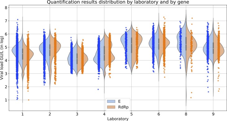
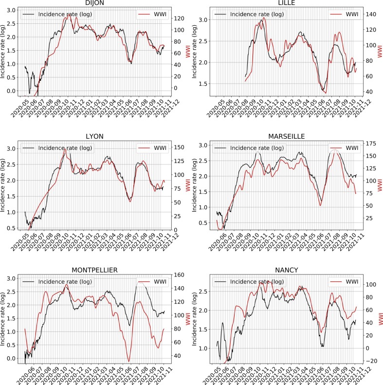
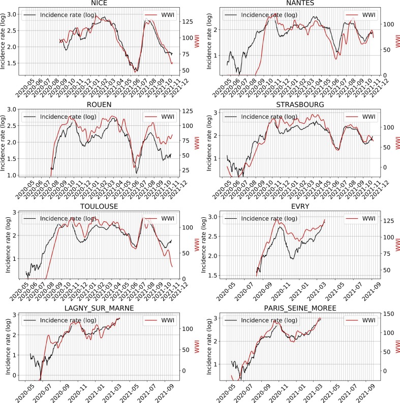
Graphical abstract

Abstract

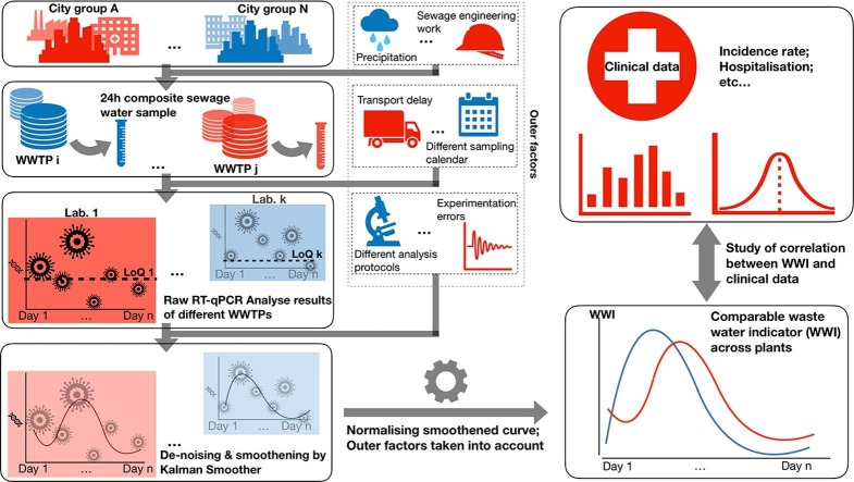
Since many infected people experience no or few symptoms, the SARS-CoV-2 epidemic is frequently monitored through massive virus testing of the population, an approach that may be biased and may be difficult to sustain in low-income countries. Since SARS-CoV-2 RNA can be detected in stool samples, quantifying SARS-CoV-2 genome by RT-qPCR in wastewater treatment plants (WWTPs) has been carried out as a complementary tool to monitor virus circulation among human populations. However, measuring SARS-CoV-2 viral load in WWTPs can be affected by many experimental and environmental factors. To circumvent these limits, we propose here a novel indicator, the wastewater indicator (WWI), that partly reduces and corrects the noise associated with the SARS-CoV-2 genome quantification in wastewater (average noise reduction of 19%). All data processing results in an average correlation gain of 18% with the incidence rate. The WWI can take into account the censorship linked to the limit of quantification (LOQ), allows the automatic detection of outliers to be integrated into the smoothing algorithm, estimates the average measurement error committed on the samples and proposes a solution for inter-laboratory normalization in the absence of inter-laboratory assays (ILA). This method has been successfully applied in the context of Obépine, a French national network that has been quantifying SARS-CoV-2 genome in a representative sample of French WWTPs since March 5th 2020. By August 26th, 2021, 168 WWTPs were monitored in the French metropolitan and overseas territories of France. We detail the process of elaboration of this indicator, show that it is strongly correlated to the incidence rate and that the optimal time lag between these two signals is only a few days, making our indicator an efficient complement to the incidence rate. This alternative approach may be especially important to evaluate SARS-CoV-2 dynamics in human populations when the testing rate is low.

1. Introduction

The SARS-CoV-2 pandemic has affected 214 million people worldwide and resulted in more than 6.6 million confirmed cases in France as of August 26, 2021. However, these figures underestimate the total number of infected people. Since massive individual testing may vary depending on the epidemiological situation and is economically difficult to sustain, particularly in low income countries, asymptomatic cases are hardly detected, except in a few scenarios of random tests, preparation for traveling, or contact cases (Gandhi et al., 2020, Mizumoto et al., 2020). Moreover, infected people with mild symptoms who do not seek medical assistance will not be screened either.

Several studies have demonstrated the value of wastewater-based epidemiology (WBE) for monitoring SARS-CoV-2 genome shedding in wastewater as a putative surrogate or complementary approach to classical epidemiological indicators (Wu et al., 2022, Wurtzer et al., 2020, Kocamemi et al., 2020, Hata et al., 2021, Anand et al., 2021). However, SARS-CoV-2 genome quantification in wastewater is subject to a number of shortcomings that must be corrected before such monitoring can be deployed on a large scale. These notably include (i) the intra-laboratory variability, i.e. the repeatability error on measurements from the same sample, (ii) the inter-laboratory variability, i.e. the difference in genomic units per liter of effluent evaluated by two different laboratories for identical samples even when using similar procedures; (iii) the specificity of each wastewater network (unitary or separative), its topography, the proportion of industries and the characterization of their discharges are also criteria of variability that must be taken into account to compare the evolution of the epidemics at a regional scale or to deduce the trend nationwide. The aforementioned variabilities must be corrected if the final purpose is a national monitoring network involving several laboratories, different protocols and many WWTPs. Several works have addressed the problem of mathematical processing of wastewater data. Some of them worked on the correlation between quantification results and new cases (Krivoňáková et al., 2021). Others have done extensive analysis on WBE uncertainty, including correction of quantification results with physico-chemical parameters, and have proposed solutions for automatic outlier detection (Wade et al., 2022). Others sought a way to communicate results to the general public with a more interpretable indicator than concentration values, by estimating the effective reproductive number, Re, from wastewater data (Huisman et al., 2021). However, to our knowledge, censoring of data below the LOQ has not been addressed in these studies. Outlier detection required additional modeling work and was not an integral part of the smoothing algorithm (Wade et al., 2022). Moreover, the selected smoothing solutions did not allow to estimate the average error of the measurement chain on the analyzed samples. Finally, the problem of standardizing results from different laboratories in the absence of inter-laboratory assays (ILA) was not addressed. We propose herein an original design of a uniform indicator, the wastewater indicator, that monitors the level of viral load in wastewater over time and accounts for the inherent variabilities in WBE. It can take into account the censorship linked to the LOQ, allows the automatic detection of outliers to be integrated into the smoothing algorithm, estimates the average measurement error committed on the samples and proposes a solution for inter-laboratory normalization in the absence of ILA. By August 26th 2021, 168 WWTPs were monitored twice a week by the Obépine network, a French national program that has been quantifying SARS-CoV-2 on some of the most important France’s WWTPs since March 3rd 2020. The performance of WWI was assessed on a subset of 24 WWTPs. The selection process of these WWTPs is detailed in Section 2.1. The robustness of this indicator to flow variations linked to various phenomena (rainfalls, civil engineering works on the network imposing the detour of the watershed towards other plants, etc.) was estimated. Then, the WWI was compared to local incidence rates on different Etablissements Publics de Coopération Intercommunale (EPCIs), French administrative structures regrouping several municipalities. This led us to estimate the correlation and the time lag between the WWI and the incidence rate, as well as the capacity of the WWI to anticipate major epidemiological changes (increased viral circulation, reduced circulation in response to governmental measures for example). This study focused on the peak of the so-called second wave that occurred in France during the fall of 2020.

2. Materials and methods

2.1. Data analysis

Statistical analyses were performed using R and Python programming languages. When not directly provided, the incidence and the screening rates were computed according to the formulas used by Santé Publique France (the French national public health agency), using a weekly moving average:

$$\begin{array}{c}{I}_r=100,000\times \frac{P}{\mathit{Pop}}\hfill \\ S_r=100,000\times \frac{T}{\mathit{Pop}}\hfill \end{array}$$ (1)

where $I_r$ is the incidence rate, $S_r$ is the screening rate, P is the number of people tested positive, T is the number of people tested, Pop is the sample population. Clinical data were then processed through additional smoothing of the Python statsmodels module to compensate for irregularities due to public holidays. All data of the 168 WWTPs were used to estimate the noise reduction provided by the method, by comparing the standard deviations of the signals before and after data processing. 24 WWTPs were considered for the remaining data analyses, with varying sampling frequency detailed later on. 22 WWTPs were selected for testing the impact of flow variations.

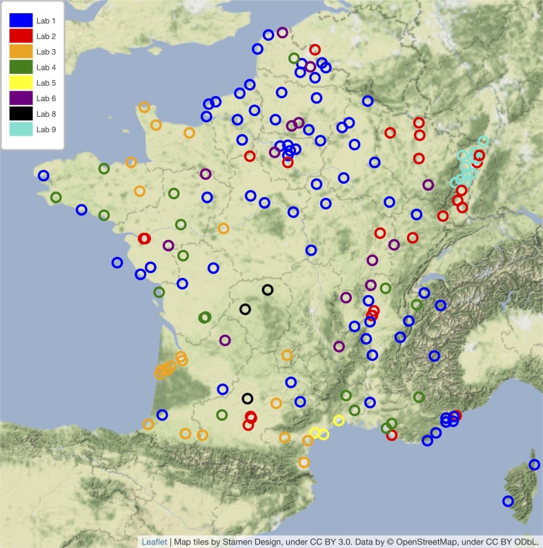
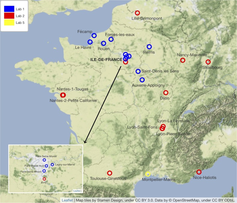
The selection criteria were established according to the following rationale. Among the 168 WWTPs monitored at the time of the analysis, we kept those which had at least 3 months of complete history, i.e. a minimum sample size. This sample size was therefore considered sufficient under the constraints of a test power of 80%, a significance level of 5%, as well as under the assumption of an effect size of 0.3 (Cohen’s d), corresponding to a small to medium effect size. Among the remaining WWTPs, we removed those which had known at least one week of vacancy (for technical reasons or end of the follow-up). We then considered all those which had at most 10% of flow values absent at the time of the analysis, hence the 22 WWTPs finally returned. Two additional WWTPs were considered for the statistical studies on correlation and time lag (Montpellier-Maera and Paris Seine-Morée), bringing the total number of WWTPs analyzed in the statistical studies to 24. The geographic distribution of the above 168 and 24 WWTPs is shown in Fig. 1 and Fig. 2 .

Fig. 1.

Map of the 168 WWTPs included in the Obépine monitoring network together with the corresponding laboratories responsible for the analyses.

Fig. 2.

Map of the 24 WWTPs involved in the statistical analyses.

The selection criteria for the correlation study were as follows. First, we selected the WWTPs and periods (second epidemic wave) where data were available from Santé Publique France at the watershed scale or the EPCI scale. That left 14 WWTPs for further selection. Additionally, we removed the WWTPs that covered only a fraction of the EPCI population. The 7 WWTPs resulting from this filtering were used to estimate the correlation gain with the incidence rate provided by the method. In order to estimate this correlation gain, we compared the correlation between the raw PCR quantification results and the incidence rate, with the correlation between the projections of these points on the WWI with the incidence rate. In order to estimate the noise reduction provided by the mathematical treatments, for each of the 168 WWTPs, we compared the standard deviation of the raw PCR quantification results to the standard deviation of the projection of these points on the WWI.

2.2. Sampling, transport and analysis

The statistical analyses in this document were performed on a portion of the wastewater samples collected between March 3rd 2020 and May 1st 2021. The protocol is as the following: wastewater samples were taken integratedly during a 24-h period, were conserved at 5°C (+/- 3°C) and transported at 4°C. Sampling protocols may slightly vary from WWTP to WWTP, but they all respect the French standard which asks for a volume-driven sampling rate; with subsamples of at least 50 mL, and at least 144 samples per day (one sample every 10 min on average). Quantification analyses, involving extraction, concentration and RT-qPCR or RT-dPCR steps (Wurtzer et al., 2020, Bertrand et al., 2021), were performed within 3 days from sampling. The data associated with these samples included incoming volume at the plant inlet, ammonium concentration, conductivity and chemical oxygen demand (COD). The results of the quantification (in number of genome unit per liter) and other related data were then processed by mathematical tools. RT-qPCR or RT-dPCR were performed on the E and RdRp genes, the former being routinely used to compute the WWI and the latter being used for validation purpose. Notably, RdRp quantification was used to confirm E quantification when outliers were detected on the E gene and as a motive to double check those values by performing the quantification process a second time.

2.3. Consideration of flow fluctuations at the wastewater treatment plant inlet

The WWI can have different quality indexes, thereafter called experimental data quality and precision indicator (EDQPI), depending on the richness of the data provided. We first pre-process the raw concentration ($C_{0,t}$) to account for external hydrological fluctuations. When accessible, the volume of wastewater reaching the WWTP, $V_t$, including flow diversion at the WWTP inlet in case of overloading, was used to compute daily virus loads from measured RNA concentrations (EDQPI = 2). When the volume was not available, a reference average daily volume was used ($V_0$), as provided by the French Ministère de la Transition écologique et solidaire for 2017 data (EDQPI = 1). An additional flux correction factor is applied when data are available. This factor is a function of ammonium, COD and conductivity concentrations, normalized by their mean dry weather value (EDQPI = 3).

$$C_t={\left(C_{0,t}\right)}_1\times {\left(\frac{V_t}{V_0}\right)}_2\times {\left(\frac{{\mathit{Poll}}_0}{{\mathit{Poll}}_t}\right)}_3$$ (2)

In order to understand the importance of these additional data, we estimated by simulation the difference between the WWI with quality indexes equal to 1 and 2. To do so, we first calibrated a parameterized statistic model under the two different settings of EDQPI 1 and 2, i.e., without and with inlet volume measurement respectively, hence we got two WWI curves of corresponding EDQPI. Then, for each of the two statistic models, we simulated a group of 1000 trajectories from its parameters. We finally computed the root-mean-square (RMS) deviation between the WWI of EDQPI 2 and each curve of each group of simulated trajectories. With the two sets of RMS deviations, we performed a one-factor ANOVA test to assess the impact of absence of daily incoming volume measurement of a plant, with null hypothesis being no significant difference between the 2 groups. We conducted the study on 22 WWTPs, each with several samples taken on rainy days with several months of history. We ran the same simulation to compare EDQPI 2 and 3, this time on 2 WWTPs for lack of sufficient physico-chemical data on the remaining sewage plants.

2.4. De-noising and interpolation through Kalman smoothing

RT-qPCR quantification is subject to many uncertainties. Using only the estimated viral genome concentrations to monitor the pandemic can therefore be misleading, as a large variation in the measured concentration can be due either to a real variation in virus concentration, or to a quantification error. This error can be caused by different factors, during the concentration, extraction or RT-qPCR steps, as well as during the integrated sampling at WWTP. Thus, standard materials and laboratory practices have a strong influence on the RT-qPCR performance (Bivins et al., 2021). Moreover, the genetic materials contained in the stools may change during their stay in the sewer system and during the aforementioned analysis steps (Kantor et al., 2021). This is why the raw viral load data are post-processed through Kalman smoothing (Rauch et al., 1965, Mayne, 1966, Fraser and Potter, 1969), in order to provide an estimate of the real amount of viral genome and to evaluate the uncertainty on this estimate. In this method, the existence of a time dependency between the actual quantities is exploited (i.e. the actual virus quantity in the wastewater on a given day provides information about the quantity that will be observed on the following days, due to the outbreak dynamics), while the successive errors in virus concentration measurements are independent from each other.

The concentrations to be measured are sometimes below the LOQs. Consequently, we face a problem of censored data. In addition, samples are typically collected twice a week, resulting in missing data on the other days. Finally, outliers may bias the smoothing. A new one dimensional Kalman smoothing method (Courbariaux et al., 2021) has been developed to adapt to these particularities for the needs of Obépine. We applied the developed smoother on the logarithm of the measured quantities in order to take into account the exponential character of the growth observed during the epidemic period and the heteroscedasticity observed empirically on the residuals when the method is applied directly.

The mathematical writing of the underlying model is as follows:

$$\begin{array}{cc}{X}_t\hfill & =\eta X_{t-1}+\delta +\kappa {\epsilon }_{X,t}\hfill \\ O_t\hfill & \sim \mathcal{B}(p)\hfill \\ (Y_t^{\ast }|O_t=0)\hfill & =X_t+\tau {\epsilon }_{Y,t}\hfill \\ (Y_t^{\ast }|O_t=1)\hfill & \sim \mathcal{U}([a,b])\hfill \\ Y_t\hfill & =\max (Y_t^{\ast },\ell )\hfill \\ \widehat{X_t}\hfill & =\mathbb{E}(X_t|Y_{t\in \mathcal{T}})\hfill \\ \left(\begin{array}{c}\hfill {\epsilon }_{X,t}\hfill \\ \hfill {\epsilon }_{Y,t}\hfill \\ \hfill \hfill \end{array}\right)\hfill & {\displaystyle \stackrel{i.i.d}{\sim }}\mathcal{N}(0,I),\hfill \end{array}$$ (3)

where t is the time index (ranging from 1 to n days), $X_t\in \mathbb{R}$ is the logarithm of the real concentration in wastewater at time $t,X={(X_t)}_{t\in \{1,\dots ,n\}}$ is the vector of log-transformed real concentrations (to be recovered) and $Y_t\in \mathbb{R}$ is the logarithm transformation of the estimated concentration in wastewater measured by RT-qPCR at time $t,C_t$, defined in Eq. 2 ($Y_t=\log (C_t)$). $Y_t$ is generally only partially observed. We note $\mathcal{T}\subset \{1,\dots ,n\}$ the set of t at which $Y_t$ is observed. $Y={(Y_t)}_{t\in \mathcal{T}}$ is the vector of measurements. $Y^{\ast }$ is an accessory latent variable corresponding to a non-censored version of Y. I is the identity matrix. $\eta \in \mathbb{R},\delta \in \mathbb{R},\kappa \in {\mathbb{R}}^{+}$ and $\tau \in {\mathbb{R}}^{+}$ are parameters (to be estimated). $\ell$ is the threshold below which censorship applies. $O_t\in \{0,1\}$ is, for any $t\in \mathcal{T}$, the indicator variable of the event ”$Y_t^{\ast }$ is an outlier”. $O={(O_t)}_{t\in \mathcal{T}}$. $\mathcal{B}(p)$ stands for the Bernoulli distribution of parameter p and $\mathcal{U}([a,b])$ for the Uniform distribution on the interval $[a,b]$. p is a meta–parameter designating the a priori probability of being an outlier (we take $p=2\%$ here). a and b have to be chosen, they can for example correspond to quantiles (respectively very close to 0 and very close to 1) of the empirical marginal distribution of Y. The parameters $\eta \in \mathbb{R},\delta \in \mathbb{R},\kappa \in {\mathbb{R}}^{+}$ and $\tau \in {\mathbb{R}}^{+}$ of maximum likelihood are estimated by numerical optimization through Nelder-Mead (Nelder and Mead, 1965) as explained in (Courbariaux et al., 2021). At time n, the developed smoother gives the law of $X_t$ for $t\in \{1,\dots ,n\}$ knowing $Y={(Y_t)}_{t\in \mathcal{T}}$, as well as the probability for each $Y_t$ to be an outlier. We note the produced reconstruction $\widehat{X_t}=\mathbb{E}(X_t|Y_{t\in \mathcal{T}})$.

2.5. Consideration of inter-laboratory variability

Several laboratories are providing sewage water SARS-CoV-2 viral load analyses to Obépine, each of them being in charge of several WWTPs. These laboratories have been selected based on their ability to carry out analyses properly using protocols that have been validated for the quantification of SARS-CoV-2 in wastewater (Wurtzer et al., 2020, Bertrand et al., 2021). Nonetheless, comparative inter-laboratory assays (ILA) have demonstrated that the estimated virus concentrations obtained on the same samples by different laboratories could sometimes differ in the order of magnitude of 1 log, as shown in Table 1 , which provides detailed information on the quantification techniques and responsibilities of the different laboratories involved in the project. In order to obtain a universal indicator for normalizing data provided by different laboratories (Baldovin et al., 2021), the level of the indicator for a specific plant is related to the maximum concentration recorded by its associated laboratory on all the plants assigned to it within the Obépine network over a specific period. We have chosen a period between June 1st 2020 and January 1st 2021, which gives a maximum corresponding to the peak of the second wave of the epidemic. We then perform the following normalization:

$${\mathrm{WWI}}_t=150\frac{\widehat{X_t}-\log (C_m)}{\log (C_M)-\log (C_m)}$$ (4)

Where ${\mathrm{WWI}}_t$ is the WWI value at time $t,\widehat{X_t}$ is the previously defined reconstruction, $C_m$ represents a quantification threshold of 1000 GU/L and $C_M$ is the maximum concentration historically recorded by the reference laboratory on plants with average daily flows similar to that of the plant of interest. The normalization factor of 150 was chosen a posteriori, so as to obtain a level between 40 and 85 around the beginning of September 2020, a period which corresponds for the majority of the plants to the middle of the exponential growth phase of the second wave in France. The maximum concentration is not solely based on the laboratory’s history, but more specifically on the basis of plants with a similar flow to the one to be standardized. This additional stratification by inflow volume strengthens the comparability among agglomerations whose population size is different and where the epidemic situations are similar. Precisely, in a scenario where a healthcare center that receives most of the Covid-19 patients of a neighborhood is connected to a small sewage network, the wastewater going into the corresponding WWTP would have extremely high level of viral concentration that could be seen nowhere else. Should this level of viral concentration be used in our Min–Max normalization, all other plants analyzed by the same laboratory would be heavily underestimated. We then chose to split the sewage plants in ten bins, according to their average daily incoming volume, and assign a maximum concentration to each category.

Table 1.

May 2021 ILA results as scaling factors between the 9 Obépine laboratories, in relation to one laboratory taken as reference (Lab 1). The number of WWTPs monitored and the LOQs reported by the laboratories are also indicated. Lab 7’s responsibilities did not include operational analyses for the monitored WWTPs.

	Lab 1	Lab 2	Lab 3	Lab 4	Lab 5	Lab 6	Lab 7	Lab 8	Lab 9
Scaling factor mean	1	0.95	1.20	1.96	3.96	10.64	0.40	6.50	1.12
Scaling factor std	0	0.31	0.34	0.54	0.74	9.00	0.077	2.62	0.43
Number of WWTPs	73	25	21	18	3	14	0	3	11
Quantifying technique	qPCR	qPCR	qPCR	qPCR	dPCR	qPCR	qPCR	qPCR	qPCR
LOQ (GU/L)	${1.10}^3$	${5.10}^3$	${5.10}^3$	$1,{1.10}^3$	$5,{5.10}^2$	${4.10}^4$	${1.10}^3$	${5.10}^3$	${4.10}^4$

This formula still had a major drawback in the case of laboratories joining the project later than the historical ones, typically after December 2020. To deal with this flaw, once ILA were performed, we used their results to assess and update a proportionality coefficient between laboratories running the same protocol. For a laboratory joining late with no historical record, we multiply its analysis results by this proportionality coefficient and use the $C_M$ of the laboratory we have chosen as the reference for the calculation of this coefficient. Finally, under logistics and transport constraints and the workload limit of the laboratories, we designed that each laboratory receives and analyses sewage samples from plants distributed as evenly as possible over the French territory. This choice avoids the situation where one laboratory is assigned only to cities with a low incidence of the disease and another to cities with a high incidence of the disease, a situation that would make it difficult to compare the viral load results between laboratories. The consideration of this inter-laboratory variability allowed us to aggregate the WWI of different WWTPs and elaborate regional indicators to have a more objective insight of the epidemic situation on a larger scale. Each regional indicator represents the weighted average of the local indicators in the same area, with the weight of each plant corresponding to its average daily volume.

3. Results

The results of the different mathematical treatments presented in Section 2 to convert the estimated amount of viral genomes entering a WWTP per day into a unitless value are illustrated in this section. We propose a new indicator: the WWI, which provides a smooth trend curve that is shown to accurately reflect the epidemic situation of a WWTP.

3.1. De-noising and interpolation through Kalman smoothing

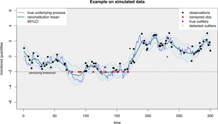
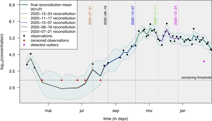
The results of this post-processing are illustrated on an example of simulated data (Fig. 3 ) and on a set of real data from the Obépine network (Fig. 4 ). As shown in Fig. 3, the mean signal reconstituted through this model faithfully reflects the true underlying process and shows low sensitivity to outliers. The successive reconstructions of the underlying ”true” auto-regressive process are expected to change at each new data point, since those bring additional information with regard to the past. This is depicted Fig. 4, with successive reconstructions proposed at different time points. Each intermediary reconstruction lies within the 95% prediction interval of the final reconstruction. The difference between the final reconstruction and each of the intermediary reconstructions is quite low, indicating that there are only minor differences between the results transmitted at a given date and those transmitted later on with additional data points.

Fig. 3.

An example of the application of the proposed smoother (taking into account censoring and outliers) on a set of simulated data including $16\%$ of censored data and $p=2\%$ of outliers. The censoring threshold corresponds to the RT-qPCR LOQ. The 95% prediction interval should cover about 95% of the true underlying process (blue curve). The mean reconstruction is faithful to the true underlying process. (For interpretation of the references to colour in this figure legend, the reader is referred to the web version of this article.)

Fig. 4.

An example of the application of the proposed smoother (taking into account censoring and outliers) on data from a wastewater treatment plant of the Obépine network: successive predictions for the underlying process (never observed), $X,95\%$ prediction interval and detected outliers (with an outlier proportion of $p=2\%$). The censoring threshold corresponds to the RT-qPCR LOQ. Each vertical dotted line corresponds to intermediary reconstructions over the course of the monitoring, without taking into account any additional data point beyond the reconstruction date. Only minor differences have been observed between these intermediary reconstructions and the final reconstruction. The WWTP is the one in charge of the EPCI of Dijon, and was associated with laboratory 2, see Table 1.

3.2. Impact of inflow variation on the WWI

Each trend curve is associated with a reliability index (EDQPI). EDQPI equals 1 when the WWI is calculated with an estimated flow and 2 when the real wastewater flow is used. By using the actual inflow volume of a plant, dilution effects by one-time events such as precipitation and civil engineering on the sewage network can be counterbalanced. This led us to estimate the impact of rainfall on local trend curves. Table 2 shows that the difference between WWI signals calculated with EDQPI 1 and EDQPI 2 data is statistically significant in 21 of 22 WWTPs. The only case for which the null hypothesis is not rejected is Rouen, which is one of the plants sampled only once a week. With an average of 180 rainy days per year, it is conceivable that the test result would be different with a higher sampling frequency. Therefore, this result indicates that plant inflows needs to be informed as soon as possible to improve EDQPI and primarily during periods of prolonged rainfall or reduced flow, regardless of plant size. We also tested the differences between quality indexes 2 and 3 at two plants. EDQPI is set to 3 when physico-chemical factors can be measured on samples such as ammonium concentration, conductivity and COD. The ANOVA results suggest that the difference is not significant (i.e., an EDQPI of 2 would be as effective in accounting for rainfall as an EDQPI of 3), although further investigation on a larger number and a wider variety of plants would be required.

Table 2.

Significance test results for difference between EDQPI 1 and EDQPI 2. %pop: % of the population of the urban unit connected to the WWTP; #P: Number of WWTPs that treat the main city; Cities: Number of cities connected to the WWTP; Ratio: ratio between the population of the main city over the sum of the populations connected to the WWTP; Lab: Index of the laboratory responsible for the analyses; Samples per week: number of samples collected per week, on average.

WWTP	Catchment population	%pop	#P	Cities	Ratio	Lab	Samples per week	p-value
Forges-les-eaux	16 000	100	1	3	0.73	1	1	<0.0001
Fécamp	45 000	100	1	4	0.85	1	1	<0.0001
Saint-Denis lès Sens	64 000	100	2	7	0.67	1	2	<0.0001
Auxerre-Appoigny	83 000	100	1	5	0.78	1	2	<0.0001
Nantes-2-Petite Californie	180 000	27	2	8	0.70	2	2	<0.0001
Evry	220 000	100	1	16	0.31	2	2	<0.0001
Lyon-La Feyssine	300 000	11	6	65	0.57	2	2	<0.0001
Le Havre	320 000	100	1	20	0.72	1	1	<0.0001
Lagny-sur-Marne	350 000	100	1	26	0.10	1	2	0.0017
Dijon	400 000	96	1	18	0.68	2	2	<0.0001
Lille Grimonpont	420 000	28	2	14	0.39	2	2	<0.0001
Reims	470 000	100	1	18	0.82	1	7	<0.0001
Nancy-Maxeville	500 000	100	1	23	0.38	2	2	<0.0001
Rouen	550 000	78	1	35	0.30	1	1	0.488
Paris Marne Aval	550 000	5	3	16	0.24	1	2	<0.0001
Nantes-1-Tougas	600 000	74	2	12	0.62	2	2	<0.0001
Nice-Haliotis	620 000	57	1	18	0.85	2	2	<0.0001
Lyon-Pierre Bénite	630 000	38	6	65	0.57	2	2	<0.0001
Toulouse-Ginestous	950 000	70	15	27	0.77	2	2	0.034
Lyon-Saint-Fons	980 000	47	6	65	0.57	2	2	<0.0001
Strasbourg	1 000 000	100	1	28	0.58	2	2	0.0012
Paris Seine Amont	3 600 000	33	3	125	0.24	1	2	<0.0001

3.3. Consideration of inter-laboratory variability

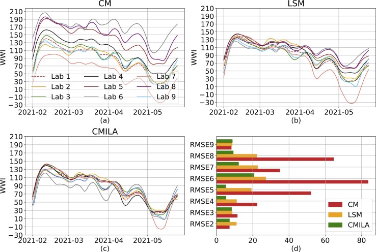
We take a critical look at the normalization technique we used to account for the inter-laboratory variability. As no WWTP has been analyzed by at least two different laboratories over the course of the project, we simulated an hypothetical behavior of a network with only one plant analyzed by the 9 Obépine laboratories. We chose one laboratory as a reference (Lab 1), and simulated quantification results varying from this reference, using May 2021 ILA results summarized in Table 1. To do so, we simulated a synthetic signal and assigned it to Lab 1. Then, using Table 1, we synthesized 8 others signals using scaling factors drawn from normal distributions whose parameters were estimated using May 2021 ILA results. For each sampling date and each laboratory, a credible scaling factor was drawn from these normal distributions. We compared three normalization techniques. CM refers to a single common maximum (CM) concentration among all laboratories. LSM refers to the modeling we used, with a laboratory-specific maximum (LSM) concentration. CMILA refers to a single common maximum concentration after scaling all the laboratories results to a reference laboratory using ILA results. Fig. 5 shows that our normalization technique significantly reduces the inter-laboratory variability for laboratories 4 to 8. Results are not significantly improved for the remaining 3 laboratories, as their scaling factors are close to 1 and their inter-samples replicability is quite good. Results can still be significantly improved, especially for lower values of WWI, once ILA are carried out.

Fig. 5.

Simulation of different inter-laboratory variabilities and normalization techniques. We simulate the simple case of a single plant analyzed by the 9 laboratories associated with Obépine. Panel (a) shows the results if the WWI normalization formula is applied with a $C_M$ common to all laboratories. Results show a clear disparity between laboratories and a strong attenuation towards laboratories with lower quantification results than laboratory 6. Panel (b) illustrates the correction brought by using a $C_M$ specific to each laboratory. Results are significantly improved for laboratories 4 to 8. The difference is not significant for the remaining 3 laboratories which all have a scaling factor close to 1 and a good inter-samples replicability. Panel (c) shows the correction brought by using ILA results and estimating a scaling factor between each laboratory and Lab 1. As shown in (d), CMILA still is the overall best normalization technique. CM, LSM and CMILA stands for a common maximum, a laboratory-specific maximum and a common maximum after scaling following ILA, respectively. Root mean square errors (RMSE) are calculated using the Lab 1 as reference.

3.4. Correlation and lag between the WWI and the incidence rate

In this section, we show how the WWI correlates with local incidence rate and how we find the time lag between the two signals using their correlation.

This study was done on 7 WWTPs of our network of 168 plants for reason of data availability. There are 22 EPCIs whose local incidence rate is an open data. We selected among these EPCIs whose sewage network connects to one single WWTP, so that the WWTP of the EPCI gathers as complete virological information as possible, minimizing the risk of not capturing an outbreak in some cities within the EPCI whose sewage networks connect to other WWTPs. The complete extension of the sewage network connected to a WWTP is particularly important in the study of correlation between the WWI and the local incidence rate, because any lack of information can lead to inaccurate estimation of correlation and the optimal lag between the WWI and the incidence rate. The chosen EPCIs are of varying size and are from different regions, the wastewater analyses results of these EPCIs come from three different laboratories.

Since the epidemic situation evolves rapidly, the testing behavior of an EPCI can change over time (due to factors like the test capacity, the population’s willingness of getting a test, the vaccination policy, etc), hence the incidence rate does not always reveals the same information of the population. Moreover, in France, individual test results are reported by city of residence and not by city where the test was performed. We chose the period from the 1st September 2020 to the nearest retake of the pandemic for this study. Reasons for the choice are, firstly it is a period when the holiday mode ends and most people return to a normal work regime, which means a more regular and limited population movement among neighboring cities, with our selection criteria mentioned above, this maximizes the overlapping between the populations sampled by the two signals; secondly, by that moment, the test capacity was adequate to test more than just symptomatic population and people were more likely to get tested in order to prepare for school and work, making the incidence rate more representative; thirdly, the chosen period contains both the blowing up and the cooling down phases of the second pandemic wave in France, this allows the study to focus on a rather complete life cycle of an outbreak.

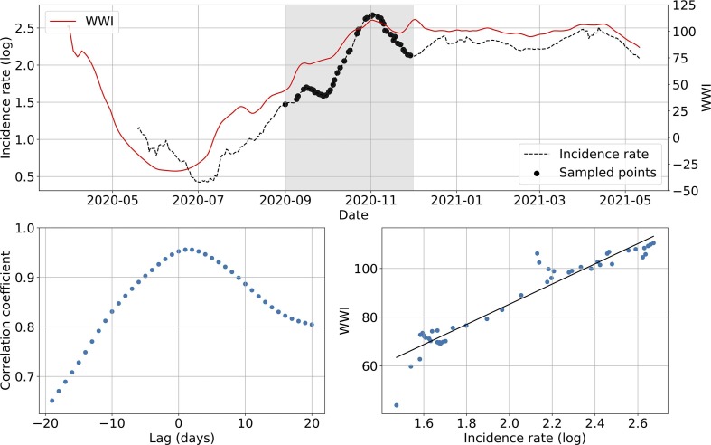
Cross-correlation, performed between the WWI and the log transformation of the incidence rate, was used as a measure of similarity between the two signals. To find the optimal lag between the two signals, we first take the logarithm of the incidence rate, then drag the subpart of the incidence rate curve over a +/- 20-day window until we find the time lag that maximizes the cross-correlation. Since correlation is sensitive to outliers especially when sample size is small, we subsampled the incidence signal using 50% of the available data so as to avoid certain special patterns resulting in an unnaturally high correlation. The time lag resulting the highest positive correlation is recorded. A positive lag value indicates that the WWI is ahead of the studied epidemic signal. A negative lag value indicates that the WWI is lagging behind it.

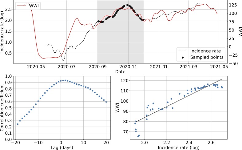
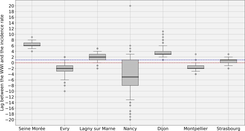
Fig. 6 shows an example of subsampling performed on the Lagny-sur-Marne WWTP. There is a strong correlation (> 0.92) between the WWI and the incidence rate during the second wave for this WWTP. Moreover, the optimal phase shift between the two signals is quite low (2 days), meaning the WWI was a great surrogate to the incidence rate at that time. Fig. 7 and Table 3 show some variance between WWTPs on the time lag and the correlation between WWI and incidence rate. Such a variance in time lag between WWTPs has already been reported (Fernandez-Cassi et al., 2021).

Fig. 6.

Subsampling example on the Lagny-sur-Marne WWTP. The top plot shows WWI and incidence rate curves as well as the sample points selected for that simulation (the shadowy area corresponds to the period of interest). The bottom left plot displays the computed correlation values for lag values varying between −20 and 20 days. A positive lag means that the WWI is ahead of the incidence rate. A negative lag means that the WWI is lagging behind the incidence rate. The bottom right plot displays a scatter plot of WWI vs incidence rate at best time lag (2 days, with a correlation coefficient of 0.93), as well as the linear regression fitted on the data.

Fig. 7.

WWI and incidence rate lag estimates, in days ($n=1000$ subsampling experiments with random sampling of 50% of incidence rate curve). A positive lag means that the WWI is ahead of the incidence rate. A negative lag means that the WWI is lagging behind the incidence rate. The Red dotted line indicates the zero offset level. The Blue dotted line is the median level over the 7 medians. The intra-experimental variance is significantly higher for the WWTP of Nancy, whose samples were not 24 h-integrated before October 20th 2020, leading to a more pronounced noise on the first half of the wave. (For interpretation of the references to colour in this figure legend, the reader is referred to the web version of this article.)

Table 3.

WWI and incidence rate lag estimates during the second wave in France (Fall 2020). Best correlation is the median of the best correlation over 1000 subsampling experiments. Montpellier was sampled once a week at that time. *Strasbourg, Nancy, Evry and Dijon were sampled once a week until mid October 2020, then twice a week. Lagny and Seine-Morée were sampled twice a week. Lab indicates the laboratory responsible for the analyses. A positive lag means that the WWI is ahead of the incidence rate. A negative lag means that the WWI is lagging behind the incidence rate.

	Nancy	Evry	Montpellier	Dijon	Lagny	Seine-Morée	Strasbourg
Lag (days)	−5	−2	−2	3	2	6	1
Lab	2	2	5	2	1	1	2
Sampling frequency (days)	2*	2*	1	2*	2	2	2*
Best correlation	0.76	0.86	0.88	0.89	0.92	0.94	0.95

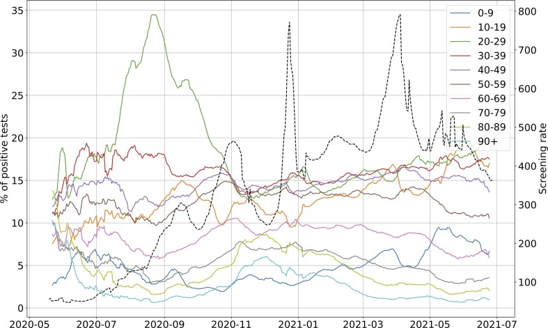
The intra-experimental variance is significantly higher for the WWTP of Nancy, whose average correlation with the incidence rate is not as strong as that of the other WWTPs. As the samples were grabbed and not integrated over 24 h until October 20th, 2020 for this plant, it cannot be excluded that the correlation is weaker due to a more pronounced noise on the samples taken before this date (Hata et al., 2021). As previously argued, we did not consider the time period between July and August 2020, one of the reasons is that we may have detected an earlier emergence of the pandemic than the incidence rate, as witnessed before by (Ahmed et al., 2021), but we cannot objectively prove it. For the early alert potentially detected by the WWI, an explanation could be that, by the time, it was mainly younger populations that were affected, among which less symptomatic cases were reported. It is then reasonable that the proportion of tested positive to total infected was rather low and thus conceivable that the WWI signal differs more significantly from the incidence rate during that period, because the two indicators monitored different populations by that time than at the second peak of the epidemic. Such a change in the demographic of the pandemic has already been reported in the state of Massachusetts (Xiao et al., 2021) and is illustrated in Fig. B.1.

Fig. B.1.

Evolution of the ratio of positive tests among each age bracket in France (solid lines) and of the screening rate (black dotted line). The screening rate corresponds to the number of test performed in France per 100,000 inhabitants. 20–29 years old bracket peaked during Summer 2020 and accounted for around 35% of the positive tests at its peak on August 21st 2020. Overall, the ratio increased from early June 2020 to late August 2020 among this age bracket. Conversely, the ratios among 40 years old and older categories were dwindling from July or even earlier for some of them. Infections were thus predominant among young people during Summer 2020 and less likely to be detected through conventional testing as the screening rate was about 3 times less important than at the peak of the second wave.

Overall, there is a good correlation between the two signals (>0.85 for every WWTP except Nancy), which is consistent with the results of (Wu et al., 2022, Wurtzer et al., 2020, Hata et al., 2021, D’Aoust et al., 2021, Medema et al., 2020, Ahmed et al., 2020, Peccia et al., 2020). There is an inter-WWTP variance in median time lag, as seen in Table 3, and it is going to be discussed in Section 3.5. As it stands, regional WWIs are still imperfect. They monitor a less evenly distributed population than regional incidence rates. Yet, they still show a good correlation (minimum correlation of 0.8) with their clinical counterparts, as shown in Fig. 8 and Table 4 . Moreover, the regional WWI peaks before regional hospitalizations for the two regions studied as examples in the second wave, which is consistent with the findings of (Saguti et al., 2021, D’Aoust et al., 2021). This illustrates the good aggregation capability of the WWI thanks to the normalization techniques we used, and our ability to follow the epidemic situation at a larger scale, despite monitoring at best less than 60% of a region’s inhabitants, as shown in Table 4.

Fig. 8.

Subsampling example for the Grand-Est region and the incidence rate. The top plot shows WWI and incidence rate curves as well as the sample points selected for that simulation (the shadowy area corresponds to the period of interest). The bottom left plot displays the computed correlation values for lag values varying between −20 and 20 days. A positive lag means that the WWI is ahead of the incidence rate. A negative lag means that the WWI is lagging behind the incidence rate. The bottom right plot displays a scatter plot of WWI vs incidence rate at best time lag (1 day, with a correlation coefficient of 0.96), as well as the linear regression fitted on the data.

Table 4.

Regional WWI correlation and lag estimates with incidence rate and hospitalizations during the second wave of Fall 2020. Best correlation is the median of the best correlation over 1000 subsampling experiments. IR means the WWI is compared with the incidence rate, H means the WWI is compared with the daily new hospitalizations in the corresponding region. The estimated surveyed population was calculated by considering the volume $V_{\mathit{db}}$ of each plant and a daily consumption of 200 L per inhabitant. A positive lag means that the WWI is ahead of the incidence rate. A negative lag means that the WWI is lagging behind the incidence rate.

	Iˇle-de-France - IR	Iˇle-de-France - H	Grand-Est - IR	Grand-Est - H
Lag (days)	-2	7	2	8
Number of laboratories	3	3	4	4
Number of WWTPs	7	7	28	28
Estimated surveyed population	33.1%	33.1%	58.6%	58.6%
Best correlation	0.81	0.86	0.94	0.97

3.5. Impact of the sampling frequency

The monitored WWTPs are collected twice a week, except for a few rare exceptions including the Reims WWTP, which is usually analyzed every day of the week. Since the Reims WWTP has been monitored for more than a year, it can be used to study the impact of the sampling frequency on the WWI signal. To do so, we compared its WWI signal computed from daily samples to potential WWIs obtained from different subsamplings of lower frequency. We varied the sampling frequency from one to six days per week. In our subsampling scenarios, we avoided consecutive sampling days as much as possible. In other words, we tried to spread the sampling days over a week as much as possible when choosing the combinations.

We then used two metrics to quantify this impact: RMSE between each WWI signal and cover rate between their respective 95% prediction intervals. We define the cover rate CR with the following formula:

$$\mathrm{CR}=\frac{2\times S_{\mathrm{common}}}{S_1+S_2}$$

where $S_{\mathrm{common}}$ is the intersection area between the two prediction intervals (see Fig. 10 ), $S_1$ and $S_2$ being the areas of the prediction intervals of the considered models. We chose this formula and not only the $S_{\mathrm{common}}$ to account for the case where wider prediction intervals, implying greater uncertainties, would lead to greater cover rates than better models with narrower intervals because they would have a greater intersection with the whole prediction interval of the default model.

Fig. 10.

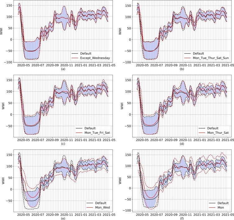
Examples of subsampling on the Reims WWTP, ranging from six days (top left) to one day per week (bottom right). Dotted lines represent the respective 95% prediction intervals for default (black) and subsampled (red) models. The default model uses all the available data from the Reims WWTP (usually 7 samples a week). Continuous lines show the WWI of both models. The blue-colored surface represents the intersection of both prediction intervals. The vertical grid corresponds to Mondays. On panel (d), short term trend of red and black signals differs early January. On panel (e), local peaks on early September and early December are missing on the subsampled signal. Subsampling can also induce couple days of time lags in peaks, as shown in panel (f) with both same local peaks.

We also used data from the Reims WWTP to compare different subsampled versions of the WWI with the incidence rate. We tested all combinations of two sampling days per week, excluding the possibility that sampling occurs on two consecutive days (a situation that can sometimes occur for logistical reasons, but should remain exceptional). This plant was not included in the second wave offset study in Section 3.4 due to logistical problems at that moment. So, we tested on the time period between November 30th 2020 and January 22nd 2021, where a peak is visible on both the incidence rate curve and the WWI curve. As the incidence data from Reims were not available for weekends and holidays, we revised the sampling rate upwards for the tests in this city as the number of points was lower (60% of the points compared to 50% for the studies focused on the second wave).

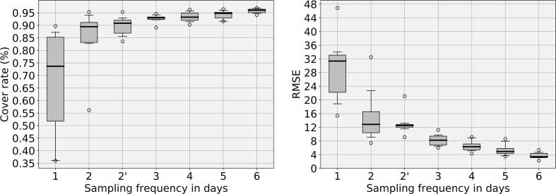
As shown in Fig. 9 and Fig. 10, subsampling does result in quite different curves. Such differences can have impacts on the evaluation of the time lag between the WWI and the incidence rate, as shown in Fig. 11 . We can see on Fig. 9 that both metrics show a clear improvement from once to twice a week sampling (RMSE is cut by more than half and median cover rate improves by 16%). Although the improvement weakens as the sampling frequency increases, it is important to note that the variance was also significantly reduced when moving from twice to three times a week.

Fig. 9.

Quantitative results of the sampling frequency analysis performed over the Reims WWTP. The left plot displays the evolution of the cover rate between 95% prediction intervals obtained with a reduced number of sampling days and the full signal. The cover rate represents the common surface of 95% prediction intervals between the default model and the studied subsampled model. The right plot shows the RMSE between the WWI. The x-axis represents the sampling frequency. 2’ frequency is a particular case of biweekly sampling where at least 2 days separate each sampling day (e.g. Monday can only be paired with Thursday or Friday). 3 days sampling seems to be the best cost-performance trade-off. 2’ solution still brings an improvement to simple 2 days sampling if 3 days sampling cannot be achieved.

Fig. 11.

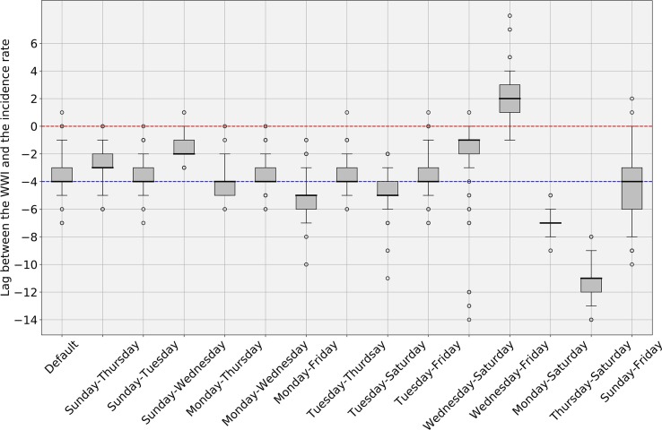
WWI and incidence rate lag estimates, in days, with varying sample days for the WWTP of Reims ($n=1000$ subsampling experiments with random sampling of 60% of incidence rate curve). Default corresponds to the WWI as it is routinely processed with every single data point available. Other possibilities are obtained through resampling twice a week on specific weekdays. The Red dotted line indicates the zero offset level. The Blue dotted line is the median level over the 14 medians. As the difference in variance between the set of median time lags from the 7 WWTPs of Fig. 7 and the set of median time lags from the 14 two-days combinations displayed here is not statistically significant, subsampling could be one of the factors explaining the variability in optimal time lags between WWTPs shown in Fig. 7.

Qualitative wise, we can see on Fig. 10 that going from 6 to 3 sampling days does not bring any significant difference to the WWI signal. Yet, short term interpretations can still be affected on specific periods as, the less sampling days available, the more biased towards outliers the WWI can become. Such a situation can be seen on Fig. 10 (d): while the default signal is continuously dwindling from early to mid-January, the subsampled signal is actually shortly going down, then increasing towards a plateau. Even though the general dynamics of the signal are still captured by once and twice a week sampling, local variations can be missed. On Fig. 10 (e), local peaks on early September and late November are missing on the subsampled signal. They are captured through once a week sampling, but with a slight offset.

Fig. 11 shows that a similar variance as the inter-WWTP variance shown in Fig. 7 can be observed by changing the sampling days of the same WWTP (the experiments were conducted on the Reims WWTP). Indeed, the difference in variance between the two sets of median time lags from the 7 WWTPs of Fig. 7 and the 14 two-days combinations of Fig. 11 is not statistically significant (p-value = 0.78). The difference in time lags observed in Fig. 7 between the 7 WWTPs studied could thus be notably explained by the approximation on the WWI signal because of subsampling.

The results of this subsampling study are therefore consistent with those of (Huisman et al., 2021): subsampling up to 3 days per week yields results that are substantially similar to daily sampling. Below this frequency, the representativeness of the results depends on the days chosen for sampling. Furthermore, decreasing the sampling frequency to one day per week has a significant impact on the representativeness of the signal compared to daily sampling, which is consistent with previous findings (Graham et al., 2020).

3.6. Assessment of the comparative ability of the WWI

The WWI was designed to make comparable the analysis results provided by different laboratories, each with its own analysis bias. These plants may process very different volumes of water with varying proportions of water from households, rainfall runoff, and other sources. In order to verify that this objective of uniformity is indeed achieved, we studied further the relationship between the WWI and a so-called reference indicator of the virus circulation derived from the incidence rate, which is considered as having a good comparative ability. If the objective of uniformity is reached, we expect this relationship to be the same whichever plant is considered.

To test the achievement of the uniformity objective, we consider the following 3 nested linear mixed effects models of increasing complexity:

• •
  The first one is the simple linear model (Model 0) which corresponds to the case when the homogeneity objective is fully fulfilled:

  $${\mathrm{WWI}}_{i,t}=\iota +\gamma Z_{i,t}+{∊}_{i,t},{∊}_{i,t}\stackrel{i.i.d}{\sim }\mathcal{N}(0,s^2),$$ (Model 0)

  where ${\mathrm{WWI}}_{i,t}$ is the WWI value at time t for plant i, $Z_{i,t}$ is the corresponding reference indicator, $\iota \in \mathbb{R},\gamma \in \mathbb{R}$ (the intercept and the slope in the linear relation) and $s\in {\mathbb{R}}^{+}$ (the level of uncertainty of the relation) are parameters to be estimated.
• •
  The second one is a mixed effect model (Model 1) with a random effect on the intercept. It corresponds to the case when the homogeneity target is fulfilled with regard to the multiplicative relation with the reference indicator, but not with regard to the additive relation with the reference indicator:

  $${\mathrm{WWI}}_{i,t}=\iota +K_i+\gamma Z_{i,t}+{∊}_{i,t},{∊}_{i,t}\stackrel{i.i.d}{\sim }\mathcal{N}(0,s^2)$$ (Model1)

  $$K_i\stackrel{i.i.d}{\sim }\mathcal{N}(0,s_K^2),$$

  where, in addition to the terms of Model 0, $K_i$ is the intercept random effect for plant i and $s_K\in {\mathbb{R}}^{+}$ is a parameter to be estimated.
• •
  The third and last one is a mixed effects model with 2 random effects (Model 2). It corresponds to the case when the homogeneity target is not fulfilled with regard to the multiplicative relation nor with regard to the additive relation with the reference indicator:

  $${\mathrm{WWI}}_{i,t}=\iota +K_i+(\gamma +G_i)Z_{i,t}+{∊}_{i,t},{∊}_{i,t}\stackrel{i.i.d}{\sim }\mathcal{N}(0,s^2)$$ (Model2)

  $$\left(\begin{array}{c}\hfill K_i\hfill \\ \hfill G_i\hfill \\ \hfill \hfill \end{array}\right)\stackrel{i.i.d}{\sim }\mathcal{N}\left(0,\left(\begin{array}{cc}\hfill s_K^2\hfill & \hfill s_{\mathit{KG}}\hfill \\ \hfill s_{\mathit{KG}}\hfill & \hfill s_G^2\hfill \\ \hfill \hfill \end{array}\right)\right),$$

  where, in addition to the terms of Model 1, $s_{\mathit{KG}}\in \mathbb{R}$ and $s_G\in {\mathbb{R}}^{+}$ are parameters to be estimated and $G_i$ is the slope random effect of plant i.

In the study that follows, the reference indicator, Z, is the logarithm of the incidence rate of the geographic area connected to the treatment plant considered at the same date. This indicator is considered as a good indicator by the sanitary authorities. The logarithmic transformation makes it possible to find a linear growth like the one obtained for the WWI and thus a comparable curve shape. This reference indicator can be assumed to be universal when it is not affected by public health policies or population movements, for example. We thus restrict the study to the so-called second wave of the epidemic in France excluding main holiday periods, from September the $1^{\mathit{st}}$, 2020 to December the ${15}^{\mathit{th}}$, 2020.

We estimated a time lag between the two indicators the same way we did in Section 3.4, and temporally realigned them accordingly. The focus is on all WWTPs which were analyzed at that time and for which the incidence rate is available for the related municipalities, even though the surveyed populations are not always exactly the same, but they are considered close enough. To learn the model parameters, we only use the points for which we have measurements at the WWTPs. This notably permits to measure the gain in comparative ability along the successive stages of the WWI construction.

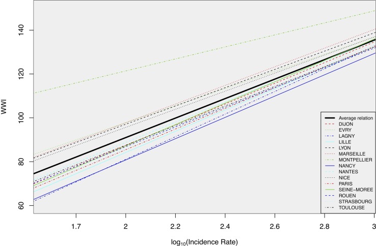
Fig. 12 shows the relation between the WWI and the incidence rate in log scale from the full mixed effects model (Model 2). Among the WTTPs considered for the training of the models, one has a stronger negative impact on the comparative ability of the WWI than the others, Montpellier-Maera, with an intercept significantly higher than the ones of the other WWTPs, resulting in a potential positive bias. The difference could partly be explained by the fact that the related laboratory, Lab 5, only treats this WWTP and two close cities, which complicates the automatic recalibration of this laboratory with regard to the other laboratories as it cannot cover a wide range of the French territory. Note that this laboratory is also the only one to provide quantified results by dPCR.

Fig. 12.

Relation between the WWI and the incidence rate in log scale learned by the full mixed effects model (Model 2). Montpellier relation greatly deviates from the average one. The significant deviation in intercept for Montpellier is probably due to an insufficient coverage of the French territory by the relative laboratory of this WWTP. Note that this laboratory is also the only one to provide quantified results by dPCR. The WWTP of Paris Seine-Amont was used for the comparison with the Grand Paris incidence rate.

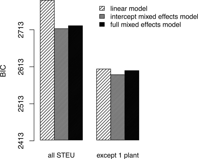
The results of models comparisons according to the Bayesian Information Criterion (BIC) are shown Fig. 13 . The lower the BIC, the better the performance of the evaluated model. The universal nature of the WWI is validated for the multiplier coefficient (higher performance of Model 1 compared to Model 2). If, in addition, the Montpellier-Maera sewage plant is excluded, comparative ability is greatly improved (performance of the mixed-effects models and of the simple linear model are closer), although the difference in performance remains significant and in favor of the intercept mixed-effect model (Model 1).

Fig. 13.

Comparison of Model 2 (full mixed effects model), Model 1 (intercept-only mixed effects model) and Model 0 (simple linear model) according to the Bayesian Information Criterion (BIC) before and after excluding one deviating WWTP (Montpellier-Maera). The lower the BIC is, the better the corresponding model is. Model 1 is thus selected while Model 2 is excluded.

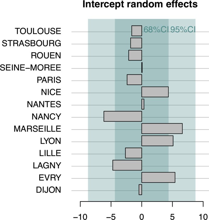
The (intercept) random effects learned with the selected model (Model 1) after removing the Montpellier-Maera WWTP are shown Fig. 14 . They correspond to the deviation of the WWI of the considered WWTPs from the standard relation between the WWIs and the city incidence rates. A positive (resp. negative) intercept random effect means the WWI should be lowered (resp. increased) in order to reflect the epidemic state in the same way that the incidence rate does. The deviations at most shortly exceed 5 units of the WWI: for Nancy, Lagny-sur-Marne (negative intercept effects), Marseille, Lyon and Evry (positive intercept effects) which is acceptable, the WWI typically ranging from −50 to 150.

Fig. 14.

Intercept random effects for Model 1 during the second wave of the epidemic for 14 WWTPs. A positive (resp. negative) intercept effect means the WWI should be lowered (resp. increased) in order to reflect the epidemic state in the same way that the incidence rate does. The deviations at most shortly exceed 5 units of the WWI: for Nancy, Lagny-sur-Marne (negative intercept effect), Marseille, Lyon, and Evry (positive intercept effects) which is acceptable, the WWI typically ranging from −50 to 150. The WWTP of Paris Seine-Amont was used for the comparison with the Grand Paris incidence rate.

As it stands, the objective of uniformity is not achieved, but likelihood ratio tests between the nested models show that the comparative ability is improved by each stage of the WWI construction. Indeed, the p-values for the comparison of the mixed effects model on the intercept (Model 1) with the simple linear model (Model 0) (after exclusion of the Montpellier-Maera WWTP) strongly increases as we move from the raw data (measurements performed at the WWTP, p-value of ${5.10}^{-34}$) to the data accounting for the inlet volumes and de-noised by the previously described smoother (p-value of ${9.10}^{-12}$) and to the WWI (p-value of ${4.10}^{-6}$).

4. Discussion

We have proposed an innovative approach to solve some inherent shortcomings of SARS-CoV-2 analysis in WWTP as a tool to evaluate COVID-19 epidemic. The present algorithm was used in the context of Obépine, a French national surveillance network that is monitoring viral load in 168 WWTPs as of August 26, 2020. The relevance of WBE as a decision support tool (Baldovin et al., 2021, Prado et al., 2021) has been concretely demonstrated in this project. This algorithm allows reducing the measurement noise by 17% and taking into account the deviations of quantification between different laboratories. It also makes it possible to consider the variations of flow at the inlet of the WWTP, among which the effects of dilutions due to rainfalls, regardless of the size of the WWTP. The signal resulting from this modeling is strongly correlated to the incidence signal in exponential regime, which is consistent with the results of (Wu et al., 2022, Wurtzer et al., 2020, Hata et al., 2021, D’Aoust et al., 2021, Medema et al., 2020, Ahmed et al., 2020, Peccia et al., 2020). Outside this regime, the correlation may be weaker, probably because the signal captured by the wastewater analyses is not limited to the detection of virus carriers by massive testing campaigns. Indeed, individual testing is most often restricted to symptomatic and contact cases and may not be representative of virus prevalence in people with no or mild symptoms, notably young people, as previously pointed out (Weidhaas et al., 2021). It has indeed been reported that asymptomatic patients may test positively for RT-qPCR in stools (Jiang et al., 2020, Tang et al., 2020, Park et al., 2021, Han et al., 2020, Quilliam et al., 2020), thus likely to be detected through wastewater analysis.

Based on the data at our disposal, three days sampling seems to be the optimal cost-performance trade-off to achieve similar results to a daily sampling frequency, and agrees with the conclusions of (Huisman et al., 2021). Although results seem already satisfying for twice a week sampling considering the same criterion and agrees with the conclusions of (Feng et al., 2021, Graham et al., 2020), chances are that some WWTPs are sampled at an inappropriate tuple of sample days. Thus, if the budget is not compatible with three days sampling, option 2’, corresponding to biweekly sampling with at least two days without sampling between each sample, might be the best compromise (see Fig. 10). Qualitative wise, we note that insufficient sampling frequency may lead to the failure to detect some events and affect short-term trends compared to a full week sampling. This is not surprising, as downgrading the sampling frequency reduces the information collected. One of the shortcomings of the subsampling study is that we did not have the opportunity to test all subsampling combinations for days prior to November, as the WWTP tested was not yet sampled every day at that time. We did not truncate from November for the study, for the reason of keeping a maximum of signal variability, especially the calm period of Summer 2020, when almost no significant viral concentrations were detected. Moreover, we were not able to replicate this subsampling experiment on another WWTP. The same study needs to be replicated on several WWTPs in order to generalize those results with higher reliability.

The results of estimated lags between the wastewater signals and the incidence rates are in the order of magnitude of a couple days during the exponential phase. Some plants show quite important lags compared to the others. For example, Nancy WWTP, where the WWI lags by 5 days on average and where the intra-experimental variance is more pronounced than in the other plants; or Paris Seine-Morée, where the WWI is 6 days ahead of the incidence rate signal. Several hypotheses seem plausible to explain these shifts. First, as shown in our downsampling experiment, biweekly sampling, although sufficient to capture the dynamics of the epidemic, may induce an additional uncertainty of a few days on the actual peak of excretion in wastewater. Furthermore, the signal captured in wastewater extends beyond simple reported positive cases. The propensity of populations to test themselves sometimes differs between EPCIs. For two metropolitan areas of similar size, such as Nancy and Mulhouse, the average screening rate during the third wave was more than 1.5 times higher in Nancy. In municipalities where people test particularly less or more than the average, the indicator is therefore more likely to be ahead or to lag behind the incidence by a few days. Finally, the good transposition capacity of the WWI from one WWTP to another, relative to what can be observed on the incidence rate signal, is to be considered. Even though it can still be worked upon, our study shows a significant improvement to this property thanks to our smoothing and normalization techniques. It should be noted that the more pronounced deviations in certain plants can have several explanations. For example, the incidence rate is only available for the whole of the Aix-Marseille agglomeration, which covers a much larger population than the only plant we monitor in the network in Marseille. The same applies to regional indicators, where the difference in correlation between the two regions could be explained by the deviation in surveyed populations. 28 WWTPs, with a nominal waterflow accounting for around 58% of the regional population, were followed in the Grand-Est region, while 7 were studied in the Île-de-France region (accounting for around 33% of the regional population), leading to a less accurate mesh.

4.1. Limitations

We are aware of the multiple shortcomings and uncertainties behind each stage of the formulation in Eq. 2, namely measurement errors on RNA regarding stage 1, poorly controlled outflow all along the network regarding stage 2, non-uniformity of human inputs to the sewer, processes in the sewer and variable additional industrial pollution flows with respect to stage 3. However, given the availability of data on a national scale, we consider this was the best feasible indicator.

Despite satisfying results, there is still room for improvement. About the inter-laboratory variability assessment, it would be much better to assess the different laboratories on large scale ILA with samples covering a wide range of values in log-scale. Yet, in view of the urgency of the epidemic situation in France from January 2021 and the need to quickly obtain models to help decision-making, the project moved into an action research phase. As such ILA results were not available at that time, the proposed modeling was considered as our best option. It shows a great improvement in reducing inter-laboratories variability as shown in Fig. 5. Yet, this normalization is not as effective as scaling from ILA results, notably because it is asymmetrical. The problem is that it was not possible to set $C_m$ as a minimum concentration value specific to each laboratory, as the true minimum values are censored by LOQs specific to each laboratory. Moreover, $C_m$ was originally designed to be the specific censoring threshold of each laboratory, so that the 0 level would correspond to this LOQ for each WWTP. However, one of the laboratories enrolled several months after the start of the project had a censoring threshold of 40 times the 1000 GU/L limit we are using for $C_m$ when he joined. Using a specific $C_m$ in the normalization step of the WWI would then have had greatly underestimated the epidemic situation for its related WWTPs. Finally, SARS-CoV-2 circulation level was high in France when we were asked to start communicating our results, hence we chose a normalization technique that would be more accurate for higher values, yet could still be improved for lower ones.

About the regional indicator, we chose not to use a simple average of the WWI to account for cases where very small WWTPs would then have a disproportionate weight in the regional signal. The downside of it is that it considers less of the aspect of the geographical diversity. For example, if two WWTPs are monitored in a region, with one in the north being really large and one in the south being quite small, the regional WWI will mostly reflect the northern status. An alternative to cope with this problem without extra cost would have been to cluster the clinical signals at city level and associate them with the WWI signals they had a strong correlation with in the same region. Then, the weighted average could have been computed not only with the population connected to each plant, but with the sum of the populations of the cities which clinical signals had a strong correlation with a WWI. Unfortunately, clinical signals not being openly available at a local level, such a modeling was not deemed possible.

Some of the intrinsic limitations of WBE still remain. Indeed, individual testing is more relevant to contact tracing process and more convenient for the ”tracking, testing, isolating” strategy set up by the French government. It can give faster results: from 30 min for an antigen test, to 24 h for a PCR test, rather than up to 3 days for the WBE treatment (24 h for sampling and up to 48 h for transport and analysis of the sample). Furthermore, positive cases are accurately identified when individual tests are done at a local scale, whereas WBE surveillance is an anonymising approach even at sewer level. Besides, dilution effects due to rainfall or civil engineering works may have a significant impact on raw PCR quantification. It is therefore important that the parameters for renormalizing these raw measurements, such as the flow rate at the station inlet, are available as soon as possible.

Despite significant improvements made on the intra- and inter-laboratory variance reduction, the WWI does not yet provide a perfect comparative ability. Indeed, a level of 100 in WWTP A and in WWTP B does not depict, as of today, the same epidemic situation, as shown in Fig. 12, Fig. 13, Fig. 14. However, the incidence rate, which is often considered as the clinical gold standard for case monitoring, presents similar limitations. Indeed, it still depends on the screening rate. As shown in Fig. B.1, the screening rate did vary in France between the second wave, during Autumn 2020, and the third wave, during Spring 2021. Furthermore, similar incidence levels can be found for very different screening rates in different departments, as shown in Table B.1. The more people are screened, the more positive cases are going to be found, and this screening rate is not the same when comparing different French departments. Among the usual clinical indicators, the hospitalization rate is one of the least biased. Yet, it still has the downside of only capturing severe cases. In addition, it always lags behind the other indicators.

On another note, improving confidence in the trends provided by the latest sampling is one of the major issues that still needs to be resolved about the WWI. Indeed, the goodness of the correction by the WWI of a point is more visible when compared both to its predecessors and successors. Such precision cannot be achieved for the very last value recorded, as there are no successors. Therefore, the levels and trends of the last 7 days may vary from week to week with new samples acquired. This problem is inherent to any smoothing technique and is exaggerated by low sampling rates. Another limitation of the WWI is that the patterns and periods of excretion may be variant dependent. This could make it complex to compare circulation levels between two different periods when the dominant variants were different. We found no studies addressing fecal shedding in patients infected with the delta variant, whereas several have addressed this issue for older strains (Wölfel et al., 2020, Wang et al., 2020, Lui et al., 2020). Modeling work has attempted to infer excretion curves from these data (Hoffmann and Alsing, 2021), or directly from wastewater data and daily cases (Petala et al., 2022, Cavany et al., 2021). However, it is important to have more information on the excretion dynamics in the stool of patients infected with the delta variant. Recent work has been done on this topic to compare viral loads of infected patients, with and without vaccine coverage (Acharya et al., 2021). Initial results indicate that no significant differences were found between the two groups, regardless of whether patients had symptoms of the infection. Yet, the same study does not include analysis of stool samples and does not present a longitudinal analysis of patients, as may have been done previously (Wölfel et al., 2020), which is required for the deconvolution of the signal.

On another topic, the EDQPI 3 formula assumes that the different physico-chemical indicators have the same accuracy to estimate household flow more accurately, as a simple average is used. Some works conclude that there is no significant difference in the estimation of populations by ammonium, COD, or flow measured at the plant inlet (Tscharke et al., 2019). However, the same study also indicates that ammonium would not be subject to the same variability as COD with respect to external factors of variability, implying greater variability in measurement from day to day. These variability factors include industrial or agricultural discharges, as well as infiltrations and exfiltrations (Been et al., 2014, Daughton, 2012). Further work is therefore needed on the accuracy of this normalization, for example by using a weighted normalization that takes into account both the accuracy and variability of the indicators selected for the watershed population estimate. The variability parameter has already been taken into account in recent works (Wade et al., 2022) but, to our knowledge, the differences in accuracy have not been subjected to a weighting. One last point on this topic, the WWI does not currently allow for normalization of data by taking into account differences in external discharges to household water in two different WWTPs. For example, if 20% of the flow in WWTP A comes from industrial discharges while this share is 40% in WWTP B, assuming that the flows in WWTPs A and B are the same, an additional dilution is brought to the quantitative results of WWTP B and is currently not corrected. This is part of ongoing research and should greatly improve the ability to compare indicator levels between WWTPs.

Besides, the scale of the indicator, varying from 0 to 150, is arbitrary. It has been defined during the still on-going study of a proper digital twin of the infected population. The idea remains to evolve this indicator on several levels. First, by using a deconvolution of a realistic excretion curve, which allows inferring a number of infected persons from the wastewater records. Then, by normalizing not to arbitrary thresholds, but to incidence levels. Such normalization would provide a scale more comparable to clinical data. The first point is a line of research that we continue to work on using our data. The second point cannot be developed because of restricted access to these clinical data. Such standardization could only be implemented for 21 monitored WWTPs as of November 9, 2021.

4.2. Strengths

Individual testing faces limitations that do not hinder WBE. In France, individual test results are reported by city of residence and not by city where the test was performed. As a result, the incidence rate is affected by population movements, particularly during vacation periods, whereas WBE does not have this bias. Moreover, individual testing still depends on the willingness of a population to get tested and to report all their contact cases. In this sense, WBE is closer to a mass screening, and is non-invasive as well. Finally, individual testing is most often limited to symptomatic cases, whereas the WWI also allows detection of asymptomatic cases. The joint use of WBE and individual testing is the standard towards which we should strive.

Another strength of the WWI is that it is far less costly than massive individual testing (Hart and Halden, 2020). From sampling to transportation to analysis, the cost of quantifying one sample is €210 for the WWI. In France, as of November 4, 2021, individual test costs vary from €22 (antigen tests) to €44 (PCR tests). Based on two samples per week and 168 WWTPs, WWI allows mass screening of 33% of the French population, at a global cost of €70,000 per week. The same screening, performed on individuals, with two antigen tests per individual and per week, would cost €990,000,000. In addition, the waiting time for individual results would be much longer than it is now due to the logistical limitations that such a campaign would imply, not to mention possible reagent shortages that could occur with such a high demand. Furthermore, public acceptance of such a testing campaign would not be guaranteed. The WWI could then be used routinely for mass screening purposes and as an incentive for increasing individual mass testing on specific locations when the epidemic situation begins to deteriorate.

Despite the improvements that can still be made to the WWI, we have nevertheless presented a new and original approach. This approach addresses the problem of inter-laboratory variability, when the results of ILA, although indispensable (Ahmed et al., 2022), are not yet available. In addition, the method used for data smoothing allows the detection of outliers and the consideration of censoring thresholds specific to the LOQs of the different laboratories. The method thus achieves a correlation gain of 18% with the incidence rate, compared to what would be obtained by using only the raw PCR quantification results. In addition, the WWI makes it possible to aggregate the results of the different WWTPs and to obtain a regional indicator consistent with the clinical data. Finally, in France, as of November 9, 2021, clinical data at the urban unit level are available to the general public for only 22 EPCIs. Our indicator allows to inform the largest number of people about the status of the epidemic at a finer granularity than the departmental scale, which is the most accurate available in open access. However, additional research is needed on small WWTPs to ensure that the clinical data still correlates well with the WWI.

5. Conclusion

The underlying signal in wastewater measurements of SARS-CoV-2 faithfully reflects the dynamics of the epidemic and has the advantage of being unbiased by test availability, willingness of populations to be tested, and population movements. In certain periods, the WWI is also more faithful to the true epidemic situation than the incidence rate, which is obtained as a rolling week average and is therefore very sensitive to holidays (uncharacteristic collapse of the epidemic situation at the peak of the third wave of the pandemic on the incidence rate signal). Moreover, the measurement of this epidemic signal in wastewater proves to be much less costly than massive individual testing. Indeed, it allows obtaining a signal strongly correlated to the more usual epidemic indicators by requiring a single analysis to reflect the average epidemic situation of thousands of people. Finally, this indicator provides an unbiased survey of the infected population, as it also integrates the contribution of asymptomatic infected persons, which is only partially reflected in the positive test reports, and of unreported infection cases. The signal that emerges from these analyses is strongly correlated with the incidence rate and we consider it to be a credible complementary approach to the latter, as its relevance could decline in a few months with the advance of the vaccination campaign and therefore a likely reduction in the quantity of tests carried out to monitor the epidemic.

6. Data sources

6.1. WWI

WWTP based and region based WWI data can be found here. Analysis reports are also available here.

6.2. Incidence rate

Incidence rate data are partially available in open access for 22 Etablissement Public de Coopération Intercommunale (EPCI) and can be found here. Incidence data are built on both qPCR nasopharyngeal swabs and antigen tests. More detailed information about this data can be found here. For the Grand Reims metropolitan area, incidence data are not available in open access. We have retrieved them by studying the different dashboards issued by the ARS Grand-Est (example here). For three additional plants (Lagny-sur-Marne, Evry and Paris Seine Morée), the data corresponding to the specific watershed of these plants were directly transmitted to us by Santé Publique France.

Declaration of Competing Interest

The authors declare that they have no known competing financial interests or personal relationships that could have appeared to influence the work reported in this paper.

Handling Editor: Frederic Coulon

Appendix A. Quantification results

Fig. A.1.

Fig. A.1.

Quantification results distributions by laboratory and by gene, in log scale. These distributions show clear disparities in censoring thresholds between laboratories. Lab 1 only quantified the E gene at the very beginning of its follow-up, which resulted in a more pronounced asymmetry of the high values.

Appendix B. Incidence and screening rates

Fig. B.1, Fig. B.2, Fig. B.3.

Fig. B.2.

Visualization of the WWI and the log of the incidence rate. The overall dynamics seem to match quite well, even beyond the period under study. Montpellier seems to differ from the other WTTPs, as discussed in Section 3.6. Lyon’s WWTP is La Feyssine (1/2).

Fig. B.3.

Visualization of the WWI and the log of the incidence rate. The overall dynamics seem to match quite well, even beyond the period under study. Nantes’s WWTP is Petite Californie (2/2).

Table B.1.

Table B.1.

7-day averages, centered on the second wave peak in France, for incidence and screening rates. Several examples suggest that the incidence rate may not accurately represent the same populations of infected individuals. For example, departments 01 and 08 have very similar screening rates (difference of 0.95%), but very different incidence rates (difference of 44%). Departments 76 and 77 have a similar incidence rate (difference of 0%) but different screening rates (difference of 23%).

Dep	Incidence	Screening	Dep	Incidence	Screening	Dep	Incidence	Screening
01	936	3838	33	247	2274	66	386	3615
02	333	2599	34	475	3429	67	596	4936
03	586	4015	35	314	2502	68	450	3484
04	450	3031	36	282	2438	69	913	4222
05	726	3003	37	391	3141	70	483	3285
06	364	2893	38	914	3494	71	704	4024
07	737	3434	39	725	4093	72	294	2586
08	526	3875	40	338	2981	73	1160	3751
09	347	3211	41	304	2338	74	1141	3892
10	449	2984	42	1194	4861	75	600	4165
11	330	3503	43	1111	4006	76	433	2928
12	498	4239	44	364	2797	77	433	2248
13	601	4564	45	492	3527	78	481	2646
14	371	2991	46	213	2368	79	315	3203
15	323	3018	47	300	2728	80	304	2665
16	219	2330	48	617	3241	81	454	3201
17	156	2017	49	433	3112	82	417	2923
18	446	2818	50	218	2356	83	528	4081
19	319	3268	51	386	2699	84	716	3758
21	565	3581	52	560	3604	85	301	2921
22	217	2463	53	386	2400	86	323	3290
23	443	4275	54	429	3894	87	381	3083
24	312	3220	55	378	3038	88	448	3429
25	751	3778	56	202	2019	89	522	3462
26	717	3522	57	449	3733	90	503	3449
27	357	2281	58	364	3361	91	485	2663
28	327	2349	59	819	5009	92	546	3575
29	190	2423	60	472	2907	93	521	2471
2A	495	4283	61	325	2552	94	537	3031
2B	327	4085	62	583	4012	95	601	2907
30	615	3367	63	553	3781
31	401	3067	64	526	4271
32	263	2562	65	524	3648

References

- Acharya C.B., Schrom J., Mitchell A.M., Coil D.A., Marquez C., Rojas S., Wang C.Y., Liu J., Pilarowski G., Solis L., Georgian E., Petersen M., DeRisi J., Michelmore R., Havlir D. No Significant Difference in Viral Load Between Vaccinated and Unvaccinated, Asymptomatic and Symptomatic Groups When Infected with SARS-CoV-2 Delta Variant. medRxiv. 2021 doi: 10.1101/2021.09.28.21264262. [DOI] [PMC free article] [PubMed] [Google Scholar]
- Ahmed W., Angel N., Edson J., Bibby K., Bivins A., O’Brien J.W., Choi P.M., Kitajima M., Simpson S.L., Li J., Tscharke B., Verhagen R., Smith W.J.M., Zaugg J., Dierens L., Hugenholtz P., Thomas K.V., Mueller J.F. First confirmed detection of SARS-CoV-2 in untreated wastewater in Australia: A proof of concept for the wastewater surveillance of COVID-19 in the community. Sci. Total Environ. 2020;728:138764. doi: 10.1016/j.scitotenv.2020.138764. [DOI] [PMC free article] [PubMed] [Google Scholar]
- Ahmed W, Simpson S.L., Bertsh P.M., Bibby K., Bivins A., Blackall L.L., Bofill-Mas S., Bosch A., Brandão J., Choi P.M., Ciesielski M., Donner E., D’Souza N., Farnleitner A.H., Gerrity D., Gonzalez R., Griffith J.F., Gyawali P., Haas C.N., Hamilton K.A., Hapuarachchi H.C., Harwood V.J., Haque R., Jackson G., Khan S.J., Khan W., Kitajima M., Korajkic A., La Rosa G., Layton B.A., Lipp E., McLellan S.L., McMinn B., Medema G., Metcalfe S., Meijer W.G., Mueller J.F., Murphy H., Naughton C.C., Noble R.T., Payyappat S., Petterson S., Pitkänen T., Rajal V.B., Reyneke B., Roman F.A., Jr., Rose J.B., Rusiñol M., Sadowsky M.J., Sala-Comorera L., Setoh Y.X., Sherchan S.P., Sirikanchana K., Smith W., Steele J.A., Sabburg R., Symonds E.M., Thai P., Thomas K.V., Tynan J., Toze S., Thompson J., Whiteley A.S., Wong J.C.C., Sano D., Wuertz S., Xagoraraki I., Zhang Q., Zimmer-Faust A.G., Shanks O.C. Minimizing errors in RT-PCR detection and quantification of SARS-CoV-2 RNA for wastewater surveillance. Science of The Total Environment. 2022;805 doi: 10.1016/j.scitotenv.2021.149877. [DOI] [PMC free article] [PubMed] [Google Scholar]
- Ahmed W., Tscharke B., Bertsch P.M., Bibby K., Bivins A., Choi P., Clarke L., Dwyer J., Edson J., Nguyen T.M.H., O’Brien J.W., Simpson S.L., Sherman P., Thomas K.V., Verhagen R., Zaugg J., Mueller J.F. SARS-CoV-2 RNA monitoring in wastewater as a potential early warning system for COVID-19 transmission in the community: A temporal case study. Sci. Total Environ. 2021;761:144216. doi: 10.1016/j.scitotenv.2020.144216. [DOI] [PMC free article] [PubMed] [Google Scholar]
- Anand U., Adelodun B., Pivato A., Suresh S., Indari O., Jakhmola S., Jha H.C., Jha P.K., Tripathi V., Di Maria F. A review of the presence of SARS-CoV-2 RNA in wastewater and airborne particulates and its use for virus spreading surveillance. Environ. Res. 2021;196:110929. doi: 10.1016/j.envres.2021.110929. [DOI] [PMC free article] [PubMed] [Google Scholar]
- Baldovin T., Amoruso I., Fonzo M., Buja A., Baldo V., Cocchio S., Bertoncello C. SARS-CoV-2 RNA detection and persistence in wastewater samples: An experimental network for COVID-19 environmental surveillance in Padua, Veneto Region (NE Italy) Sci. Total Environ. 2021;760:143329. doi: 10.1016/j.scitotenv.2020.143329. [DOI] [PMC free article] [PubMed] [Google Scholar]
- Been F., Rossi L., Ort C., Rudaz S., Delémont O., Esseiva P. Population Normalization with Ammonium in Wastewater-Based Epidemiology: Application to Illicit Drug Monitoring. Environ. Sci. Technol. 2014;48:8162–8169. doi: 10.1021/es5008388. [DOI] [PubMed] [Google Scholar]
- Bertrand I., Challant J., Jeulin H., Hartard C., Mathieu L., Lopez S., Schvoerer E., Courtois S., Gantzer C. Epidemiological surveillance of SARS-CoV-2 by genome quantification in wastewater applied to a city in the northeast of France: Comparison of ultrafiltration- and protein precipitation-based methods. Int. J. Hygiene and Environ. Health. 2021;233:113692. doi: 10.1016/j.ijheh.2021.113692. [DOI] [PMC free article] [PubMed] [Google Scholar]
- Bivins A., Kaya D., Bibby K., Simpson S., Bustin S., Shanks O., Ahmed W. Inherent Bias of SARS-CoV-2 RNA Quantification for Wastewater Surveillance Due to Variable RT-qPCR Assay Parameters. MDPI AG. 2021 doi: 10.20944/preprints202106.0320.v1. [DOI] [PMC free article] [PubMed] [Google Scholar]
- Cavany S., Bivins A., Wu Z., North D., Bibby K., Perkins T.A. Inferring SARS-CoV-2 RNA shedding into wastewater relative to time of infection. medRxiv. 2021 doi: 10.1101/2021.06.03.21258238. [DOI] [PMC free article] [PubMed] [Google Scholar]
- Courbariaux M., Cluzel N., Wang S., Maréchal V., Moulin L., Wurtzer S., Obépine consortium, Mouchel J., Maday Y., Nuel G. An autoregressive model for a censored data denoising method robust to outliers with application to the Obépine SARS-Cov-2 monitoring. arXiv. 2021 https://arxiv.org/abs/2108.02115. [Google Scholar]
- D’Aoust P.M., Graber T.E., Mercier E., Montpetit D., Alexandrov I., Neault N., Baig A.T., Mayne J., Zhang X., Alain T., Servos M.R., Srikanthan N., MacKenzie M., Figeys D., Manuel D., Jüni P., MacKenzie A.E., Delatolla R. Catching a resurgence: Increase in SARS-CoV-2 viral RNA identified in wastewater 48 h before COVID-19 clinical tests and 96 h before hospitalizations. Sci. Total Environ. 2021;770:145319. doi: 10.1016/j.scitotenv.2021.145319. [DOI] [PMC free article] [PubMed] [Google Scholar]
- D’Aoust P.M., Mercier E., Montpetit D., Jia J.-J., Alexandrov I., Neault N., Baig A.T., Mayne J., Zhang X., Alain T., Langlois M.-A., Servos M.R., MacKenzie M., Figeys D., MacKenzie A.E., Graber T.E., Delatolla R. Quantitative analysis of SARS-CoV-2 RNA from wastewater solids in communities with low COVID-19 incidence and prevalence. Water Research. 2021;188:116560. doi: 10.1016/j.watres.2020.116560. [DOI] [PMC free article] [PubMed] [Google Scholar]
- Daughton C.G. Real-time estimation of small-area populations with human biomarkers in sewage. Sci. Total Environ. 2012;414:6–21. doi: 10.1016/j.scitotenv.2011.11.015. [DOI] [PubMed] [Google Scholar]
- Feng S., Roguet A., McClary-Gutierrez J.S., Newton R.J., Kloczko N., Meiman J.G., McLellan S.L. Evaluation of Sampling, Analysis, and Normalization Methods for SARS-CoV-2 Concentrations in Wastewater to Assess COVID-19 Burdens in Wisconsin Communities. ACS EST Water. 2021;1:1955–1965. doi: 10.1021/acsestwater.1c00160. [DOI] [Google Scholar]
- Fernandez-Cassi X., Scheidegger A., Bänziger C., Cariti F., Corzon A.T., Ganesanandamoorthy P., Lemaitre J.C., Ort C., Julian T.R., Kohn T. Wastewater monitoring outperforms case numbers as a tool to track COVID-19 incidence dynamics when test positivity rates are high. medRxiv. 2021 doi: 10.1101/2021.03.25.21254344. [DOI] [PMC free article] [PubMed] [Google Scholar]
- Fraser D., Potter J. The optimum linear smoother as a combination of two optimum linear filters. IEEE Trans. Automat. Contr. 1969;14:387–390. doi: 10.1109/tac.1969.1099196. [DOI] [Google Scholar]
- Gandhi M., Yokoe D.S., Havlir D.V. Asymptomatic Transmission, the Achilles’ Heel of Current Strategies to Control Covid-19. N Engl J Med. 2020;382:2158–2160. doi: 10.1056/nejme2009758. [DOI] [PMC free article] [PubMed] [Google Scholar]
- Graham K.E., Loeb S.K., Wolfe M.K., Catoe D., Sinnott-Armstrong N., Kim S., Yamahara K.M., Sassoubre L.M., Mendoza Grijalva L.M., Roldan-Hernandez L., Langenfeld K., Wigginton K.R., Boehm A.B. SARS-CoV-2 RNA in Wastewater Settled Solids Is Associated with COVID-19 Cases in a Large Urban Sewershed. Environ. Sci. Technol. 2020;55:488–498. doi: 10.1021/acs.est.0c06191. [DOI] [PubMed] [Google Scholar]
- Han M.S., Seong M.-W., Kim N., Shin S., Cho S.I., Park H., Kim T.S., Park S.S., Choi E.H. Viral RNA Load in Mildly Symptomatic and Asymptomatic Children with COVID-19, Seoul, South Korea. Emerg. Infect. Dis. 2020;26:2497–2499. doi: 10.3201/eid2610.202449. [DOI] [PMC free article] [PubMed] [Google Scholar]
- Hart O.E., Halden R.U. Computational analysis of SARS-CoV-2/COVID-19 surveillance by wastewater-based epidemiology locally and globally: Feasibility, economy, opportunities and challenges. Sci. Total Environ. 2020;730:138875. doi: 10.1016/j.scitotenv.2020.138875. [DOI] [PMC free article] [PubMed] [Google Scholar]
- Hata A., Hara-Yamamura H., Meuchi Y., Imai S., Honda R. Detection of SARS-CoV-2 in wastewater in Japan during a COVID-19 outbreak. Sci. Total Environ. 2021;758:143578. doi: 10.1016/j.scitotenv.2020.143578. [DOI] [PMC free article] [PubMed] [Google Scholar]
- Hoffmann T., Alsing J. Faecal shedding models for SARS-CoV-2 RNA amongst hospitalised patients and implications for wastewater-based epidemiology. medRxiv. 2021 doi: 10.1101/2021.03.16.21253603. [DOI] [Google Scholar]
- Huisman J.S., Scire J., Caduff L., Fernandez-Cassi X., Ganesanandamoorthy P., Kull A., Scheidegger A., Stachler E., Boehm A.B., Hughes B., Knudson A., Topol A., Wigginton K.R., Wolfe M.K., Kohn T., Ort C., Stadler T., Julian T.R. Wastewater-based estimation of the effective reproductive number of SARS-CoV-2. medRxiv. 2021 doi: 10.1101/2021.04.29.21255961. [DOI] [PMC free article] [PubMed] [Google Scholar]
- Jiang X., Luo M., Zou Z., Wang X., Chen C., Qiu J. Asymptomatic SARS-CoV-2 infected case with viral detection positive in stool but negative in nasopharyngeal samples lasts for 42 days. J Med Virol. 2020;92:1807–1809. doi: 10.1002/jmv.25941. [DOI] [PMC free article] [PubMed] [Google Scholar]
- Kantor R.S., Nelson K.L., Greenwald H.D., Kennedy L.C. Challenges in Measuring the Recovery of SARS-CoV-2 from Wastewater. Environ. Sci. Technol. 2021;55:3514–3519. doi: 10.1021/acs.est.0c08210. [DOI] [PubMed] [Google Scholar]
- Kocamemi B.A., Kurt H., Hacıoglu S., Yaralı C., Saatci A.M., Pakdemirli B. First Data-Set on SARS-CoV-2 Detection for Istanbul Wastewaters in Turkey. medRxiv. 2020 doi: 10.1101/2020.05.03.20089417. [DOI] [Google Scholar]
- Krivoňáková N., Šoltýsová A., Tamáš M., Takáč Z., Krahulec J., Ficek A., Gál M., Gall M., Fehér M., Krivjanská A., Horáková I., Belišová N., Bímová P., Škulcová A.B., Mackuľak T. Mathematical modeling based on RT-qPCR analysis of SARS-CoV-2 in wastewater as a tool for epidemiology. Sci Rep. 2021;11 doi: 10.1038/s41598-021-98653-x. [DOI] [PMC free article] [PubMed] [Google Scholar]
- Lui G., Ling L., Lai C.K., Tso E.Y., Fung K.S., Chan V., Ho T.H., Luk F., Chen Z., Ng J.K., Chow K., Cheng P.K., Chan R.C., Tsang D.N., Gomersall C.D., Hui D.S., Chan P.K. Viral dynamics of SARS-CoV-2 across a spectrum of disease severity in COVID-19. Journal of Infection. 2020;81:318–356. doi: 10.1016/j.jinf.2020.04.014. [DOI] [PMC free article] [PubMed] [Google Scholar]
- Mayne D.Q. A solution of the smoothing problem for linear dynamic systems. Automatica. 1966;4:73–92. doi: 10.1016/0005-1098(66)90019-7. [DOI] [Google Scholar]
- Medema G., Heijnen L., Elsinga G., Italiaander R., Brouwer A. Presence of SARS-Coronavirus-2 RNA in Sewage and Correlation with Reported COVID-19 Prevalence in the Early Stage of the Epidemic in The Netherlands. Environ. Sci. Technol. Lett. 2020;7:511–516. doi: 10.1021/acs.estlett.0c00357. [DOI] [PubMed] [Google Scholar]
- Mizumoto K., Kagaya K., Zarebski A., Chowell G. Estimating the asymptomatic proportion of coronavirus disease 2019 (COVID-19) cases on board the Diamond Princess cruise ship, Yokohama, Japan, 2020. Eurosurveillance. 2020;25 doi: 10.2807/1560-7917.es.2020.25.10.2000180. [DOI] [PMC free article] [PubMed] [Google Scholar]
- Nelder J.A., Mead R. A Simplex Method for Function Minimization. The Computer Journal. 1965;7:308–313. doi: 10.1093/comjnl/7.4.308. [DOI] [Google Scholar]
- Park S., Lee C.-W., Park D.-I., Woo H.-Y., Cheong H.S., Shin H.C., Ahn K., Kwon M.-J., Joo E.-J. Detection of SARS-CoV-2 in Fecal Samples From Patients With Asymptomatic and Mild COVID-19 in Korea. Clinical Gastroenterology and Hepatology. 2021;19:1387–1394.e2. doi: 10.1016/j.cgh.2020.06.005. [DOI] [PMC free article] [PubMed] [Google Scholar]
- Peccia J., Zulli A., Brackney D.E., Grubaugh N.D., Kaplan E.H., Casanovas-Massana A., Ko A.I., Malik A.A., Wang D., Wang M., Warren J.L., Weinberger D.M., Arnold W., Omer S.B. Measurement of SARS-CoV-2 RNA in wastewater tracks community infection dynamics. Nat Biotechnol. 2020;38:1164–1167. doi: 10.1038/s41587-020-0684-z. [DOI] [PMC free article] [PubMed] [Google Scholar]
- Petala M., Kostoglou M., Karapantsios Th., Dovas C.I., Lytras Th., Paraskevis D., Roilides E., Koutsolioutsou-Benaki A., Panagiotakopoulos G., Sypsa V., Metallidis S., Papa A., Stylianidis E., Papadopoulos A., Tsiodras S., Papaioannou N. Relating SARS-CoV-2 shedding rate in wastewater to daily positive tests data: A consistent model based approach. Sci. Total Environ. 2022;807:150838. doi: 10.1016/j.scitotenv.2021.150838. [DOI] [PMC free article] [PubMed] [Google Scholar]
- Prado T., Fumian T.M., Mannarino C.F., Resende P.C., Motta F.C., Eppinghaus A.L.F., Chagas do Vale V.H., Braz R.M.S., da Silva Ribeiro de Andrade J., Maranhão A.G., Miagostovich M.P. Wastewater-based epidemiology as a useful tool to track SARS-CoV-2 and support public health policies at municipal level in Brazil. Water Research. 2021;191:116810. doi: 10.1016/j.watres.2021.116810. [DOI] [PMC free article] [PubMed] [Google Scholar]
- Quilliam R.S., Weidmann M., Moresco V., Purshouse H., O’Hara Z., Oliver D.M. COVID-19: The environmental implications of shedding SARS-CoV-2 in human faeces. Environment International. 2020;140:105790. doi: 10.1016/j.envint.2020.105790. [DOI] [PMC free article] [PubMed] [Google Scholar]
- Rauch H.E., Tung F., Striebel C.T. Maximum likelihood estimates of linear dynamic systems. AIAA Journal. 1965;3:1445–1450. doi: 10.2514/3.3166. [DOI] [Google Scholar]
- Saguti F., Magnil E., Enache L., Churqui M.P., Johansson A., Lumley D., Davidsson F., Dotevall L., Mattsson A., Trybala E., Lagging M., Lindh M., Gisslén M., Brezicka T., Nyström K., Norder H. Surveillance of wastewater revealed peaks of SARS-CoV-2 preceding those of hospitalized patients with COVID-19. Water Research. 2021;189:116620. doi: 10.1016/j.watres.2020.116620. [DOI] [PMC free article] [PubMed] [Google Scholar]
- Tang A., Tong Z., Wang H., Dai Y., Li K., Liu J., Wu W., Yuan C., Yu M., Li P., Yan J. Detection of Novel Coronavirus by RT-PCR in Stool Specimen from Asymptomatic Child, China. Emerg. Infect. Dis. 2020;26:1337–1339. doi: 10.3201/eid2606.200301. [DOI] [PMC free article] [PubMed] [Google Scholar]
- Tscharke B.J., O’Brien J.W., Ort C., Grant S., Gerber C., Bade R., Thai P.K., Thomas K.V., Mueller J.F. Harnessing the Power of the Census: Characterizing Wastewater Treatment Plant Catchment Populations for Wastewater-Based Epidemiology. Environ. Sci. Technol. 2019;53:10303–10311. doi: 10.1021/acs.est.9b03447. [DOI] [PubMed] [Google Scholar]
- Wade M.J., Lo Jacomo A., Armenise E., Brown M.R., Bunce J.T., Cameron G.J., Fang Z., Farkas K., Gilpin D.F., Graham D.W., Grimsley J.M.S., Hart A., Hoffmann T., Jackson K.J., Jones D.L., Lilley C.J., McGrath J.W., McKinley J.M., McSparron C., Nejad B.F., Morvan M., Quintela-Baluja M., Roberts A.M.I., Singer A.C., Souque C., Speight V.L., Sweetapple C., Walker D., Watts G., Weightman A., Kasprzyk-Hordern B. Understanding and managing uncertainty and variability for wastewater monitoring beyond the pandemic: Lessons learned from the United Kingdom national COVID-19 surveillance programmes. Journal of Hazardous Materials. 2022;424:127456. doi: 10.1016/j.jhazmat.2021.127456. [DOI] [PMC free article] [PubMed] [Google Scholar]
- Wang W., Xu Y., Gao R., Lu R., Han K., Wu G., Tan W. Detection of SARS-CoV-2 in Different Types of Clinical Specimens. JAMA. 2020 doi: 10.1001/jama.2020.3786. [DOI] [PMC free article] [PubMed] [Google Scholar]
- Weidhaas J., Aanderud Z.T., Roper D.K., VanDerslice J., Gaddis E.B., Ostermiller J., Hoffman K., Jamal R., Heck P., Zhang Y., Torgersen K., Laan J.V., LaCross N. Correlation of SARS-CoV-2 RNA in wastewater with COVID-19 disease burden in sewersheds. Sci. Total Environ. 2021;775:145790. doi: 10.1016/j.scitotenv.2021.145790. [DOI] [PMC free article] [PubMed] [Google Scholar]
- Wölfel R., Corman V.M., Guggemos W., Seilmaier M., Zange S., Müller M.A., Niemeyer D., Jones T.C., Vollmar P., Rothe C., Hoelscher M., Bleicker T., Brünink S., Schneider J., Ehmann R., Zwirglmaier K., Drosten C., Wendtner C. Virological assessment of hospitalized patients with COVID-2019. Nature. 2020;581:465–469. doi: 10.1038/s41586-020-2196-x. [DOI] [PubMed] [Google Scholar]
- Wu F., Xiao A., Zhang J., Moniz K., Endo N., Armas F., Bonneau R., Brown M.A., Bushman M., Chai P.R., Duvallet C., Erickson T.B., Foppe K., Ghaeli N., Gu X., Hanage W.P., Huang K.H., Lee W.L., Matus M., McElroy K.A., Nagler J., Rhode S.F., Santillana M., Tucker J.A., Wuertz S., Zhao S., Thompson J., Alm E.J. SARS-CoV-2 RNA concentrations in wastewater foreshadow dynamics and clinical presentation of new COVID-19 cases. Sci. Total Environ. 2022;805:150121. doi: 10.1016/j.scitotenv.2021.150121. [DOI] [PMC free article] [PubMed] [Google Scholar]
- Wurtzer S., Marechal V., Mouchel J., Maday Y., Teyssou R., Richard E., Almayrac J., Moulin L. Evaluation of lockdown effect on SARS-CoV-2 dynamics through viral genome quantification in waste water, Greater Paris, France, 5 March to 23 April 2020. Eurosurveillance. 2020;25 doi: 10.2807/1560-7917.es.2020.25.50.2000776. [DOI] [PMC free article] [PubMed] [Google Scholar]
- Xiao A., Wu F., Bushman M., Zhang J., Imakaev M., Chai P.R., Duvallet C., Endo N., Erickson T.B., Armas F., Arnold B., Chen H., Chandra F., Ghaeli N., Gu X., Hanage W.P., Lee W.L., Matus M., McElroy K.A., Moniz K., Rhode S.F., Thompson J., Alm E.J. Metrics to relate COVID-19 wastewater data to clinical testing dynamics. medRxiv. 2021 doi: 10.1101/2021.06.10.21258580. [DOI] [PMC free article] [PubMed] [Google Scholar]