Abstract
Deep learning-based video anomaly detection methods have drawn significant attention in the past few years due to their superior performance. However, almost all the leading methods for video anomaly detection rely on large-scale training datasets with long training times. As a result, many real-world video analysis tasks are still not applicable for fast deployment. On the other hand, the leading methods cannot provide interpretability due to the uninterpretable feature representations hiding the decision-making process when anomaly detection models are considered as a black box. However, the interpretability for anomaly detection is crucial since the corresponding response to the anomalies in the video is determined by their severity and nature. To tackle these problems, this paper proposes an efficient deep learning framework for video anomaly detection and provides explanations. The proposed framework uses pre-trained deep models to extract high-level concept and context features for training denoising autoencoder (DAE), requiring little training time (i.e., within 10 s on UCSD Pedestrian datasets) while achieving comparable detection performance to the leading methods. Furthermore, this framework presents the first video anomaly detection use of combing autoencoder and SHapley Additive exPlanations (SHAP) for model interpretability. The framework can explain each anomaly detection result in surveillance videos. In the experiments, we evaluate the proposed framework's effectiveness and efficiency while also explaining anomalies behind the autoencoder’s prediction. On the USCD Pedestrian datasets, the DAE achieved 85.9% AUC with a training time of 5 s on the USCD Ped1 and 92.4% AUC with a training time of 2.9 s on the UCSD Ped2.
Keywords: Security, Video surveillance, Anomaly video analysis, Abnormal event detection, Deep features, Context mining, Interpretability
Introduction
Security cameras are becoming widely used and powered with networking technologies, improved surveillance capabilities, and advancements in storage systems. It has been observed that the installation of surveillance cameras significantly reduces the crime rate. For example, the total crime in downtown Baltimore (Maryland, USA) reduced about a quarter in four months after installing the surveillance camera. Similarly, violent crime declined about 20% in Chicago (USA) [1]. Besides the public security field, surveillance cameras are also applied on business operations, health care, smart home applications, etc. The industry research HIS Markit reported that there existed approximately 770 million security cameras worldwide in 2019, and the total number of security cameras will increase to 1 billion before 2022 [2]. However, storing and manually evaluating a large amount of data from many surveillance cameras are no longer practical, which started the discussions and studies in anomaly detection in surveillance. Moreover, the detection using opaque models, such as the deep learning models, lacks explanations of how the model decides the results. Therefore, the interpretability of anomaly detection in the video has become a main challenge in the surveillance system. In this paper, the anomaly is defined as the abnormal behavior and event in the surveillance videos. The objective of explainable video anomaly detection is to autonomously detect an anomalous event in the video recording with supportive explanations (i.e., not only giving the result of if an anomaly occurs but also explaining why it is considered as an anomaly—current studies mainly focus on just detection without sufficient explanation).
Powered by the huge performance improvement of deep learning methods, many autoencoder-based video anomaly detection approaches have been studied in the last few years. For example, Appearance and Motion DeepNet (AMDN) [3] trained deep convolutional neural networks for processing the input raw RGB (Red, Green, Blue) image and the optical flow map. Two-Stream Variational AutoEncoder (VAE) [4] improves the detection accuracy by adapting the VAE. (Spatio-Temporal Adversarial Network) STAN [5] detects the anomaly by using the Generative Adversarial Network (GAN). For explaining the anomaly detection results, currently, many methods rely on highlighting the suspicious region without further description. For instance, the University of California San Diego (UCSD) Ped1 and Ped2 datasets provide pixel-level anomaly localization as the dataset. Some methods [3, 4, 6–8] not only show the frame-level anomaly detection but also shows the pixel-level anomaly detection result.
However, current approaches have faced a number of challenges. First, many deep-learning-based approaches need to train models using large-scale datasets [9] and require large model complexity [10]. For example, STAN has 17 convolutional layers [5]. However, they pay little attention to model complexity reduction. Hence, these methods may lead to high overhead, long training time, and therefore impede the development and slow the deployment. The high model complexity also requires careful parameter tuning [11, 12]. Second, many real-world video anomaly detection tasks are still suffering from insufficient training data (i.e., anomaly detection requires enough training data to represent regular patterns). As a result, it is hard to reach the claimed performance on the benchmark dataset for the complex models when applying them in many real tasks. Third, the deep learning model is mostly treated as a “black-box” whose decision-making process is hard to interpret. In video anomaly detection, this problem is reflected in the insufficient explanation for the anomaly detection results. The pixel-level anomaly detection can be used to interpret the anomalies. Yet, the detection performance is much lower when using them to explain the anomaly detection result than the frame-level results. For example, AMDN [3] achieves a frame-level AUC (area under the receiver operating characteristic curve) 92.1% on the Ped 1 dataset, but it only has pixel-level AUC 67.2%; Lu et al. [8] achieve frame-level AUC 91.8% and pixel-level AUC 63.8% on Ped1 dataset. Also, pixel-level anomalies usually propose higher computation workload requirements to the hardware because of the patch-based testing scheme. In Two-Stream VAE [4], the running time of pixel-level anomaly detection is 50–100 times slower than the frame-level. Furthermore, the anomaly localization only reflects the abnormal spatial relationship in the same image. The localization is less explainable when presenting the temporal anomalies such as a sequence of unusual activities, the combination of objects, and the crowd activities, where the contextual features could be more explainable with the self-explaining descriptive feature. Therefore, it is imperative to provide a deep learning framework with a lightweight model, workable with a small training dataset, and explainable for the anomaly detection results.
Inspired by the recent studies showing that SHapely Additive exPlanations (SHAP) are capable of interpreting model prediction [13], we propose a novel deep learning framework that uses high-level features from existing pre-trained CNN models to train the anomaly detection model and combine SHAP and autoencoder to explain the anomaly alerts. This leads to a significant complexity reduction in our anomaly detection model without losing its model interpretability. Further, we integrate contextual features in our video analysis by exploring the inter-object relationship and further improving detection accuracy and performance. In video analysis, context is used to define the semantics (meaning) of the observed motion and interactions between humans and objects [14]. Hence, we combine the features derived from pre-trained Convolutional Neural Networks (CNNs) (such as object position category in background segmentation, multi-object tracking, and object classification) to obtain the context information. To our knowledge, this is the first work using SHAP of autoencoders to explain video anomaly alerts. Our contextual mining provides high-level features as the autoencoder input for SHAP interpretation. The integration of SHAP to video anomaly detection provides a more transparent and interpretable decision-making process for video anomaly detection.
The remainder of this paper is organized as follows. In Sect. 2, we discuss the related research on exploring contextual information in video anomaly detection and interpreting video anomaly detection results. In Sect. 3, we describe our anomaly surveillance system architecture, the anomaly detection model, as well as the video anomaly explanation approach. In Sect. 4, we present the experimental results of our video anomaly analysis. Finally, we conclude this paper in Sect. 5.
Related work
In this section, we first introduce the current research and application of video anomaly detection. Then, we discuss the interpretability of video anomaly detection and the approach of deep learning model interpretation. Finally, we show the related fundamental work to generate meaningful contextual features.
Traditional video anomaly detection methods proposed non-deep learning models using low-level features, such as probability model with dynamic textures [6] or optical flow [15], Social Force model with grid particle on image [16], and Gaussian Mixture model with compact feature set [17]. Here optical flow is the motion of objects between consecutive frames and the grid particle is the anchor point for tracking the motion. These features are hard to explain since they do not contain the descriptive information of anomalous events. In recent years, deep learning-based approaches have gained popularity due to their excellent performance on model accuracy. The deep learning methods introduce CNNs for feature extraction and autoencoder for anomaly detection [3, 4, 18]. Based on the CNN and autoencoder, applying Generative Adversary nets (GAN) achieves state-of-art performance with 97.4% AUC for the UCSD Ped1 dataset [5, 19], while GAN is notoriously computationally intensive. These deep learning methods focus more on detection accuracy but suffer from the insufficient explanation of the model decision due to the “black-box” nature of the deep learning network. They only provide the suspicious region of the anomaly but missing further explanation. In real-world tasks, such as city surveillance, companies like Hikvision embedded anomaly detection capabilities in their video surveillance products, providing capabilities to detect abnormal behavior like sudden running or wandering [20]. Their solution also includes face recognition for blacklist alarms (e.g., trigger alert when detecting a fugitive face). However, they use simple anomaly detection logic and cannot handle complex scenarios such that if an event is abnormal but has not been listed on the blacklist, then this event will never be alerted. The interpretation of the detected event is only decided by the user-defined blacklist [20].
In video anomaly explanation, most deep-learning methods explain anomalies by displaying error maps (i.e., the distance map between reconstrued input and original input). Zhao et al. [21] display the reconstruction error map while highlighting the anomaly regions with rectangles. Nguyen et al. [22] show the error map of optical flow and the anomalous regions has deeper color. Xu et al. [3] use both image and optical flow maps as the input, then compute the error map by pixel-level fusing. Instead of using the error map. Some other methods use explainable features to explain video anomalies. Mahadevan et al. [6] locate the anomaly regions with the discriminant saliency criteria [23] and provides the spatial abnormality map by computing the saliency at each location. Zhu et al. [14] propose a structural model to learn the patterns of the inter-relationship between activity classes. Scene graph consists of object nodes and the relationship between nodes and has better interpretability and reasoning capability. Chen et al. [24] propose an interpretable video anomaly detection approach by using scene graphs as input. The anomaly detection approach in [24] is also more transparent than the deep learning model since it consists of multiclass SVM and multinominal Naïve Bayes. Those methods provide interpretability but performance is relatively low since there is not a methodology to adapt the deep learning method while maintaining interpretability. Our approach achieves a comparable performance of the state-of-the-art method while keeping the interpretability by integrating SHAP.
SHAP is a unified explanation method to interpret model prediction and it has been widely used on model-agnostic prediction interpretation, especially on the deep learning model interpretation. Bulathwela et al. use SHAP to explain the model prediction of video lecture engagement [25]. Zhou et al. explain the model prediction of factors affecting injury severity by using SHAP [26]. Kristjanpoller et al. interpret the model prediction of evaluating the quarantine policy for COVID-19 by using SHAP plots [27]. The method proposed by Antwarg et al. [28] is the first work to use SHAP to explain autoencoder for anomaly detection. The method attributes the anomaly detection to the input feature SHAP value. It verifies the effectiveness of the method with four datasets and expert evaluation.
SHAP for autoencoder proposed by Antwarg et al. [28] provides us a perspective to convert existed deep video anomaly detection algorithm for improving the interpretability. Since SHAP for autoencoder explains the model output by spotlighting the important input features, the understandable features should be considered first. The input features can be classified as low-level features and high-level features [14] by the content of semantic information. For example, the RGB value and Optical flow are low-level features since the user cannot get meaningful information from those values; as a comparison, the object label and annotation are the high-level features. The high-level features provide semantically meaningful activities, though they could have a higher error rate in classification tasks. With the development of the convolutional neural net (CNN)-based computer vision applications, the accuracy of image classification, object detection, and image tracking has achieved better performance compared to the traditional methods like the post-processing method proposed by Gao et al. [29, 30]. This fact inspires many researchers to use CNNs to extract features [22, 31]. Using high-level features for anomaly detection can reduce model complexity and improve anomaly alert interpretability [24]. Contextual features are semantically meaningful features that can be mined from other high-level features. It captures relationships among the basic event such as the semantic relationships between action, activities, human pose, social role, etc. Wang and Ji propose event recognition methods by contextual features [32]. Zhang et al. use the semantic context information, such as motion pattern and path, to improve abnormal event detection in traffic scenes where an abnormal event is defined as vehicles breaking the traffic rules by considering the trajectories [33]. Pasini et al. present a semantic anomaly detection method to detect anomalies and provides an interpretable explanation [34]. They construct the semantic vector from the textual labels obtained from the pre-trained image labeling software.
To reduce the training workload and improve the model performance, many deep learning approaches integrate the pre-trained models. Computer vision tasks with meaningful output (object detection, object tracking, background segmentation, etc.) are wildly using pre-trained models. For object detection, He et al. introduced ResNet [35] in 2015 and the model was extremely successful by winning the first price of several object detection tasks including ILSCRC 2015 (with 3.57% top-5 error rate) and COCO 2015 (with 48.4% mean average precision). It has been wildly used as the pre-trained model and can be found in the machine learning platform TensorFlow and Pytorch. For background segmentation, Kirilov et al. propose Panoptic Feature Pyramid Networks (PFPN) [36] to solve the panoptic segmentation task (unifying instance segmentation and semantic segmentation). This model and its variant show great segmentation performance and have been used as the pre-trained models in tomography diagnose [37], real-time object detection [38], person detection [39], etc. Although ResNet and PFPN are popular when used as the pre-trained models, to our best knowledge, our work is the first video anomaly detection approach that uses them directly as pre-trained models without further fine-tune training process.
Proposed method
Framework design and proposed method
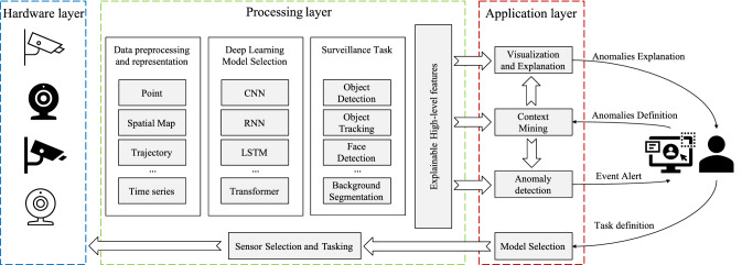
Most of the existing deep learning studies for video anomaly detection require a large volume of normal video stream training data, resulting in high model complexity and a long training time [11]. Also, the explanation process for detection is difficult since there are no semantic features that can be easily interpreted. Most of them only provide the abnormal event localization, which cannot reflect the temporal causal or the unusual human-object relationship [22]. To address these limitations, we propose an explainable and efficient deep learning framework for video anomaly detection. This framework uses pre-trained models with meaningful outputs for visualization and interpretability and captures the required features related to abnormal events. Our proposed architecture is shown in Fig. 1, where our system is divided into three layers: Hardware, processing, and application layers.
Fig. 1.
Design of the proposed deep learning framework for video anomaly detection. The hardware layer provides the raw data stream to the middle layer. The processing layer embedded with pretrained Deep Learning model generates the explainable high-level features to the application layer. In the application layer, the high-level features are visualized. It generates the contextual features based on the definition of the anomaly behavior
We consider the hardware layer as a set of distributed cameras and related drivers, which will transfer raw video streams into the system. The camera selection, position, and orientation decide the overall monitoring area and provide the associated coordination of the region of interest. For example, if the user needs to monitor the car plates, then the high-resolution camera will be selected. However, these problems of camera orientation and focus areas are not the main focus of this work. The camera operation-related tasks like camera hand-off and data fusion are handled in the processing layer. In the processing layer, the raw video data are preprocessed and made appropriate representation based on the deep learning model selection, further required by the surveillance task. The surveillance task in the processing layer may vary depending on the application layer's explanation requirement and the task definition. For example, the main focus in a supermarket is preventing shoplifting, whereas, in a train station, we may use multi-object tracking to provide crowd statistics. Then, the outputs of the selected surveillance tasks are combined and sent to the application layer for anomaly detection and explanation. The application layer provides the user interface of the surveillance system where it includes the functionalities like video visualization and camera control. The user can provide more information for the anomaly behavior based on the defined rules. For instance, in the traffic system, there must be rules that govern the movement of vehicles; for example, when the traffic light color is red, the car should stop. The rules can be implemented as relationships between traffic light colors and vehicles in the object classification task [40]. The high-level features will be fed into the anomaly detection module to generate alerts to the user whenever an abnormal event is detected. Furthermore, the sensor tasking module in the application layer receives commands from the user to control the behavior of the cameras, like turning and zooming in/out to receive more detailed information on the region of interest.
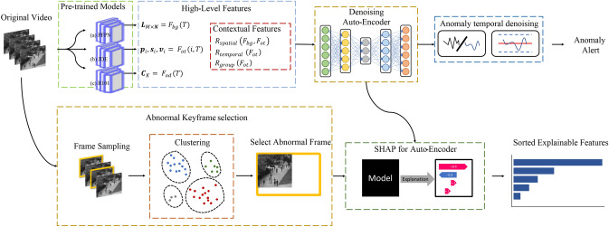
To illustrate the deep learning framework for video anomaly detection shown in Fig. 1, we select the outdoor surveillance task. Compared to the indoor surveillance task [41], the outdoor surveillance task is more complex, with more objects to be analyzed, a larger region to monitor, and more variations in the background (parking lot, avenue, playground, etc.). To address the outdoor surveillance task with the proposed deep learning framework, we present a novel explainable video anomaly detection method (summarized in Fig. 2). This method processes the contextual features (such as human location and background categories relationship) directly from the pre-trained model outputs. For our case of crowd surveillance, we choose pre-trained models for background segmentation, object tracking, and object classification. By learning features from pre-trained model output, we focus our research effort on only developing the anomaly detection method to study the individual frames, reducing the complexity of the anomaly detection model. We also propose an algorithm to explain the video anomaly detection results of abnormal behaviors and events by integrating SHAP for autoencoder [28]: (1) The proper representation of anomalies in videos. For example, a keyframe containing the most anomalous activity information can be selected as the anomaly representation. (2) Explanation of the decision-making of the anomaly detection. To address these problems, our anomaly explanation utilizes video summarization and generates interpretations of the abnormal keyframes with SHAP for autoencoder.
Fig. 2.
The architecture of the proposed explainable anomaly detection framework. In the upper part, the CNN pretrained models generate the high-level features from the video stream and feed it into the denoising autoencoder with anomaly temporal denoising. In the lower part, the video anomaly explanation consists of keyframe selection, SHAP for auto-encoder, and the sorted explainable features
Video anomaly detection
We denote a video as , where represents the video frame and . The problem of frame-level video anomaly detection can be defined as follows.
| 1 |
where denotes the prediction function and represents the prediction score of the video frame. Conventional deep learning-based video anomaly detection methods get through learning end-to-end deep model [11]. More specifically, the models use the input video frame to directly get . However, deep model training in an end-to-end fashion lacks interpretability and needs a long training time. To attain accurate, explainable, and efficient results, we extract high-level features from pre-trained models when designing . Generally, video analysis tasks need to perform image segment, object identification, and tracking. Besides, context mining is often used for video analysis. With this kind of data, we can predict and interpret a video frame comprehensively. Hence, we design a function that firstly uses pre-trained CNN models to obtain the high-level concept and context features based on background segmentation, object classification, multi-object tracking, and semantic context information, and then, uses DAE with temporal denoising process to predict the video frame base on these features. The features are also used by DAE to explain anomalies through SHAP and video summary. According to the above consideration, an explainable and efficient deep learning framework is proposed. The architecture of the proposed framework for video anomaly detection is shown in Fig. 2.
Feature extraction
There exist many possible causes of abnormal events, such as abnormal object appearance, abnormal motion, and abnormal object location. We use pre-trained models such as background segmentation, object classification, and multi-object tracking to extract the anomalies in a video. To build the background segmentation feature, we consider the Panoptic Feature Pyramid Network (PFPN) [36]. As discussed in Sect. 2, PFPN provides instance segmentation and background segmentation and has proved to be a stable solution by being wildly used as a pre-trained model on many other fields [37–39]. We run this CNN-based model on the Detectron2 platform (The Facebook AI Research software system) [42]. It provides state-of-art detection and segmentation algorithms and a large set of baseline results and pre-trained models. PFPN solves the unified task of instance segmentation and semantic segmentation (for stuff classes: amorphous background regions, e.g., rivers, wall). The model is pre-trained on the COCO train2017 dataset and validated on COCO val2017 [43]. COCO dataset is a large-scale object detection dataset and proving over 330,000 images and 1.5 million object instances. The large volume of training data provides better accuracy and generalization for the pre-trained model. This model has an inference speed of 0.067 s per image and masks average precision (AP) of 38.5 on COCO val2017 with GPU V100. The speed allows us to have near-real-time (up to 15 FPS) visualization of the background segmentation results. We only select semantic segmentation for background segmentation. The output can be written as
| 2 |
where for the input image at time , the PFPN model outputs a matrix with classified background labels as well as height and width information. Here we note that this model can be trained on different datasets to improve the segmentation result. For the video anomaly detection task, the background segmentation will only update their results when the vision content changes (e.g., the changing of the ambient light, turning the camera direction, switching the camera). We did not directly utilize the matrix output of background segmentation into the anomaly detection model. Instead, we perform a contextual feature extraction method to process the output and then convert it to a scalar output.
Considering most outdoor activities involving pedestrian movement, we use the Joint Detection and Embedding (JDE) model [44] to get the pedestrian detection and tracking feature. JDE is a variant of real-time object detection YOLOv3 (you only look once, version 3) [45] for real-time multi-object tracking. The JDE model is pre-trained on the MOT-16 training set. The model inference speed is around 38 FPS with the input frame size pixels on an Nvidia Titan Xp GPU. The output is person tracking results, which can be written as:
| 3 |
where represent the box coordinates, size (width and height), and the velocity of the person with ID . Given an image at time as the input of the multiple objects tracking model , we will obtain the above outputs for each person. The tracking feature could provide statistical information for each person (trajectories and average speed). We will use these features as the crowd activity analysis in the context mining module.
For the appearance feature, we consider the model ResNet-101 (R101) [35] implemented on the Detectron2 platform. As we mentioned in Sect. 2, ResNet is one of the most successful object detection architectures and has been integrated into many official machine learning platforms, such as TensorFlow and Pytorch. We choose ResNet as the object detection backbone of our deep learning framework by considering its extensive usage and outstanding performance. It has been pre-trained on the COCO train2017 dataset. The output includes 80 object categories. The R101 model is a CNN-based model that is 101 layers deep. The pre-trained model has an inference speed of 0.051 s per image and the box AP of 42.0 on COCO val2017 with GPU V100. The output of the R101 model is written as
| 4 |
where the output is a vector with a length equal to the output categories number . When given the frame input at time , the R101 model will produce category outputs as a vector. We directly use this vector as an input for the anomaly detection model. We note here the object classification model is crucial to the performance of the video anomaly detection since many abnormal frames are followed by the appearance of the unseen object. We choose the COCO dataset to make it the baseline for the context mining comparison.
Context mining
Even though pre-trained models provide useful features, we still need inter-relationship information between objects. Hence, we process contextual features to improve anomaly detection performance. For that, we classified the extracted contexts as spatial context, temporal context, and group context. The contextual features can reflect prior knowledge from the user who evaluates the pre-trained models' visualization results. If the visualization shows the pre-trained model result is wrong, then the related erroneous context should be adjusted or removed. For example, the user can add a weapon appearance into a blacklist to trigger an alert when a weapon shows up in the video frame. By allowing users to add self-defined contextual features, the searching space for anomaly events can be significantly reduced.
Features that capture the relative spatial relationships among persons or objects of interest are defined as spatial context. We denote the mining spatial relationship process between different pre-trained models result as . The spatial relationship including the intra-spatial relationship and the inter-spatial relationship. The intra-spatial relationship represents the inclusion result of regional classifications with height and width and the object detection/tracking results with coordinates . The inter-spatial relationship consists of the adjacent object combinations. One type of spatial anomaly is a certain type of object that is not allowed to appear in a certain type of region. For instance, “trucks are not allowed to drive on the sidewalk”. In our case, we use the following formula to represent the spatial relationship between object tracking and background segmentation:
| 5 |
where the output represents the regional relationship between types region and types of tracking objects. The denotes considering the intra-spatial relationship between models and . Some approaches learned trajectories in training data to determine feasible areas, which means that regions without moving objects will be treated as prohibited regions. For example, Zhao et al. predict car trajectory and label the moving car on the Traffic dataset [21]. This kind of mapping has two major shortages. Firstly, it needs to collect enough trajectories in training data to cover the feasible region, which is hard, especially when the monitoring area is large. Secondly, the location will degenerate when the camera position or orientation is adjusted. By using the spatial relationship between tracking objects and the background type, the above shortages will be overcome since we do not consider the absolute coordinates but the categorized relationship.
Features that capture the relative temporal relationships among the temporal attribute of persons or objects of interest are defined as temporal context. We denote the mining temporal relationship process among the pre-trained models result with timestamps as . The temporal context is widely used in the activity recognition task since the current action could imply the next action. For example, “get off the car” is likely to have “closed-door” behavior followed. In our case, we could consider the speed history of each person then update the Overspeed sign:
| 6 |
where is the frame-level Overspeed sign in the time range . denotes the relative relationship among the results of object tracking output . This feature smooths the speed measurement of the object tracking output. In frame-level anomaly detection, the object speed in each frame is not a reliable feature since many movement speeds are periodic (walking, running, riding a bicycle with changing direction, etc.). In this case, we consider the maximal average speed for each person and find the corresponding appearance in each frame.
Finally, we consider mining the group context (frame-level crowd activity statistic) from object tracking features. It includes the min, max, and median value of the coordinates, and speed. We also use the sum of residuals in the least-squares solution of coordinates and speeds to measure the crowd sparsity. When all persons move in the same direction, then the sum of residuals will equal zero since the moving direction falls into line (each residual is zero).
Anomaly detection method
For anomaly detection, we are mainly focusing on the behavior analysis of pedestrians by applying denoising autoencoder (DAE), which is a variant of the basic autoencoder (AE) [46]. DAE is trained through reconstructing a clean input by a corrupted input , where, is the noise factor, and is the noise data distribution. In a basic one-layer DAE, the forward propagation for a basic AE with one hidden layer is:
| 7 |
| 8 |
where is the vector of the hidden layer unit activities, is the reconstruction feature vector in the output layer, is an activation function, is the weight matrix between the input layer and the hidden layer, is the weight matrix between the hidden layer and output layer, and and are the offset vectors. A basic DAE is learned by minimizing the loss function . Deep DAE can be achieved by using multiple hidden layers that can learn the complicated distribution by given samples due to its multiple feature representation spaces [47]. The backpropagation algorithm [48] is used to train DAE. Our DAE uses the sigmoid activation function for each hidden layer and identity function for the output layer.
One important aspect of our version of DAE is that we use batch normalization (BN) that enables performance improvement and more stable training of DAE [49]. BN uses the mean and variance of batches of training data to perform batch normalization. As a single unit in DAE, its output is given by:
| 9 |
where is the learned weight, is the learned bias, and is the input. After applying BN, its output is given by:
| 10 |
where is a batch training data that can compute the mean and the standard deviation . In the test phase, the parameters and learned by the original model parameters are used to represent the ranges of inputs to .
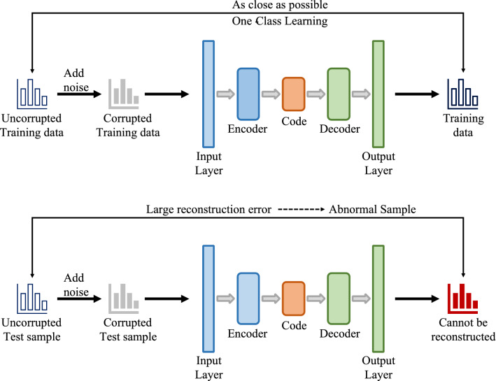
Our DAE architecture is shown in Fig. 3. The number of units in the input is determined by the input feature space. To reconstruct observations, the output layer also has the same number of nodes in the input layer. We add three fully connected hidden layers into DAE to form deep DAE. The layer nodes numbers are 50, 30, and 50, respectively (this configuration set provided the best results based on our experiments). The code layer (The middle layer with the 30 nodes) stores the compressed representation space for the input features. Gaussian distribution noise matrix is added into the input vector. Our version of DAE learns the parameters using Adam gradient-based optimization algorithm [50] with mini-batch training to minimize the mean squared error (MSE) used as the reconstruction error. After completing the training phase with denoising Gaussian noise, our DAE can detect the anomaly. An observation that belongs to normal or abnormal is determined by reconstruction error. During the test phase, an observation is normal if it has a low reconstruction error while it is abnormal if its reconstruction error is large.
Fig. 3.
The architecture of DAE for video anomaly detection
Temporal denoising
The frame-level output anomaly scores are determined by the reconstruction error between feature input and autoencoder feature output. In our pre-trained-CNN method, feature values are easily affected by the false alerts of the pre-trained model, such as the misclassification of the object detection results. The outlier value in the anomaly score curve is more likely introduced by the false alert of the pre-trained model input. To remedy this problem, we present the post-temporal denoising scheme after the autoencoder output based on the assumption that the consecutive frames have similar feature distribution.
Compared with other smoothing functions (such as Triangular filtering and average smoothing), the Savitzky–Golay filter (S-G filter) could better preserve the area, position, and width of the peak. Hence, in our temporal-denoising process, the reconstruction errors of a series of frames is filtered by the Savitzky–Golay filter [51]:
| 11 |
where is the normalizing factor, is the convolution coefficient determined by the polynomial degree, is the window size. Note here the window size and the polynomial degree of the S-G filter are decided by the pre-trained model accuracy. If the false-alert rate of the pre-trained model is higher, the required smoothness decided by and can be increased accordingly.
Video anomaly explanation
To increase the interpretability of our video anomaly detection method, we propose a video anomaly explanation method by using SHAP (see the lower part of Fig. 2). We first introduce the background of our method, including SHAP, and using SHAP to explain the autoencoder. Then, we demonstrate how our method integrates SHAP and autoencoder to explain the anomaly detection results.
SHAP (SHapely Additive exPlanations)
With the rapid growth of deep learning research, the accuracy of the method has been significantly improved. However, there is also an urgent need for a more transparent model to explain the model decision-making. In some applications that emphasize interpretability, researchers prefer to use a simple model like the linear model to predict even its accuracy is lower than other complex models. For explaining the prediction results of black-box models, many methods have been proposed to interpret the model output, such as DeepLIFT [52] and LIME [53]. To generalize those related methods, Lundberg and Lee propose SHAP (SHapely Additive exPlanations) as a unified approach to interpret model prediction [13].
An explanation model can be expressed as:
| 12 |
where is the simplified binary input vector with length and value 0 or 1. The original input can be mapped from the simplified input and . Once we found the result of the explanation model, the weight explains the importance of the input feature . can be calculated from game theory results, where the is known as Shapely value.
The weighting kernel can be used to approximate the Shapely value [13], which are given by:
| 13 |
where is the length of non-zero elements. The loss function for optimization is defined as:
| 14 |
By minimizing the loss function over the training dataset , the approximation of Shapely value can be calculated:
| 15 |
where is the penalty term of complexity.
Using SHAP to explain autoencoder
Autoencoder has been widely used on anomaly detection tasks [54]. However, there is little research on explaining the results of the autoencoder. Based on the model-agnostic explanation method kernel SHAP, Antwarg et al. propose a method to explain the anomalies detected by autoencoder [28]. The main procedure of using SHAP to explain the autoencoder are summarized as follows:
Given the trained autoencoder and input instance, the features with top reconstruction errors are selected as the target output features.
For each selected high error feature, fit the SHAP explainer with training background set, then use SHAP explainer to attribute the input features for predicting these high error features. In this step, the target function for SHAP to approximate is the selected feature element in the autoencoder output.
The input features can be classified as contributing and offsetting features based on whether the reconstruction error is negative and positive. The contributing feature means this feature pushes the predicting value away from the true value, while the offsetting feature pushes predicting the value towards the true value.
This method inspired us to design and implement an explainable autoencoder for video anomaly detection.
The proposed method for video anomaly explanation
We propose a novel method for explaining video anomaly detection. Our method first uses a video summary to find the representative frames in a video with anomalies, then explains the autoencoder output of the keyframes using SHAP. The output is the sorted features by the importance of contributing to the anomalies in the video, which explains the video anomaly detection decision-making process.
The algorithm calculates the explainable video features using pre-trained models and trained denoising autoencoder to process the raw video frames (see Algorithm 1). Usually, consecutive frames are similar; thus, in practice, to reduce the complexity, it is widely accepted to remove the consecutive frames when they have the minimum amount of difference. Hence the first step of Algorithm 1 is to uniform sample the input video in a fixed interval to eliminate the redundant frames. In video summary, the algorithm still can summarize the major information of the video even the FPS is lowered to 5 [55]. Next, we get the feature set from the sampled frames using the pre-trained models. Then, the feature set is clustered by a K-means algorithm [56]. The nearest frame to the cluster center is the representative frame. Finally, the frames are filtered with the autoencoder anomaly scores since we focus on explaining the anomalies. We then explain the filtered output keyframes.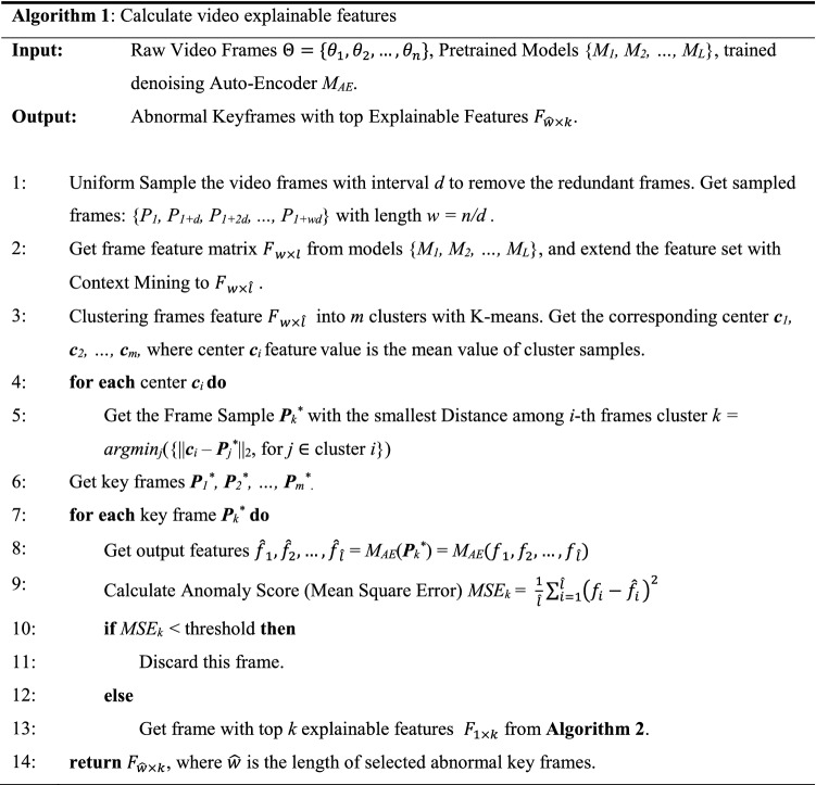
Once we find the keyframes that we are interested in, we use Algorithm 2 to get the most important features for each frame contributing to the anomalies. Algorithm 2 requires the input frame features, trained autoencoder, and the background set. The background set is part of the samples that represent the dataset for training the SHAP model. In our case, it consisted of the samples of the high-level and contextual features. The reconstruction errors are first calculated by comparing the distance between autoencoder input and output. Then we get the top error features by sorting the reconstruction errors. The features with a high error are considered as the significant factor in deciding whether the instance is abnormal. For each high error feature, we treat the autoencoder as a multi-input–single-output function to use SHAP to explain the prediction concerning the certain input instance. Depending on the positiveness of the reconstruction error, the related features of the high error feature can be classified into contributing features and offsetting features.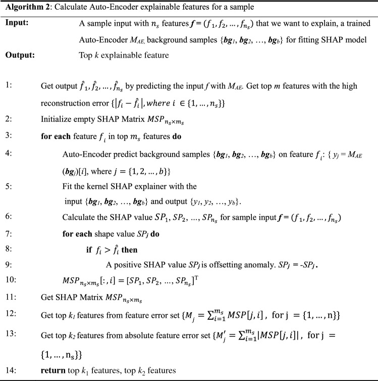
We sorted the feature by two different methods: the mean of SHAP value and the mean of absolute SHAP value. Intuitively, the sum of the SHAP value should indicate the importance of a certain feature contributing to the anomaly decision. However, many factors can affect the accuracy of the explainable model (such as the background set selection, the selection of the number of error features, etc.). Some major features have a small mean of SHAP values because the contributing value and offsetting value from different error features are neutralized. So we consider the feature importance from the sorted order of the mean of SHAP value and the mean of absolute SHAP value.
Finally, the important features of each key abnormal frame are summarized as the explanation of the anomalies in a video. We present the workflow of video anomaly explanation in Fig. 4. In shorts, our proposed method can be summarized as follows. First, select keyframes by uniform sampling the raw video and clustering the rest frames by high-level features. Then, select anomalous keyframe by the anomaly score and explain the keyframe with SHAP for the autoencoder method. Finally, sort the most important features by SHAP value, and use them to explain the anomalous event in the video.
Fig. 4.
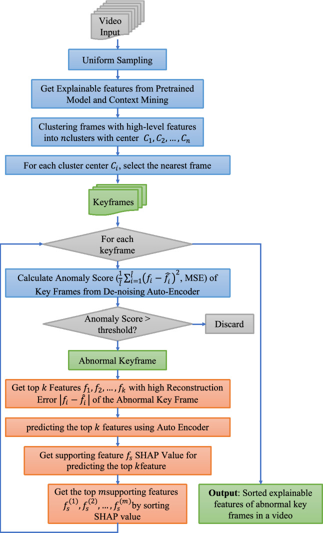
The workflow of video anomaly explanation
Experimental results and evaluation
Dataset
One of the most common outdoor activities is the movement of pedestrians. To evaluate our proposed method for outdoor activities surveillance, we show the anomaly detection result on the UCSD Ped1 and Ped 2 datasets [6]. The UCSD datasets provide video of people on pedestrian walkways at the University of California San Diego. As a popular video anomaly detection public dataset, it has been wildly used as the evaluation of video anomaly detection algorithm. The Ped1 dataset has 34 training videos and 36 testing videos. Each video consists of 200 frames with pixels at 30 FPS. The Ped2 dataset has 16 training videos and 12 testing videos. The video frame number of the Ped2 dataset ranges from 120 to 180 frames with pixels. The training video only includes pedestrians. Both Ped1 and Ped2 provide completed frame-level abnormal labels and partial pixel-level abnormal labels. In this experiment, we only consider the frame-level samples since our work mainly considering the contextual features. The abnormal event includes unexpected entities (bicycle, skateboard, motorcycle, etc.), irregular trajectory (deviate from the major moving direction), and entering the prohibitive region (walking on the grass).
Experiment Setup
We get high-level features from the pre-trained models. The details are demonstrated in Sect. 3. The inference of the pre-trained model is running on the Google Colaboratory [57] server.
The DAE is implemented on Tensorflow and Keras. We use the Adam optimizer and the MSE loss function to optimize the model. The epoch of training for Ped1 and Ped2 was set to 25 and 28, respectively. The batch size was set to 120. In the experiments, we set the noise factor as {0.01, 0.05, 0.1, 0.15, 0.2, 0.25, 0.3, 0.35, 0.4} and choose the better result. The training and test evaluation of the anomaly detection models are running on a computer with the 64-bit Windows 10 Operating System and equipped with 16 GB DDR4 RAM and an Intel Core i7-9750H CPU running at 2.60 GHz.
Visualization
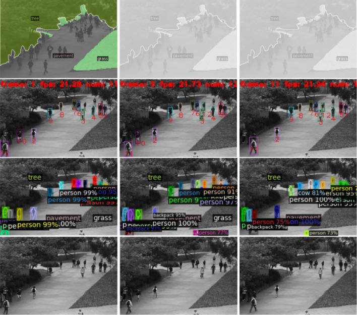
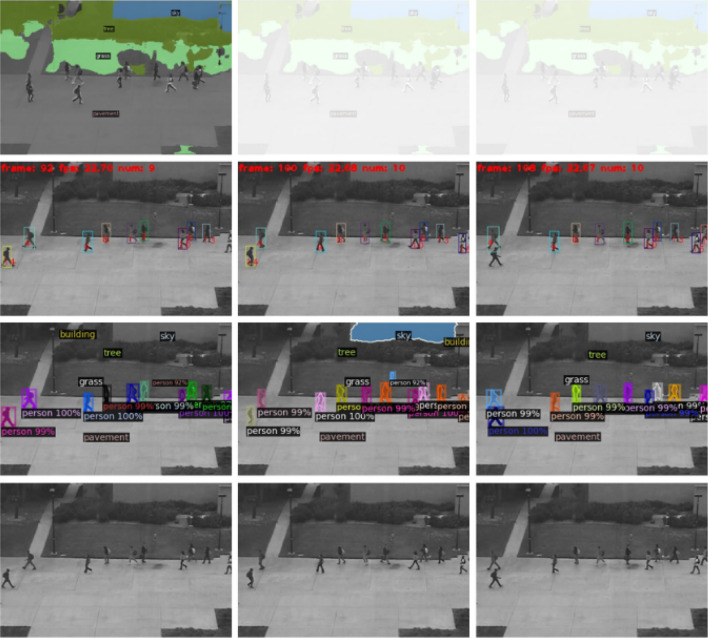
To understand the outputs of context mining, we visualize the results of the embedded computer vision task on both datasets. Figures 5 and 6 present examples of the visualization results on both training datasets. For each figure, the images in the first row show the background segmentation results. In the implementation, the user is supposed to select the frames with clear segmentations since their segmentation results are not affected by the ambient light. Only when the camera position is adjusted, the background segmentation should be updated. The images in the second row show the multiple object tracking results. The model assigns a unique ID to each pedestrian. By calculating the difference between the frames, we can get the movement of each person. In the images of the third row, we present the object classification result used as baseline features of our video anomaly detection model, and the accuracy determines the lower bound of our model performance since most anomaly event comes from the occurrence of abnormal objects. When the embedded pre-trained model results are visualized, the user can evaluate the quality of the outputs and decide the principle of formulating contextual features. For instance, if the background segmentation results are unqualified (obvious boundary mismatch or misclassification in pre-trained model evaluation), we should not consider the relative position context as the anomaly detection feature. In our case, we keep all the pre-trained model outputs to generate the contextual features on the Ped1 dataset and we discard the background segmentation results in the Ped2 dataset since the visualization shows that most of the background segmentation results are unsatisfactory. Since we removed the background segmentation, the relevant mined spatial contexts are also removed from the features. In Ped1, the dimension of input features is 100 while in Ped 2 it is 81 since we remove the unreliable features by checking the visualization results.
Fig. 5.
Visualization of the embedded task result from Ped1 training dataset. From 1st to 4th row is the background segmentation, pedestrian tracking, object classification, origin frames, respectively. Note: the first row is using the same image since the background segmentation should keep constant when the camera is fixed
Fig. 6.
Visualization of the embedded task result from the Ped2 training dataset. From 1st to 4th row is the background segmentation, pedestrian tracking, object classification, origin frames, respectively. The first row uses the selective fixed results
Results
We evaluate the performance of our video anomaly detection method by considering the effect of the contextual features and training data volume. Receiver Operative Characteristic curve (ROC curve), Area Under the ROC curve (AUC), and Equal Error Rate (EER) are the used metrics since they are widely used metrics for the UCSD Ped1 and UCSD Ped2 datasets [6, 58]. To study the effectiveness of our approach, we compare it with state-of-the-art approaches. The ROC curve results are shown in Figs. 7 and 8. The AUC and EER results are summarized in Table 1. Here we use the bold text to highlight the state-of-the-art performance.
Fig. 7.
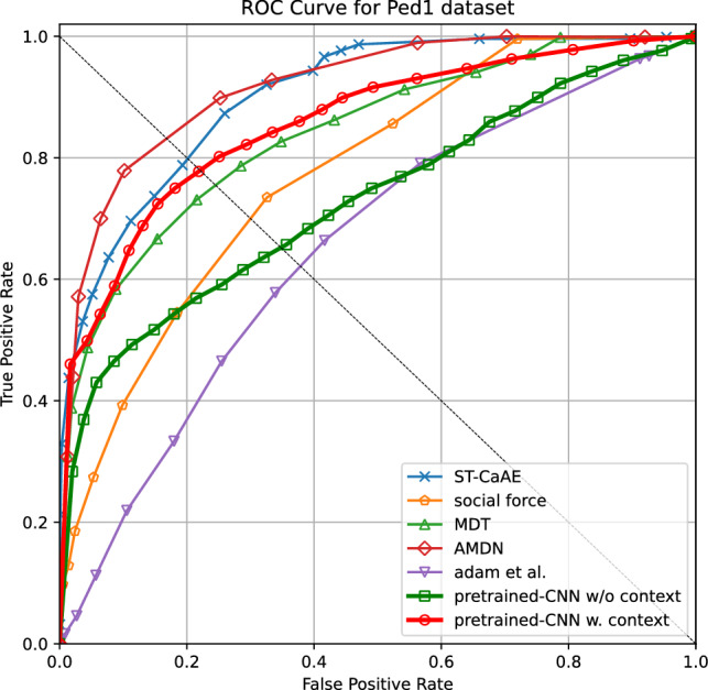
ROC curve of Ped1 dataset
Fig. 8.
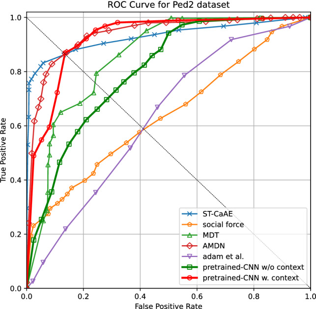
ROC curve of Ped2 dataset
Table 1.
Frame-level performance comparison of the anomaly event detection
| Methods | Ped1 [6] | Ped2 [6] | ||
|---|---|---|---|---|
| AUC (%) | EER (%) | AUC (%) | EER (%) | |
| Adam [6] | 65.0 | 38.0 | 63.0 | 42.0 |
| Social force [16] | 67.5 | 31.0 | 63.0 | 42.0 |
| MDT [6] | 81.8 | 25.0 | 82.9 | 25.0 |
| Compact feature set [17] | 82.0 | 21.1 | 84.0 | 19.2 |
| Convex polytope ensemble [59] | 78.2 | 24.0 | 80.7 | 19.0 |
| RBM [60] | 70.3 | 35.4 | 86.4 | 16.5 |
| ST-AE [58] | 89.9 | 12.5 | 87.4 | 12.0 |
| ConvAE [11] | 81.0 | 27.9 | 90.0 | 21.7 |
| ConvLSTM-AE [12] | 75.5 | N/A | 88.1 | N/A |
| Two-Stream R-ConvVAE [4] | 75.0 | 32.4 | 91.7 | 15.5 |
| AMDN [3] | 92.1 | 16.0 | 90.8 | 17.0 |
| STAN [5] | 82.1 | N/A | 96.5 | N/A |
| ST-CaAE [18] | 90.5 | 18.8 | 92.9 | 12.7 |
| Optical flow-GAN [19] | 97.4 | 8 | 93.5 | 14 |
| Our preliminary work [67] | 84.1 | 23.8 | 92.4 | 14.9 |
| Our method | 85.9 | 22.0 | 92.4 | 13.5 |
| Our method without Context | 73.1 | 34.8 | 80.1 | 29.3 |
For the method without contextual features, we only keep the appearance feature (for more information, refer to the approach in [31]). The result shows that the contextual feature effectively integrates the information of movement and semantic result and improves the performance of the anomaly detection method. Without contextual feature, the AUC of our approach is 73.1% and 80.1% in the UCSD Ped1 dataset and the UCSD Ped2 dataset, respectively. Our approach with contextual feature has achieved the AUC of 85.9% and 92.4% in the UCSD Ped1 dataset and the UCSD Ped2 dataset.
As shown in Table 1, our model outperforms the approaches with low model complexity (MDT [6], Adam [6], Social force [16], Compact feature set [17], convex polytope ensemble [59], and RBM [60]) and several approaches with large model complexities by adding convolutional layers (ConvAE [11], ConvLSTM-AE [12], Two-Stream R-ConvVAE [4]), and can achieve comparable performance compared to ST-AE [58], and AMDN [3]. Our method achieves 92.4% AUC on the Ped2 data set and 85.9% AUC on the Ped1 dataset. Hence, the DAE with relatively low model complexity can achieve comparable results using the features derived from the pre-trained deep models. Our model without contextual features achieves 80.1% AUC in Ped2 while 73.1% on Ped1, which means an accurate pre-trained model will improve our final model performance. Most of the competing methods in this study trained the large model while we only consider using the high-level and contextual features derived from pre-trained models to reduce the model complexity for the anomaly detection model. For example, in the Ped1 dataset, the ConvAE model uses the fully convolutional autoencoder [11]. It has 6 convolutional layers and 4 pooling layers in the encoder and decoder. The input layer dimension is . The training process requires up to 16,000 epochs to converge. ConvLSTM-AE model adds 10 convolutional long short-term memory layers that are interconnected in addition to the convolutional layers [12]. The training process requires up to 60,000 epochs. In our case, we only use 3 fully connected layers with an input dimension of 100 and the training process only requires up to 25 epochs to converge in the Ped1 dataset and 200 epochs in the Ped2 dataset with an input dimension of 81. We also list the state-of-the-art approaches (STAN [5], ST-CaAE [18], and Optical flow-GAN [19]). In addition to training CNN to learn the spatial features, STAN and Optical flow-GAN takes the Generative Adversarial Network architecture to improve the performance. However, it increases the model complexity. For example, STAN has 17 convolutional layers with kernel size between and where the number of layers has almost tripled compared to ConvAE. ST-CaAE consists of adversarial network ST-AAE and convolutional network ST-CAE. ST-AAE has four 3D convolutional layers and the corresponding four 3D deconvolutional layers, while ST-CAE has three 3D convolutional layers and three 3D deconvolutional layers. Each convolution layer uses kernels with the size , and the number of kernels is 16 in the input convolutional layer. The ST-CaAE also needs to be trained on appearance stream and motion stream, respectively, which further increases the model complexity. Compared to the above models, our approach extracts the complicated part into pre-trained models and only needs to train the decision model with the fully connected layers.
Our model also shows the advantages of the interpretability of abnormal event decisions. The other models such as Two-Stream R-ConvVAE use the reconstruction error on each pixel to locate the anomaly region [4]. This method only reflects the spatial features of decision-making and cannot explain the temporal or group anomalies. Since our input features are high-level features and semantically meaningful features, we can directly show the reconstruction error vector to explain the decision-making process. Note that here we just use three pre-trained deep models to extract features, and we have shown in the experiments that they are already beneficial. It is expectable that more profit can be attained by using more pre-trained models that can be used to derive varied features. We leave the possibilities for future exploration.
Time analysis
We compare our method running time with several algorithms, as shown in Table 2. It reports the average running time of each frame during the test phase. Our method is significantly faster than MDT [6], AMDN [3], Xu et al.’s method without GPU [61], and Hierarchical framework [62]. Our method is also faster than ST-CNN [63], AED [64], and ICN [65]. Compared to the state-of-the-art method like XU et al. method with GPU and Two-Stream R-ConvVAE [4], our method achieves comparable run time speed. Note that the GPU is only used on the pre-trained models for getting the high-level features in our approach. We calculate the pre-trained models running time by taking the maximum value of inference time per frame from PFPN, JDE, and R101 since these pre-trained models can run simultaneously by their corresponding GPU described in Sect. 3.2.1, which is . The pre-trained model inference speed can be improved by the advance of computer vision research and the improvement of GPU technologies. Our lightweight denoising autoencoder does not need GPU, and the average inference time for each frame is on the UCSD Ped1 dataset and on the UCSD Ped2 dataset.
Table 2.
Frame-level anomaly detection running time comparison
| Method | Platform | CPU | GPU | Running time (seconds per frame) | |
|---|---|---|---|---|---|
| UCSD Ped1 | UCSD Ped2 | ||||
| MDT [6] | – | 3.0 GHz | – | 25 | – |
| AMDN [3] | MATLAB | 2.1 GHz | Nvidia Quadro K4000 | 5.2 | 7.5 |
| XU et al. [61] without GPU | Pytorch | 2.1 GHz | – | 2.68 | 6.84 |
| Hierarchical framework [62] | MATLAB | 3.0 GHz | – | 5 | 5 |
| ST-CNN [63] | Caffe | 2.8 GHz | – | 0.37 | 0.39 |
| AED [64] | N/A | N/A | N/A | 0.073 | – |
| ICN [65] | Tensorflow | 2.4 GHz | NVIDIA Tesla K40c | – | 0.18 |
| XU et al. [61] with GPU | Pytorch | 2.1 GHz | Nvidia TITAN X | 0.00242 | 0.00265 |
| Two-Stream R-ConvVAE [4] | Tensorflow | 2.6 GHz | Nvidia TITAN X | 0.0012 | – |
| Oursa | Tensorflow | 2.6 GHz | Nvidia V100, Nvidia TITAN Xp |
|
|
aOur pre-trained model running time
We also show the training time comparison among algorithms, as shown in Table 3. Since our method relies on the pre-trained model features, a large amount of training time can be saved. We only need to focus on the training of the lightweight denoising autoencoder. We take the mean value of the 10 repetitive measurements and our method only requires and for the Ped1, Ped2, and Avenue dataset (here Avenue dataset only be used for training time analysis, the epoch is set as 28), which is significantly faster than AMDN, ConvAE, TSC, and sRNNAE [66].
Table 3.
Training time comparison
| Method | Platform | CPU | GPU | Training time | ||
|---|---|---|---|---|---|---|
| UCSD Ped1 | UCSD Ped2 | Avenue | ||||
| AMDN [3] | MATLAB | 2.1 GHz | Nvidia Quadro K4000 | 9 h | 4 h | 3.5 h |
| ConvAE [11] | Caffe | Unkonwn | NVIDIA Tesla K80 | Total around 1 h 50 min | ||
| TSC [66] | TensorFlow | Unkonwn | Unkonwn | – | – | 30 h |
| sRNNAE [66] | TensorFlow | Unkonwn | Unkonwn | – | – | 1.2 h |
| Oursa | Tensorflow | 2.6 GHz | – | 5 s | 2.9 s | 9.6 s |
aSince we use pre-trained CNN model, we did not use GPU
Explanation of video anomalies
The experiment results of the video anomaly explanation method are discussed. We demonstrate our method by displaying three cases from the USCD Pedestrian dataset. We set the upper limit of the number of keyframes as 3 and the number of top important features as 6. It is worthwhile to mention that the number of keyframes is a hyperparameter, and the value varies by the setting of video, such as the video length, event number, etc. As described in Algorithm 2, we skip the keyframe without abnormal events since we are only interested in explaining anomaly.
Sample case 1: Ped1 video Test017
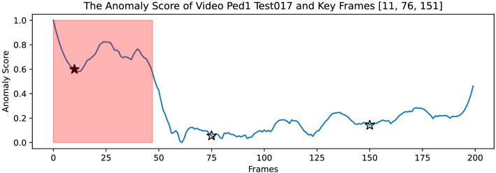
The video summary result of video Ped1_Test017 is shown in Fig. 9. In this video, there is one anomaly that occurred. The video summary presents three keyframes: frames 11, 76, and 151, where frames 76 and frame 151 are discarded because of the lower anomaly score. The remaining keyframes 11 summarize the major activities on video Ped1_Test017.
Fig. 9.
The anomaly score of video Ped1_Test017, the unfilled start marker is the discarded frame. The read shadow interval represents the ground truth abnormal interval
The ground truth of anomaly in this video consists of a person riding a bicycle on the pavement, as presented in Fig. 10. Here Fig. 11 shows the explanation result of frame 11 for demonstration.
Fig. 10.

The ground truth of anomalies in video Ped1_Test017 frame 11
Fig. 11.
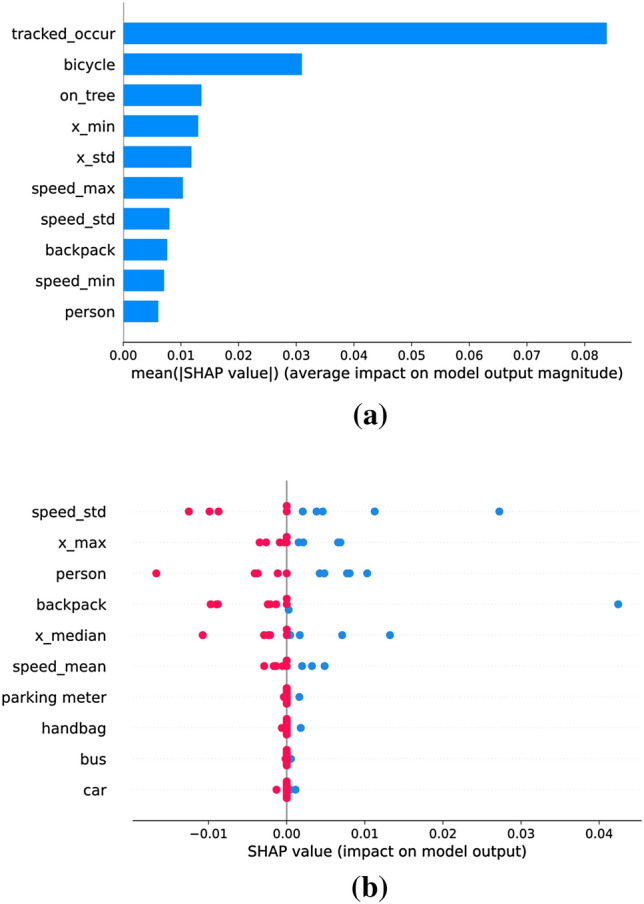
Explainable features of video Ped1_Test017 frame 76. a The important features sorted by the mean of absolute SHAP value. b The important features sorted by the mean of SHAP value
We select top 3 most important features from Fig. 11a and b to explain the frame. Therefore, frame 11 can be explained by the important features, including “tracked_occur”, “bicycle”, “on_tree”, “speed_std”, “x_max”, and “person”. Obviously, “bicycle” matches the ground truth description. In addition, other output features also assist the anomalies decision-making. For example, “tracked_occur” means some people are moving much faster in a period and are tracked automatically; this feature is highly positively related to “bicycle” and “skateboard”. The features of “person” and “on_tree” show how many people on this frame and how many people are walking near the tree. The feature, “speed_std” means the speed standard deviation of the moving objects in this frame. It implies this scenario has an abnormal event since the moving object (such as skateboarder, bicycle, and motorcycle) is faster than the walking person.
Sample case 2: Ped2 video Test004
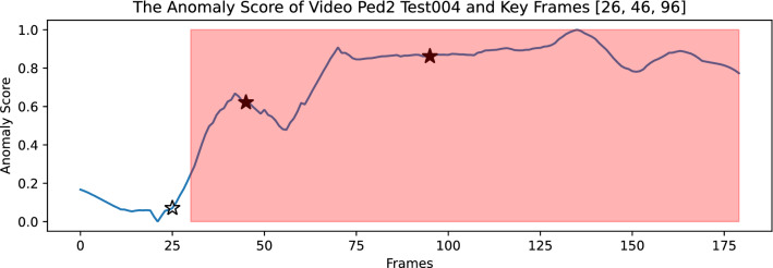
The video summary result of video Ped2_test004 yields three keyframes: frames 26, 46, and 96, as shown in Fig. 12. Frame 26 is discarded since it represents the normal case. The abnormal keyframes are correctly fallen into the ground truth abnormal interval and can represent the major activities of video anomaly in video Ped2_test004. Here we discuss the explanation results of Frame 46.
Fig. 12.
The anomaly score of video Ped2_Test004, the unfilled start marker is the discarded frame. The read shadow interval represents the ground truth abnormal interval
The Fig. 13. shows the ground truth content of frame 46, which is the abnormal keyframe of video Ped2_Test004: A car occurs on the right side of the pavement. Both sorted graph results explain this frame, as shown Fig. 14. In this case, the sorted mean absolute SHAP value features in Fig. 14a and the sorted mean SHAP value features in Fig. 14b have the same top 3 features, including “car”, “bicycle”, and “peed_min”. The feature “car” correctly reflects the ground truth of the anomaly of frame 46. However, the feature “bicycle” is a false alert since frame 46 does not include a bicycle. The feature “speed_min” is the minimum speed of all objects in the frame. In this frame, “car” feature is rank 1st in both Fig. 14a and b, which increase the confidence of the decision to make the “car” features as the anomalies.
Fig. 13.
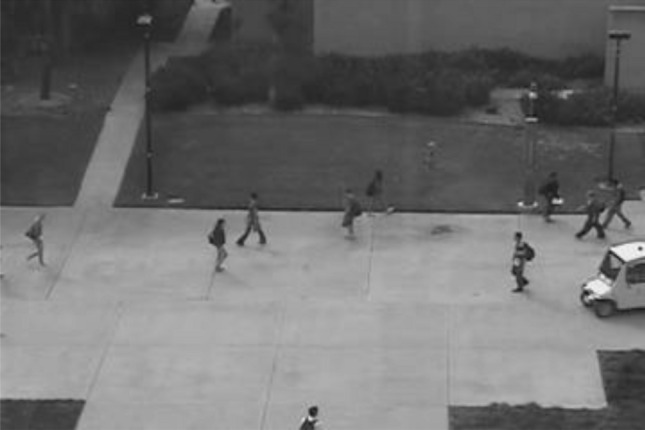
The ground truth of anomalies in video Ped2_Test004 frame 46
Fig. 14.
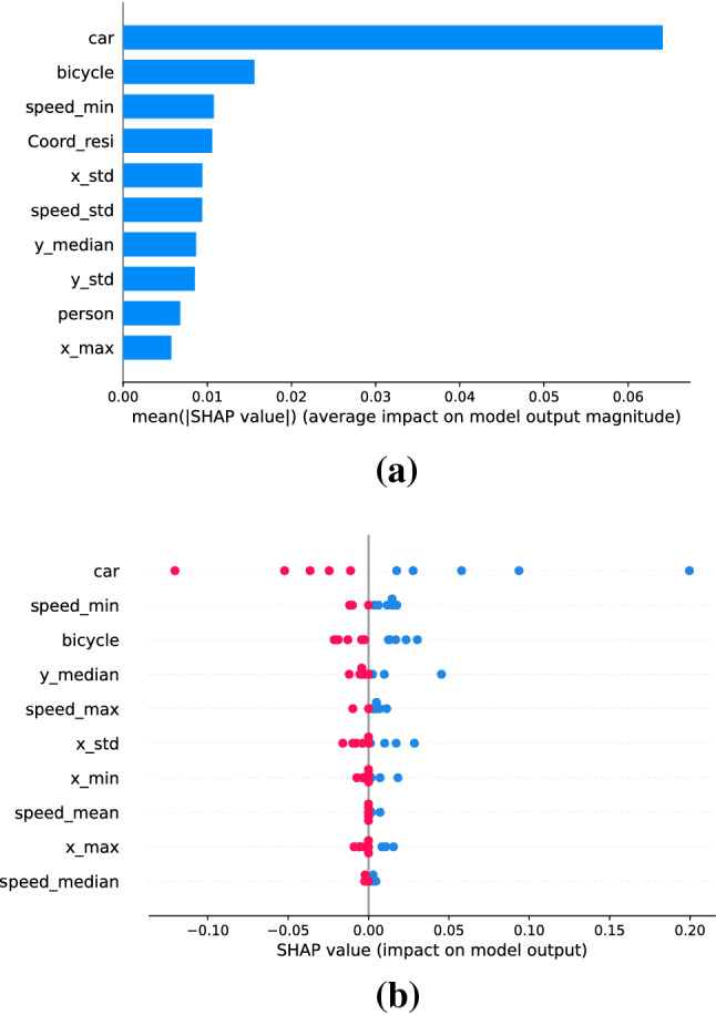
Explainable features of video Ped2_Test004 frame 46. a The important features sorted by the mean of absolute SHAP value. b The important features sorted by the mean of SHAP value
Sample case 3: Ped2_Test005
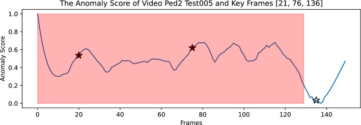
The video summary result of video Ped2_Test005 consists of three keyframes: frame 21, frame 76, and frame 136, as shown in Fig. 15. It covers the major normal and abnormal events in the video. Similarly, frame 136 will be skipped during the explanation process because of the low anomaly score. Here we present the anomaly explanation results of frame 76.
Fig. 15.
The anomaly score of video Ped2_Test005, the unfilled start marker is the discarded frame. The read shadow interval represents the ground truth abnormal interval
The ground truth content consists of a person riding a bicycle from right to left, as presented in Fig. 16. The pre-trained object detection model successfully detected the bicycle. Figure 17a shows the “bicycle” is one of the most contributing features to the anomaly detection result of frame 76. Other features like “speed_min”, “speed_mean”, and “speed_max” also support the possible occurrence of the moving object from a contextual perspective.
Fig. 16.
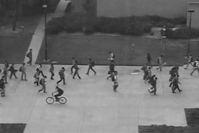
The ground truth of anomalies in video Ped2_Test005 frame 76
Fig. 17.
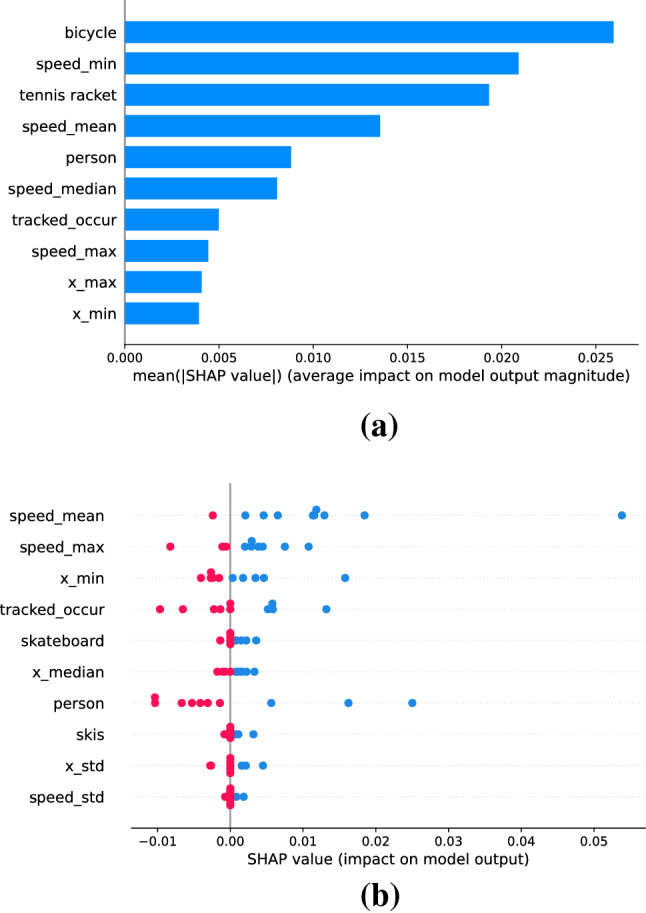
Explainable features of video Ped2_Test005 frame 76. a The important features sorted by the mean of absolute SHAP value. b The important features sorted by the mean of SHAP value
Conclusion
This work presents a novel design of an explainable and efficient video anomaly detection framework based on the high-level features from the pre-trained models and using a denoising autoencoder to detect anomalous video events and provide anomaly explanations. Our method selects three pre-trained models (background segmentation, object classification, and object tracking) to get the appearance feature and Spatio-temporal feature. The UCSD pedestrian datasets are used to evaluate our approach and to compare it with several state-of-the-art methods. Our experimental results show that contextual features improve model performance and interpretability. Moreover, our proposed model achieves comparable results and provides more accurate anomalies explanation with low model complexity, short training time, and low computational overhead. Our approach is not developed to replace state-of-the-art approaches; instead, it offers a better understanding of how pre-trained deep learning models can be used for video anomaly detection, especially when a large volume of training data is unavailable for complex models. Our method can also increase model interpretability, which is crucial to modern machine learning. In addition, the run time analysis shows our method is significantly efficient in the training process.
Acknowledgements
This work is partly supported by the Air Force Office of Scientific Research (AFOSR) Dynamic Data-Driven Application Systems (DDDAS) award number FA9550-18-1-0427, National Science Foundation (NSF) research projects NSF-1624668 and NSF-1849113, (NSF) DUE-1303362 (Scholarship-for-Service), National Institute of Standards and Technology (NIST) 70NANB18H263, and Department of Energy/National Nuclear Security Administration under Award Number(s) DE-NA0003946.
Biographies
Chongke Wu
is a graduate student in the Electrical and Computer Engineering Department at the University of Arizona. He’s a research assistant in the Autonomic Computing Laboratory. His research interest includes cybersecurity and machine learning. Chongke Wu has a MS in Control Science and Engineering from Beihang University.
Sicong Shao
received the M.Sc degree in Electrical Engineering from State University of New York at Binghamton, Binghamton, NY, USA, and the Ph.D. degree in Electrical and Computer Engineering from The University of Arizona, Tucson, AZ, USA. His research interest includes machine learning, cybersecurity, data mining, natural language processing, and social media analysis.
Cihan Tunc
is an assistant professor in the Computer Science & Engineering at University of North Texas (UNT). His research interests include cybersecurity, cloud computing, Internet of Things (IoT), and social media analysis for cybersecurity. Cihan Tunc has a PhD from the Electrical and Computer Engineering Department at the University of Arizona.
Pratik Satam
received the B.E. degree in electronics and telecommunication engineering from the University of Mumbai, in 2013, and the M.S. and Ph.D. degrees in electrical and computer engineering from The University of Arizona, Tucson, AZ, USA, in 2015 and 2019, respectively. Since 2019, he has been a Research Assistant Professor with the Department of Electrical and Computer Engineering, The University of Arizona. His current research interests mainly include autonomic computing, cyber security, cyber resilience, secure critical infrastructures, and cloud security.
Salim Hariri
(Senior Member, IEEE) received the M.Sc. degree from The Ohio State University, Columbus, OH, USA, in 1982, and the Ph.D. degree in computer engineering from the University of Southern California, in 1986. He is currently a Full Professor and The University of Arizona site Director of the NSF-Funded Center for Cloud and Autonomic Computing. He founded the IEEE/ACM International Symposium on High Performance Distributed Computing (HPDC). He is also the co-founder of the IEEE/ACM International Conference on Cloud and Autonomic Computing. He has coauthored three books on autonomic computing, parallel, and distributed computing, and edited Active Middle- ware Services, a collection of articles from the second annual AMS Workshop published by Kluwer, in 2000. He serves as the Editor-in-Chief of the scienti_c journal Cluster Computing, which presents research and applications in parallel processing, distributed computing systems, and computer networks.
Footnotes
Publisher's Note
Springer Nature remains neutral with regard to jurisdictional claims in published maps and institutional affiliations.
Contributor Information
Chongke Wu, chongkewu@email.arizona.edu.
Sicong Shao, sicongshao@email.arizona.edu.
Cihan Tunc, Email: cihan.tunc@unt.edu.
Pratik Satam, pratiksatam@email.arizona.edu.
Salim Hariri, Email: hariri@ece.arizona.edu.
References
- 1.Vigne, N.G.L., Lowry, S.S., Markman, J.A., Dwyer, A.M.: Evaluating the use of public surveillance cameras for crime control and prevention. US Department of Justice, Office of Community Oriented Policing Services. Urban Institute, Justice Policy Center, Washington, DC (2011)
- 2.Lin, L., Purnell, N.: A world with a billion cameras watching you is just around the corner. Wall Str. J. (2019)
- 3.Xu, D., Ricci, E., Yan, Y., Song, J., Sebe, N.: Learning deep representations of appearance and motion for anomalous event detection. In: Procedings of the British machine vision conference 2015, pp. 8.1–8.12 (2015)
- 4.Yan S, Smith JS, Lu W, Zhang B. Abnormal event detection from videos using a two-stream recurrent variational autoencoder. IEEE Trans. Cogn. Dev. Syst. 2020;12(1):30–42. doi: 10.1109/TCDS.2018.2883368. [DOI] [Google Scholar]
- 5.Lee, S., Kim, H. G., Ro, Y. M.: STAN: spatio-temporal adversarial networks for abnormal event detection. In: 2018 IEEE international conference on acoustics, speech and signal processing (ICASSP), pp. 1323–1327 (2018)
- 6.Mahadevan, V., Li, W., Bhalodia, V., Vasconcelos, N.: Anomaly detection in crowded scenes. In: 2010 IEEE computer society conference on computer vision and pattern recognition (2010)
- 7.Kim, J., Grauman, K.: Observe locally, infer globally: a space-time MRF for detecting abnormal activities with incremental updates. In: 2009 IEEE Conference on Computer Vision and Pattern Recognition (2009)
- 8.Lu C., Shi, J., Jia, J.: Abnormal event detection at 150 FPS in MATLAB. In: 2013 IEEE International Conference on Computer Vision (2013)
- 9.Xu, H., Gao,Y., Yu, F., Darrell, T.: End-to-end learning of driving models from large-scale video datasets. In: 2017 IEEE Conference on Computer Vision and Pattern Recognition (CVPR) (2017)
- 10.Shao S, Tunc C, Al-Shawi A, Hariri S. An ensemble of ensembles approach to author attribution for internet relay chat forensics. ACM Trans. Manag. Inf. Syst. 2020;11(4):1–25. doi: 10.1145/3409455. [DOI] [Google Scholar]
- 11.Hasan, M., Choi, J., Neumann, J., Roy-Chowdhury, A.K., Davis, L. S.: Learning temporal regularity in video sequences. In: 2016 IEEE Conference on Computer Vision and Pattern Recognition (CVPR) (2016)
- 12.Luo, W., Liu, W., Gao, S.: Remembering history with convolutional LSTM for anomaly detection. In: 2017 IEEE International Conference on Multimedia and Expo (ICME) (2017)
- 13.Lundberg, S.M., Lee, S.: A unified approach to interpreting model predictions. In: Proceedings of the 31st International Conference on Neural Information Processing Systems, pp. 4768–4777 (2017)
- 14.Zhu Y, Nayak NM, Roy-Chowdhury AK. Context-aware activity recognition and anomaly detection in video. IEEE J. Sel. Top. Signal Process. 2013;7(1):91–101. doi: 10.1109/JSTSP.2012.2234722. [DOI] [Google Scholar]
- 15.Adam A, Rivlin E, Shimshoni I, Reinitz D. Robust real-time unusual event detection using multiple fixed-location monitors. IEEE Trans. Pattern Anal. Mach. Intell. 2008;30(3):555–560. doi: 10.1109/TPAMI.2007.70825. [DOI] [PubMed] [Google Scholar]
- 16.Mehran, R., Oyama, A., Shah, M.: Abnormal crowd behavior detection using social force model. In: IEEE Conference on Computer Vision and Pattern Recognition (CVPR), 2009, pp. 935–942 (2009)
- 17.Leyva R, Sanchez V, Li C-T. Video anomaly detection with compact feature sets for online performance. IEEE Trans. Image Process. 2017;26(7):3463–3478. doi: 10.1109/TIP.2017.2695105. [DOI] [PubMed] [Google Scholar]
- 18.Li, N., Chang, F., Liu, C.: Spatial-temporal cascade autoencoder for video anomaly detection in crowded scenes. IEEE Trans. Multimed. pp. 1–1 (2020)
- 19.Ravanbakhsh, M., Nabi, M., Sangineto, E., Marcenaro, L., Regazzoni, C., Sebe, N.: Abnormal event detection in videos using generative adversarial nets. In: 2017 IEEE international conference on image processing (ICIP), pp. 1577–1581 (2017)
- 20.Hikvision.com, 2020. [Online]. https://www.hikvision.com/content/dam/hikvision/en/brochures-download/vertical-solution-brochure/Safe-City-Solution-Brochure.pdf.
- 21.Zhao, Y., Deng, B., Shen, C., Liu, Y., Lu, H., Hua, X.S.: Spatio-temporal autoencoder for video anomaly detection. In: Proceedings of the 25th ACM International Conference on Multimedia, pp. 1933–1941 (2017)
- 22.Nguyen, T.N., Meunier, J.: Anomaly detection in video sequence with appearance-motion correspondence. In: 2019 IEEE/CVF International Conference on Computer Vision (ICCV), Seoul, Korea (South), Oct. 2019, pp. 1273–1283 (2019)
- 23.Gao D, Vasconcelos N. Decision-theoretic saliency: computational principles, biological plausibility, and implications for neurophysiology and psychophysics. Neural Comput. 2009;21(1):239–271. doi: 10.1162/neco.2009.11-06-391. [DOI] [PubMed] [Google Scholar]
- 24.Chen, N.F., Du, Z., Ng, K. H.: Scene Graphs for Interpretable Video Anomaly Classification. Conference on Neural Information Processing Systems Workshop on Visually Grounded Interaction and Language (2018)
- 25.Bulathwela, S., Pérez-Ortiz, M., Lipani, A., Yilmaz, E., Shawe-Taylor, J.: Predicting Engagement in Video Lectures. arXiv preprint https://arxiv.org/abs/2006.00592 (2020)
- 26.Zhou B, Wang X, Zhang S, Li Z, Sun S, Shu K, Sun Q. Comparing factors affecting injury severity of passenger car and truck drivers. IEEE Access. 2020;8:153849–153861. doi: 10.1109/ACCESS.2020.3018183. [DOI] [Google Scholar]
- 27.Kristjanpoller W, Michell K, Minutolo MC. A causal framework to determine the effectiveness of dynamic quarantine policy to mitigate COVID-19. Appl. Soft Comput. 2021;104:107241. doi: 10.1016/j.asoc.2021.107241. [DOI] [PMC free article] [PubMed] [Google Scholar]
- 28.Antwarg, L., Miller, R. M., Shapira, B., Rokach, L.: Explaining anomalies detected by autoencoders using SHAP. arXiv preprint https://arxiv.org/abs/1903.02407 (2019)
- 29.Gao X, Ram S, Rodriguez JJ. A post-processing scheme for the performance improvement of vehicle detection in wide-area aerial imagery. SIViP. 2019;14(3):625–633. doi: 10.1007/s11760-019-01592-4. [DOI] [Google Scholar]
- 30.Gao X. Performance evaluation of automatic object detection with post-processing schemes under enhanced measures in wide-area aerial imagery. Multimed. Tools Appl. 2020;79:30357–30386. doi: 10.1007/s11042-020-09201-0. [DOI] [Google Scholar]
- 31.Smeureanu, S., Ionescu, R.T., Popescu, M., Alexe, B.: Deep appearance features for abnormal behavior detection in video. Image Analysis and Processing—ICIAP 2017 Lecture Notes in Computer Science, pp. 779–789 (2017)
- 32.Wang X, Ji Q. Hierarchical context modeling for video event recognition. IEEE Trans. Pattern Anal. Mach. Intell. 2017;39(9):1770–1782. doi: 10.1109/TPAMI.2016.2616308. [DOI] [PubMed] [Google Scholar]
- 33.Zhang T, Liu S, Xu C, Lu H. Mining semantic context information for intelligent video surveillance of traffic scenes. IEEE Trans. Ind. Inf. 2013;9(1):149–160. doi: 10.1109/TII.2012.2218251. [DOI] [Google Scholar]
- 34.Pasini, A., Baralis, E.: Detecting anomalies in image classification by means of semantic relationships. In: 2019 IEEE Second International Conference on Artificial Intelligence and Knowledge Engineering (AIKE), Sardinia, Italy, June 2019, pp. 231–238 (2019)
- 35.He, K., Zhang, X., Ren, S., Sun, J.: Deep residual learning for image recognition. In: 2016 IEEE Conference on Computer Vision and Pattern Recognition (CVPR), Las Vegas, NV, USA, June 2016, pp. 770–778 (2016)
- 36.Kirillov, A., Girshick, R., He, K., Dollar, P.: Panoptic feature pyramid networks. In: 2019 IEEE Conference on Computer Vision and Pattern Recognition (CVPR), Long Beach, CA, USA, pp. 6392–6401, June 2019, (2019)
- 37.Ghomi Z, Mirshahi R, Bagheri AK, Fattahpour A, Mohammadiun S, Gharahbagh AA, Djavadifar A, Arabalibeik H, Sadiq R, Hewage K. Segmentation of COVID-19 pneumonia lesions: a deep learning approach. Med. J. Islam. Repub. Iran. 2020;34:174. doi: 10.47176/mjiri.34.174. [DOI] [PMC free article] [PubMed] [Google Scholar]
- 38.Chen, P.Y., Hsieh, J.W., Wang, C.Y., Liao, H.Y.M.: Recursive hybrid fusion pyramid network for real-time small object detection on embedded devices. In: Proceedings of the IEEE/CVF Conference on Computer Vision and Pattern Recognition Workshops, pp. 402–403 (2020)
- 39.Yu, X., Gong, Y., Jiang, N., Ye, Q., Han, Z.: Scale match for tiny person detection. In: Proceedings of the IEEE/CVF Winter Conference on Applications of Computer Vision, pp. 1257–1265 (2020)
- 40.Gao X, Szep J, Satam P, Hariri S, Ram S, Rodriguez JJ. Spatio-temporal processing for automatic vehicle detection in wide-area aerial video. IEEE Access. 2020;8:199562–199572. doi: 10.1109/ACCESS.2020.3033466. [DOI] [Google Scholar]
- 41.Wu, C., Szep, J., Hariri, S., Agarwal, N.K., Agarwal, S.K., Nevarez, C.: SeVA: an AI solution for age friendly care of hospitalized older adults. In: HEALTHINF pp. 583–591 (2021)
- 42.Wu, Y., Kirillov, A., Massa, F., Lo, W.Y., Girshick, R.: Detectron2. (2019)
- 43.Lin, T.-Y., Maire, M., Belongie, S., Hays, J., Perona, P., Ramanan, D., Dollár, P., Zitnick, C. L.: Microsoft COCO: Common Objects in Context. Computer Vision—ECCV 2014 Lecture Notes in Computer Science, pp. 740–755 (2014)
- 44.Wang, Z., Liang, Z., Liu, Y., Wang, S.: Towards real-time multi-object tracking. arXiv preprint https://arxiv.org/abs/1909.12605 (2019)
- 45.Redmon, J., Farhadi, A.: Yolov3: an incremental improvement. arXiv preprint https://arxiv.org/abs/1804.02767 (2018)
- 46.Vincent P. A connection between score matching and denoising autoencoders. Neural Comput. 2011;23(7):1661–1674. doi: 10.1162/NECO_a_00142. [DOI] [PubMed] [Google Scholar]
- 47.Lu X, Tsao Y, Matsuda S, Hori C. Speech enhancement based on deep denoising autoencoder. Interspeech. 2013;2013:436–440. [Google Scholar]
- 48.LeCun Y, Bengio Y, Hinton G. Deep learning. Nature. 2015;521(7553):436. doi: 10.1038/nature14539. [DOI] [PubMed] [Google Scholar]
- 49.Bjorck, N., Gomes, C. P., Selman, B., Weinberger, K. Q.: Understanding batch normalization. In: NeurIPS (2018)
- 50.Kingma, D. P., Ba, J.: Adam: A method for stochastic optimization. arXiv preprint https://arxiv.org/abs/1412.6980 (2014)
- 51.Savitzky A, Golay MJ. Smoothing and differentiation of data by simplified least squares procedures. Anal. Chem. 1964;36(8):1627–1639. doi: 10.1021/ac60214a047. [DOI] [Google Scholar]
- 52.Shrikumar, A., Peyton, G., Anna, S., Anshul, K.: Not just a black box: Learning important features through propagating activation differences. arXiv preprint https://arxiv.org/abs/1605.01713 (2016)
- 53.Ribeiro, M. T., Sameer, S., Carlos, G.: Why should i trust you? Explaining the predictions of any classifier. In: Proceedings of the 22nd ACM SIGKDD International Conference on Knowledge Discovery and Data Mining, pp. 1135–1144 (2016)
- 54.Shao, S., Tunc, C., Al-Shawi, A., Hariri, S.: One-class classification with deep autoencoder neural networks for author verification in internet relay chat. In: 2019 IEEE/ACS 16th International Conference on Computer Systems and Applications (AICCSA), pp. 1–8. IEEE (2019)
- 55.Jadon, S., Jasim, M.: Unsupervised video summarization framework using keyframe extraction and video skimming. In: 2020 IEEE 5th International Conference on Computing Communication and Automation (ICCCA), pp. 140–145. IEEE (2020)
- 56.Shao, S., Tunc, C., Al-Shawi, A., Hariri, S.: Automated Twitter author clustering with unsupervised learning for social media forensics. In: 2019 IEEE/ACS 16th International Conference on Computer Systems and Applications (AICCSA), pp. 1–8. IEEE (2019)
- 57.Bisong, E.: Google Colaboratory. Building Machine Learning and Deep Learning Models on Google Cloud Platform, pp. 59–64 (2019)
- 58.Chong, Y.S., Tay, Y.H.: Abnormal Event Detection In Videos Using Spatiotemporal Autoencoder. Advances in Neural Networks—ISNN 2017 Lecture Notes in Computer Science, pp. 189–196 (2017)
- 59.Turchini, F., Seidenari, L., Del Bimbo, A.: Convex polytope ensembles for spatio-temporal anomaly detection. In Image Analysis and Processing—ICIAP 2017, vol. 10484, pp. 174–184, Springer, Berlin (2017)
- 60.Vu, H., Phung, D., Nguyen, T. D., Trevors, A., and Venkatesh, S.: Energy-based Models for Video Anomaly Detection. arXiv preprint https://arxiv.org/abs/1708.05211 (2017)
- 61.Xu M, Yu X, Chen D, Wu C, Jiang Y. An efficient anomaly detection system for crowded scenes using variational autoencoders. Appl. Sci. 2019;9(16):3337. doi: 10.3390/app9163337. [DOI] [Google Scholar]
- 62.Xu D, Song R, Wu X, Li N, Feng W, Qian H. Video anomaly detection based on a hierarchical activity discovery within spatio-temporal contexts. Neurocomputing. 2014;143:144–152. doi: 10.1016/j.neucom.2014.06.011. [DOI] [Google Scholar]
- 63.Zhou S, Shen W, Zeng D, Fang M, Wei Y, Zhang Z. Spatial–temporal convolutional neural networks for anomaly detection and localization in crowded scenes. Signal Process.: Image Commun. 2016;47:358–368. [Google Scholar]
- 64.Yu, J., Lee, Y., Yow, K. C., Jeon, M., Pedrycz, W.: Abnormal event detection and localization via adversarial event prediction. IEEE Trans. Neural Netw. Learn. Syst. (2021) [DOI] [PubMed]
- 65.Xu, K., Jiang, X., Sun, T.: An intra-frame classification network for video anomaly detection and localization. In: 2018 11th International Congress on Image and Signal Processing, BioMedical Engineering and Informatics (CISP-BMEI), pp. 1–6. IEEE (2018)
- 66.Luo, W., Liu, W., Lian, D., Tang, J., Duan, L., Peng, X., Gao, S.: Video anomaly detection with sparse coding inspired deep neural networks. IEEE Trans. Pattern Anal. Mach. Intell. (2019) [DOI] [PubMed]
- 67.Wu, C., Shao, S., Tunc, C., Hariri, S.: Video anomaly detection using pre-trained deep convolutional neural nets and context mining. In: 2020 IEEE/ACS 17th International Conference on Computer Systems and Applications (AICCSA), pp. 1–8. IEEE (2020)


