Abstract
While many efforts are currently devoted to vaccines development and administration, social distancing measures, including severe restrictions such as lockdowns, remain fundamental tools to contain the spread of COVID-19. A crucial point for any government is to understand, on the basis of the epidemic curve, the right temporal instant to set up a lockdown and then to remove it. Different strategies are being adopted with distinct shades of intensity. USA and Europe tend to introduce restrictions of considerable temporal length. They vary in time: a severe lockdown may be reached and then gradually relaxed. An interesting alternative is the Australian model where short and sharp responses have repeatedly tackled the virus and allowed people a return to near normalcy. After a few positive cases are detected, a lockdown is immediately set. In this paper we show that the Australian model can be generalized and given a rigorous mathematical analysis, casting strategies of the type short-term pain for collective gain in the context of sliding-mode control, an important branch of nonlinear control theory. This allows us to gain important insights regarding how to implement short-term lockdowns, obtaining a better understanding of their merits and possible limitations. Effects of vaccines administration in improving the control law’s effectiveness are also illustrated. Our model predicts the duration of the severe lockdown to be set to maintain e.g. the number of people in intensive care under a certain threshold. After tuning our strategy exploiting data collected in Italy, it turns out that COVID-19 epidemic could be e.g. controlled by alternating one or two weeks of complete lockdown with one or two months of freedom, respectively. Control strategies of this kind, where the lockdown’s duration is well circumscribed, could be important also to alleviate coronavirus impact on economy.
Keywords: Compartmental models, SARS-CoV-2, Epidemic spread, Nonlinear control theory, Sliding modes
1. Introduction
Important containment measures were implemented in Wuhan (China) to limit the diffusion of SARS-CoV-2 (Guan, et al., 2020, Wu and McGoogan, 2020, Zhou et al., 2020). Despite these efforts, such new strain of coronavirus has spread all over the world (Velavan and Meyer, 2020, Wittkowski, 2020). The development and administration of vaccines is now playing a fundamental role to face the epidemic. However, the use of masks and the introductions of social distancing measures, including severe restrictions like lockdowns, can still play an important role in the future to control the epidemic spread, possibly also to deal with virus variants (Lavezzo et al., 2020, Wang et al., 2021).
In this scenario, any government is called to understand, on the basis of the epidemic curve, the right temporal instant to set up a lockdown and then to remove it. Different strategies are being adopted with distinct shades of intensity. USA and many countries in Europe tend to introduce restrictions of considerable temporal length. They change as time progresses: a severe lockdown may be reached and then gradually relaxed. An interesting alternative is given by the Australian model where short and sharp responses have repeatedly tackled the virus and allowed people to almost return to a normal life (L. Pilat & Juanola, 2021). After a few positive cases are detected, a lockdown is immediately set. As an example, on January 2021 in Perth, Australia, a complete lockdown immediately started on Sunday just after assessing that one hotel quarantine worker tested positive (Cave, 2021). Hence, suddenly, two million people were forced to stay at home for a few days. Similar facts happened in Brisbane and Sydney. As said, so fast responses have not been implemented in USA or Europe where people follow longer lockdowns of time-varying intensity, typically including less severe constraints.
In this paper we show that the Australian model can be formalized, generalized and studied in mathematical terms. The effects of vaccines administration in improving the control law’s effectiveness will be also illustrated. To obtain this, we use dynamic systems models to describe SARS-CoV-2 spread and cast strategies of the type short-term pain for collective gain in the context of sliding-mode control, an important branch of nonlinear control theory (A. Ibeas et al., 2013, Shtessel, 2014, Xiao et al., 2012). Our analysis provides important insights as how to implement lockdowns of brief duration to control SARS-CoV-2 dynamics, a problem also discussed e.g. in Borri et al., 2021, Garetto et al., 2021 and Sadeghi, Greene, and Sontag (2021), leading to further insights on their merits and possible limitations. The health system’s target should be to maintain the number of people infected or in intensive care below a certain level, see also recent works on control of SARS-CoV-2 like (Berger, 2020, Gondim and Machado, 2020, Kohler et al., 2021, Tsay et al., 2020). When such threshold is exceeded, our control rule permits to come back to the right value exponentially fast and the duration of the severe lockdown which has to be set to reach the goal can be predicted. Interesting scenarios emerge, in line with the Australian strategy. For instance, by tuning the model and the predictive rule using data collected in Italy, it turns out that COVID-19 epidemic could be controlled, maintaining the number of people in intensive care under the critical threshold, by alternating for instance one or two weeks of complete lockdown (allowing e.g. only essential shopping and medical appointments) with, respectively, one or two months of freedom (where e.g. people can move everywhere – except for traveling to/from other countries – just using masks and respecting basic measures of social distancing). Control strategies of this kind, relying on lockdowns of well circumscribed duration, could be important also to alleviate coronavirus impact on economy.
In order to describe COVID-19 dynamics, many models have recently appeared. Examples are network models where a network of interacting individuals describes the population. This requires to introduce many unknown parameters whose determination could be difficult from the available measurements (Keeling and Eames, 2005, Pastor-Satorras et al., 2015, Pastore Piontti et al., 2014, Pellis, et al., 2015). Compartmental models are a simpler description with the population assumed to be well-mixed and split into different categories. The most popular model inside this class is the SIR model which includes three compartments containing susceptible (S), infected (I) and removed (R) individuals (Kernack & McKendrick, 1927) and variants like those described in Bootsma and Ferguson, 2007, Capasso and Serio, 2007, Korobeinikov and Maini, 2005 and Liu, Hethcote, and Levin (1987). For what concerns COVID-19 pandemic, many SIR-type models have been also developed e.g. to describe how people can react to knowledge of infections and risk of death (Anastassopoulou et al., 2020, Casella, 2020, Lin, et al., 2020, Weitz, et al., 2020). Other work has been addressed also to the so-called spatially explicit models where homogeneity assumption is mitigated by describing the spatial infection along both time and space (Bertuzzo et al., 2010, Mari et al., 2014, Mari et al., 2019, Riley et al., 2015). See also Gatto et al., 2020, O’Sullivan et al., 2020 where mobility data are also exploited to infer the contact rate’s variations regulating COVID-19 spread.
Potentials of sliding mode in controlling COVID-19 has been recently discussed in Nunez, Inthamoussou, Valenciaga, De Battista, and Garelli (2021) using the SEIR model. In comparison with that work, our control strategy is different and exploits the so called chattering phenomenon to alternate freedom and lockdown periods of suitable length. In addition, a theoretical analysis regarding the convergence of our control scheme is included by adopting a variety of epidemiological models. We will consider the SEIR and SAIR models which include, respectively, the class of exposed (E), who are host for infectious but cannot yet transmit the disease, and the class of asymptomatic people, who may play an important role in transmitting COVID-19 (Lavezzo et al., 2020, Wang et al., 2020). This will permit to maintain the exposition simple yet using models well suited to describe COVID-19 dynamics by tuning it with prior information from the literature and some epidemiological data collected in Italy. Notably, it will turn out that the proposed control algorithm is robust, in the sense that it requires only a coarse knowledge of SEIR or SAIR parameters. Then, in Appendix we will further extend the theory by discussing an even more complex model, the SEAIR (Sharifi & Moradi, 2017), that includes exposed people as well as asymptomatic/symptomatic infected.
The paper is organized as follows. Section 2 describes the models used to describe SARS-CoV-2 dynamics and the control law. In Section 3, first the main theoretical findings obtained in this paper are reported and then the control strategy is tested on realistic case studies. Conclusions then end the paper while the Appendix contains the proofs of the mathematical results cited in the paper.
2. SARS-CoV-2 modeling and control
We now introduce the models used to simulate the epidemic and our nonlinear control law. Let us consider four classes and which evolve in time and contain, respectively, susceptible, infected, exposed and removed people. They are normalized, hence their sum is equal to one for any temporal instant .
The following set of differential equations then define the SEIR model
where, scrolling through the equations from the bottom, the scalar regulates the rate with which infected people heal or die, indicates the rate with which exposed become infected, while is the infection/contact rate that describes the time-varying interaction between susceptible and infected. It is also useful to recall the definition of reproduction number (Diekmann et al., 1990, Van den Driesschea and Watmoughb, 2002, Wallinga and Teunis, 2004). When and assuming constant , it is given by
| (2) |
and RN values smaller than one indicate that the number of infected is exponentially decreasing.
Using instead the SAIR, infected are divided into two classes. The first class contains asymptomatic/paucisymptomatic who can directly recover with a rate established by . The other ones move to the second class of infected with a rate and then recover with a rate . One thus has
| (3a) |
| (3b) |
| (3c) |
| (3d) |
where now describes the temporal evolution of the interaction between susceptible and the two classes of infected. Following Diekmann et al. (1990) and Van den Driesschea and Watmoughb (2002), a reproduction number can be defined even for this kind of model with multiple classes by computing the largest modulus of the eigenvalues of the so-called next-generation matrix.
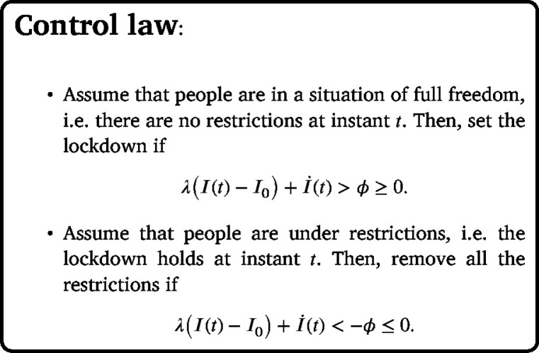
The time-varying rate is the result not only of biological but also of social factors. Hence, its value, as well as that of RN, contains also indication on the level of freedom and sociality of a population. In our mathematical description, it represents the unique parameter which can be modified by setting some restrictions. We will assume that it can take two values: in absence of restrictions (freedom) and during the lockdown. We also use to denote the desired equilibrium point, i.e. the target value for the number of infected . Ideally, one would like but this is not possible since, in absence of vaccines, it would require a lockdown of infinite temporal length. Our aim is instead to design a control law that maintains the system around a small value of , so that the number of people in intensive care can be managed by the health system, by mimicking the Australian strategy. Our approach is then formalized below. In its description, and are two design scalar parameters whose role to control the epidemic will be discussed in depth later on.
The control law proposed above relies on a sophisticated nonlinear control technique known as sliding-mode control, see also Appendix for details. Such an approach tries to bring (and maintain) the state trajectory on a given sliding surface, where the dynamics becomes completely independent of the model parameters and can be tuned accordingly to a desired target (this point is further described in second remark present at the end of Appendix A.1 in Appendix). In our case, the sliding surfaces for the SEIR and the SAIR models satisfy, respectively, the following equations
For what regards the control parameters, the scalar establishes how aggressive the control is. Large values of make the system approach faster to the sliding line. In addition, we also want to suitably alternate the periods of lockdown and freedom. This can be obtained by tuning the parameter . The choice is needed in practice since it induces chattering, i.e. an oscillation around . This is needed for avoiding an infinite frequency switching between freedom and lockdown: in any real-world situation, at least some days are required for changing the level of the restrictions. In practice, in our simulations it will be set to a conveniently low-value in order to obtain a suitable switching period. In its ideal version without such threshold, i.e. with , our control law activates a perfect sliding-mode whose functioning also requires some quite mild assumptions to be satisfied, as detailed in Appendix.
In what follows, theoretical results concerning the proposed algorithm will be first illustrated. Then, we will apply it to simulate the control of SARS-CoV-2 epidemic. Notably, we will see that the same law here described can be applied to either SEIR or SAIR guaranteeing the same control properties. Further generalizations will be studied in Appendix by introducing the SEAIR model, where the classes of exposed, asymptomatic and symptomatic infected are all included.
3. Results
3.1. Main theoretical findings
We summarize the two main theoretical results (described in detail in Appendix) regarding the proposed control law.
-
•
there always exist values of , known from a vague knowledge of SEIR or SAIR parameters, that ensure perfect convergence to the desired target when . Together with , the value of can then be adjusted to regulate the chattering phenomenon;
-
•
the epidemic control is robust since global convergence holds, i.e. the value is reached starting from any initial condition of either the SEIR or the SAIR model (at least if is small enough). In addition, the control is guaranteed also when system parameters are known with scarce precision.
3.2. Tuning the model and the control law
In what follows, due to space constraints, we focus on SEIR simulation and control. Results returned by the SAIR lead to the same conclusions illustrated below and can be found in Appendix.
SEIR parameters are defined by exploiting available information on COVID-19 dynamics, e.g. Gatto et al., 2020, Lavezzo et al., 2020 and Giordano, Blanchini, Bruno, Colaneri, Di Matteo, and Colaneri (2020). All the states are normalized, so that . The nominal value for is set to 0.05 which means that people heal on average in 20 days. To test the robustness of our control we will also make such rate vary in the interval (from two weeks to one month to heal). The nominal value for is 0.2 which means that people pass from exposed to infected in almost 5 days. The uncertainty interval for the incubation period is then (from three to 10 days) (Worldometer, 2021). To have insights on the value that the contact rate may assume during the freedom period, we use the reproduction numbers calculated by the Italian Ministry of Health during August, September and October, 2020 (Italian Ministry of Health, 2021). These months are especially significant since freedom of people much increased due to holiday relax and then also to the return to work and school. By monitoring the weekly reports present in Italian Ministry of Health (2021), the mean of the 95% upper bounds of the reproduction number RN turns out to be 1.3. This then defines through (2). We will also investigate the use of different reproduction numbers falling in the interval . Finally, to simulate a severe lockdown period, the contact rate during the restrictions is set to 0.01 with the uncertainty interval extending up to the value 0.02. This reflects the RN values measured on April 2020 during the lockdown in Italy, around 0.2–0.5 (Italian Ministry of Health, 2021). To simulate the epidemic, the initial value of the infected and exposed is 0.1% of the population.
For what regards the control law, the target is to maintain the value of to 0.2% of the population. For this purpose, we will set and we will adopt two values for , equal to 0.2 and 0.6, respectively.
To simulate the control of the SARS-CoV-2 spread, knowledge of and of its first-order derivative is assumed. Since the true number of infected is not perfectly known during an epidemic, in practice can be inferred from epidemiological measurements, like the number of hospitalized or diagnosed infected reported in Fig. 1. They are collected on a daily basis in Italy and Lombardy (the Italian region where most of the outbreak happened) during the first wave of infection, starting from March 1, 2020. Continuous-time profiles could be obtained by fitting such data e.g. through cubic smoothing splines (Wahba, 1990). Note that, when using the SAIR model, estimates of can be even more reliable since they do not need to include asymptomatic people who are in the most difficult class to be detected. The number of patients in critical care can be also much informative about COVID-19 dynamics and one strategy adopted in Pillonetto, Bisiacco, Palù, and Cobelli (2021) to estimate the number of infected is to assume it proportional to , i.e. . For future illustration purposes, it is useful to gain some information on this scale factor. In Italy, a robust lower bound for appears to be , a value that follows from simple considerations on the time-courses of diagnosed infected and people in ICUs (intensive care units) displayed in Fig. 1. Since the Italian population is around million, our control target then corresponds to maintaining the number of people in intensive care around 2400. This number is smaller than the critical threshold estimated in Italy as the 35% of the (almost) 10 000 places available in ICUs.
Fig. 1.
Number of diagnosed infected (left), hospitalized people (middle) and people in critical care (right) collected on a daily basis in Italy (solid line) and Lombardy (dashed) during the first wave of infection. The first instant corresponds to March 1, 2020. The first lockdown started on March 9, 2020, and the temporal interval of the figure then extends until its end.
3.3. Control of SARS-CoV-2
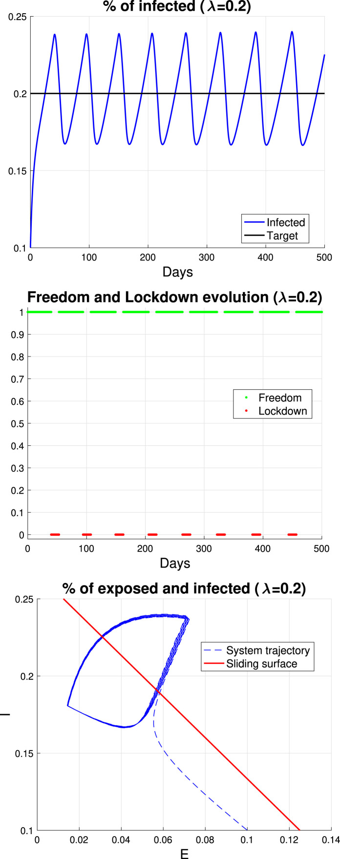
First, we simulate the model using the nominal values for the SEIR parameters and setting in the nonlinear control law. The top panel of Fig. 2 displays the percentage of infected (blue) and the target value (black). After a transient phase, one can see that starts oscillating around the desired level . The chattering is moderate, and also the infected peak (below 0.24%, an increment of the 20% of ) does not lead to exceed the critical threshold of people in intensive care. The middle panel then shows how the control law, in a totally automatic way, alternates freedom (green) and lockdown (red) periods. Interestingly, after getting rid of initial conditions effects, SARS-CoV-2 epidemic can be controlled using almost two months of freedom alternated with two weeks of severe restrictions. This is quite in line with the Australian scenario which appears so confirmed through our model. Results are not so sensitive to the adopted values of the contact rate during the freedom period. Setting , in place of 0.01, the freedom and lockdown periods increase by 3 and 5 days, respectively. Finally, the bottom panel shows how the trajectory of the exposed and infected evolves in the two-dimensional plane (blue) and how it approaches the sliding region (red), then moving around it.
Fig. 2.
Results returned by the nonlinear control law with . Top Percentage of infected (blue) and desired percentage (black) as a function of days. Middle Temporal evolution of freedom (green) and lockdown (red) periods. After a transient, almost two months of freedom and two weeks of severe lockdown are alternated. Bottom Trajectory describing how the percentage of exposed and infected varies in time (blue) and sliding surface (red). (For interpretation of the references to color in this figure legend, the reader is referred to the web version of this article.)
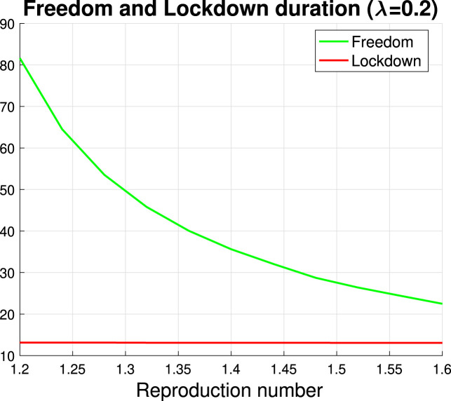
Fig. 3 shows the temporal lasting of the freedom (green) and lockdown (red) period as a function of the reproduction number (which was instead fixed to 1.3 to build Fig. 2). As expected, the freedom period required to control the epidemic with a precision error similar to that displayed in the top panel of Fig. 2 decays as the reproduction number increases. Indeed, larger values of (2) imply larger freedom or, also, a more aggressive pathogen agent. The freedom period seems to decay exponentially, while the lockdown duration slowly increases.
Fig. 3.
Temporal duration of the freedom (green) and lockdown (red) period, as a function of the reproduction number returned by the nonlinear control law with . The case with the reproduction number set to 1.3 corresponds to that detailed in Fig. 2. (For interpretation of the references to color in this figure legend, the reader is referred to the web version of this article.)
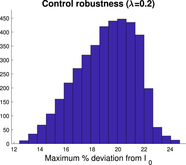
Fig. 4 illustrates the robustness of our control law. We simulated different SEIR models by making parameters and vary in the intervals already defined above. During any simulated epidemic the proposed control law was applied and the percentage deviation
was computed after the initial transient. The histogram of all these values is visible and one can see that the maximum percentage errors range from 12% to 24% (using the nominal parameter values it turns out 20%, as seen before). This well points out the effectiveness of our technique: without any knowledge on SEIR parameters, good control precision is always ensured.
Fig. 4.
Precisions in the control of the target value of infected using . The histogram contains the percentage deviations (computed after the initial transient) given by making SEIR parameters and vary on the intervals and , respectively. The figure thus shows that in any case the target can be well controlled: the error never exceeds 25%.
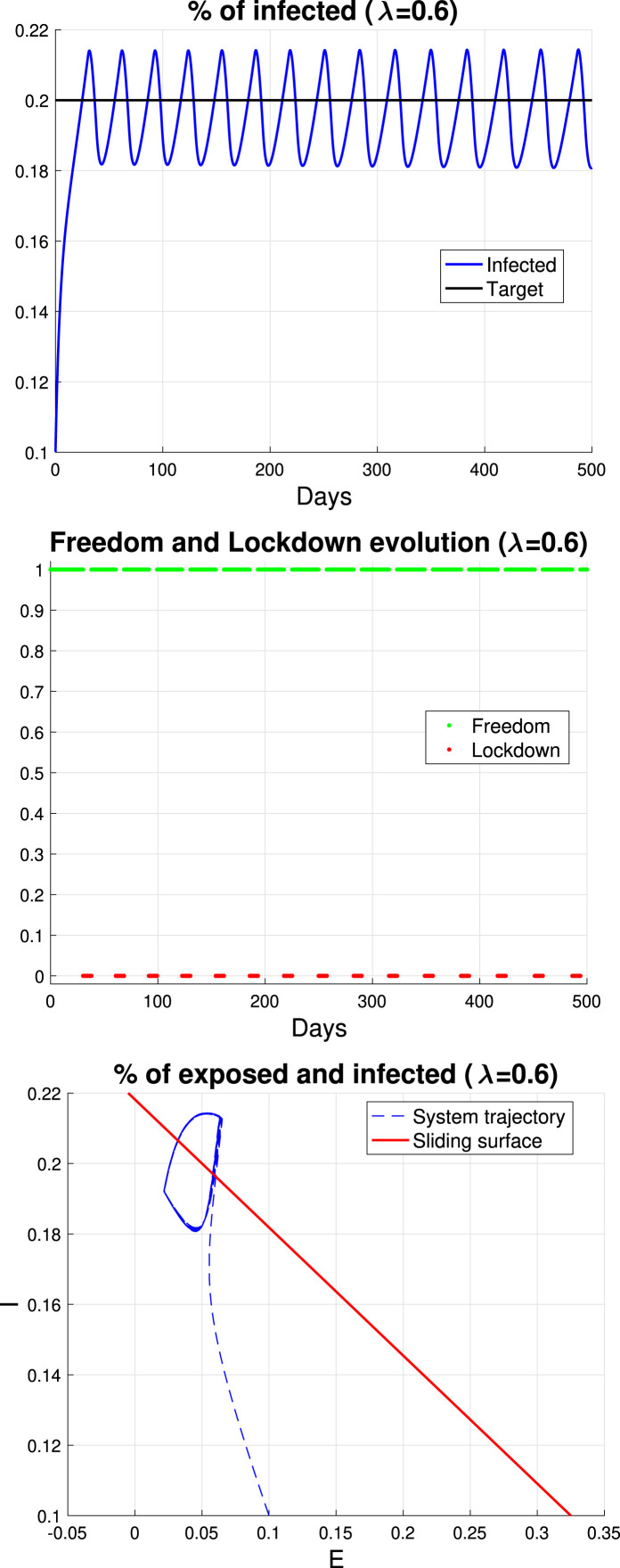
All of these figures were then redone by using a more aggressive control law, obtained by using . Comparing the top panels of Fig. 2, Fig. 5, one can see that the amplitude of the oscillation is now reduced. The middle panel of Fig. 5 shows that the control is now obtained with almost one month of freedom followed by one week of severe lockdown. This is even more in line with the Australian approach.
Fig. 5.
Results by the more aggressive control law with . Top Percentage of infected (blue) and desired percentage (black) as a function of days. In comparison with the top panel of Fig. 2 the amplitude of the oscillations of the infected is attenuated. Middle Temporal evolution of freedom (green) and lockdown (red) periods. After a transient, the control law now alternates almost one month of freedom and one week of severe lockdown. Bottom Trajectory describing how the percentage of exposed and infected varies in time (blue) and sliding surface (red). (For interpretation of the references to color in this figure legend, the reader is referred to the web version of this article.)
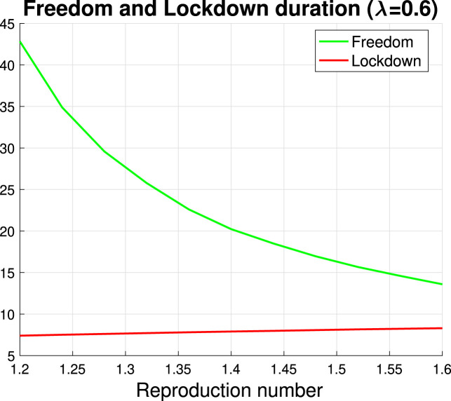
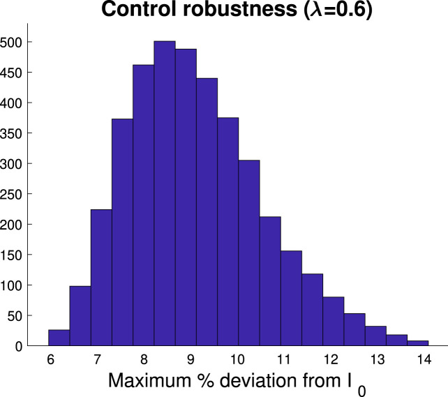
Fig. 6 plots the temporal duration of the freedom (green) and lockdown (red) period, as a function of the reproduction number. Comments similar to those regarding Fig. 3 hold. Finally, control robustness w.r.t. system parameters variations is documented in Fig. 7. Now, the maximum percentage error is smaller than 14%, hence ensuring high control precision.
Fig. 6.
Temporal duration of the freedom (green) and lockdown (red) period, as a function of the reproduction number returned by the nonlinear control law with . The case with the reproduction number set to 1.3 corresponds to that detailed in Fig. 5. (For interpretation of the references to color in this figure legend, the reader is referred to the web version of this article.)
Fig. 7.
Precisions in the control of the target value of infected using . The histogram contains the percentage deviations (computed after the initial transient) given by making SEIR parameters and vary on the intervals and , respectively. The figure thus shows that in any case the target can be well controlled: the error never exceeds 14%.
3.4. Effect of vaccines administration in improving the effectiveness of the control law
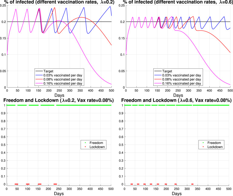
We also investigated the combined effect of the administration of vaccines and of the control law by simulating scenarios where a different number of people is vaccinated every day. For this purpose, one can just subtract and add the positive input to the equations governing and , respectively. We assume that the vaccine is administrated at and then becomes active in the population after two months, hence only for (Wang et al., 2021). The left and right top panels of Fig. 8 show the temporal evolution of the infected for and , respectively. Three different rates of vaccination are assumed, where or 0.16% of the population is vaccinated every day. In Italy the last scenario corresponds to vaccinate almost people per day. Using the smallest rate, one can see how the oscillations period tends to increase as time progresses, making staying longer below . In the other two cases, beyond this, the epidemic then quickly disappears. The left and right bottom panels of Fig. 8 illustrate the effect of the vaccines on the freedom and lockdown periods for (left) and (right) with the vaccination rate set to 0.08%.
Fig. 8.
Use of vaccines administrated at and with effect starting after two months. Top Percentages of infected and desired percentage (black) as a function of days for three different vaccination rates using (left) or (right). Bottom Temporal evolution of freedom (green) and lockdown (red) periods for (left) and (right) with the vaccination rate set to 0.08%. (For interpretation of the references to color in this figure legend, the reader is referred to the web version of this article.)
3.5. Final remarks on obtained results with and without vaccines
We have seen in the top panels of Fig. 8 that trajectories of the infected generated by our control law in presence of vaccines administration are aperiodic. Actually, this feature also holds in absence of vaccines: in the previous figures, e.g. top panel of Fig. 2, they seem periodic only because of the limited time range there adopted. This is due to the following reasons:
-
•
oscillations are the consequence of the use of non-ideal sliding mode connected with the chattering phenomenon induced by the choice . Specifically, it induces an oscillation around the nominal trajectory on the sliding line which is moving linearly, and exponentially fast in time, along the plane towards the equilibrium point. Apart from the initial brief transient phase, the infected peak would be equal to in case of , while in practice it turns out to be a little larger because of the chattering;
-
•
since is monotone decreasing, the duty-cycle, defined as the ratio between the lockdown time and the total time of the oscillations, is continuously decreasing (this is visible only after a certain number of oscillations). This happens because, as time increases, the effective reproduction number, that corresponds to the product between the basic reproduction number and (Fine, 1993), is slowly decreasing both during the freedom and lockdown period. Our simulations also show that the freedom phase is more sensitive to variations of , hence the period of the oscillations increases while the duty-cycle decreases as time progresses;
-
•
the lockdown threshold is not reached forever. In fact, when becomes small enough, the epidemic dies down on its own, without the need of further lockdowns. Hence, the equilibrium point cannot be any longer maintained, the trajectory of infected leaves the sliding line and tends to zero (epidemic extinction).
Regarding the last point mentioned above, the fact that the control is not maintained forever has also consequences on the study of epidemic final size (Bliman and Duprez, 2021, Lauro et al., 2021, Morris et al., 2021). In particular, the control law will be disabled after the so-called herd immunity will take place, i.e. when the effective reproduction number during the freedom period is equal to one (Fine, 1993). Specifically, this will happen at the time-instant such that . The fact that attainment of the herd immunity is eventually guaranteed by the proposed control law also implies that the arising of another epidemic wave is prevented. The exact final value will then depend on the social behavior after , but it will likely be a little smaller than since the epidemic will be going towards extinction.
Note also that in its ideal version (i.e. with no chattering), and neglecting the transient phase, the control law here described minimizes the epidemic duration subject to the constraint . In fact, if for any , one has , so the epidemic length is given by . It is easily seen that any other choice of , subject to the constraint , leads to a longer epidemic duration.
4. Conclusions
Differently from the strategies adopted in USA and Europe, the Australian model tends to suddenly set short-term severe lockdowns as soon as the number of infected exceeds a certain threshold. We have shown that this strategy can be described in mathematical terms providing a connection with sliding-mode, an important branch of nonlinear control. From this work, one cannot argue that the Australian approach is the best one. However, this paper develops some mathematical and simulation tools that strengthen it, showing that it can likely be a valid alternative solution for other countries. Our analysis also generalizes and improves it since any value of infected to be controlled can be chosen. Our study permits also to simulate interesting scenarios of action which can also include the effect of vaccines administration. It leads to a robust control law, having high-performance also in presence of scarce knowledge on the parameters which regulate SARS-CoV-2 dynamics. When a certain threshold related to the number of either infected or people in intensive care is overcome, the epidemic can be promptly controlled. In fact, from any initial condition the control law permits to come back to the desired equilibrium point with an exponential speed. Such a control strategy reveals advantages in terms of sociability: also in other countries people could prefer to undergo a severe but short-term lockdown (e.g. lasting just one or two weeks) to then enjoy a much larger period of freedom (e.g. of one or two months).
Declaration of Competing Interest
The authors declare that they have no known competing financial interests or personal relationships that could have appeared to influence the work reported in this paper.
Appendix.
A.1. SEIR control
We report the theoretical analysis concerning the SEIR while the SAIR and SEAIR cases are discussed in the last part of Appendix.
In (1) we are interested in establishing the (possible) existence of non-zero equilibrium points for the only variables . Let the equilibrium values be and , respectively. From , it holds that , while leads to . These equations admit at least one positive solution if and only if
| (5) |
Letting , one has . Recall that only two values are allowed for : (lockdown) and (freedom), so in case of a full freedom, the epidemic spread requires , while the lockdown is successful only if , so we need to assume
| (6) |
Therefore the positive equilibrium point exists for , and we are only interested in situations in which . Let us briefly discuss the case where such inequality is not satisfied. If the lockdown is not successful and we simply cannot face the epidemic spread, but only slow it. If , there is no need to set a lockdown, as the epidemic will disappear on its own. Under the assumption (6) we can thus define through
| (7) |
with having opposite signs in the freedom/lockdown cases. By rewriting (1) in terms of and , one has
| (8) |
| (9) |
that implies
| (10) |
| (11) |
with . Then, exploiting the following change of variables
one obtains the simple linear system
| (12) |
Some results from Sliding Modes Control Theory are now briefly recalled and then also specialized to the two-dimensional case.
Proposition 1 Equivalent Input on a Sliding Surface —
Let (which is equivalent to ) be the desired sliding surface. The equivalent input which allows to remain in the sliding surface is obtained by imposing and is therefore given by
(13) and this leads to
By defining
| (14) |
the eigenvalues of are given by . The negative eigenvalue ensures asymptotic stability, and this requires
In other words, implies for any if , and this implies for any , so that after some easy computations
| (15) |
which makes the dynamics on the sliding line expressed by a linear system with eigenvalue . So, once has been chosen, it suffices to evaluate through (14) in order to obtain the expression of the sliding line and to ensure that the dynamics of on the sliding line only depends on , and is therefore completely independent of the system parameters .
For what regards the control law, following Sliding Modes Theory, a simple possibility is the discontinuous law
| (16) |
where is any uniformly lower-bounded (by some positive constant ) function, and where the (possible) dependence of on both and (because its value could be different over and under the sliding line) have been put in evidence. For simplicity sake, in the following we will omit the arguments of , when not strictly necessary. Now, we need to investigate when this law is able to reach (and then to maintain) the state trajectory on the sliding surface.
Proposition 2 Sufficient Condition for the (LOCAL) Sliding Establishment —
Let be a subset (possibly either only a point or the whole line) of the (stabilizing) sliding line containing the equilibrium point . Assume that a closed neighborhood of exists such that
- •
is an invariant region (which means implies )
- •
for any it holds , for some
Then the control law (16) permits to reach in finite time, starting from any initial condition and then the trajectory never escapes from .
Proof
From (12) it easily follows
which is surely verified if
and easily implies for some . From onwards, cannot become different from zero, otherwise a contradiction would arise as a consequence of the opposite signs of and of its derivative over and under . The invariance property is required both for the inequality validity until the sliding line is reached, and, together with the monotone (exponential) movement on towards (see (15)), for avoiding to exit from along the sliding line, once is reached. ■
The following corollary is then immediately obtained.
Corollary 1 Sufficient Condition for the (GLOBAL) Sliding Establishment —
Let satisfy the assumptions of Proposition 2 , and assume that for any , excluding the origin, the corresponding trajectory reaches in finite time. Then the sliding establishment is globally guaranteed.
The following proposition is our main result. It shows when the control law (16) satisfies the conditions reported above for either local or global sliding. The proof is quite technical and shows how (16) and the sliding line introduced above coincide, respectively, with the control law exposed before (4) and with (4) itself.
Proposition 3 Effectiveness of the Control Law (16) —
For small enough, the control law (16) satisfies the conditions for the global sliding establishment. Furthermore, the same control law satisfies the conditions for the local sliding establishment for any choice of and of the SEIR parameters.
Proof
First, recall the definition of the scalar , i.e.
Now, we want to prove that the control law (16) satisfies the conditions expressed in Proposition 2 for any and the conditions expressed in Corollary 1 if is small enough. The proof is split into some steps.
Step 1 [Computation of , , and ]. First of all, can be expressed in terms of . In fact
from which
Recalling also and (7), it holds that , which leads, in case of freedom and lockdown respectively, to
Therefore the control law
(17) easily follows, together with the sliding line expression
(18) and with the expression of the sign of
The last expression shows why no measurements on are needed: all the information about is included in the knowledge of the pair . Above, is exactly the eigenvalue we want to obtain, whose choice is completely independent of the knowledge of . Finally, recalling the expression of , it holds that
Step 2 [The conditions in Proposition 2 (in case of )]. The conditions to be checked become
which, recalling the expression of reported in the previous step, allows to express the previous implications as follows
Now assume . After some computations we obtain, equivalently
Step 3 [Computation of the region satisfying the conditions in Proposition 2 (in case of )]. In view of the previous results, we need to consider three straight lines of the form , with
Consider also other two lines defined by
where the first one expresses all the (possible) equilibrium points, while the second one is needed since could be negative. It is easy to see that, for and small enough, a point (continuously depending on , and tending to the origin as and go to zero) exists such that
while it holds
Hence, the first implication ( implies ) is verified in the closed region
which has a piecewise-linear boundary. Since implies both that is increasing and is decreasing, this prevents any trajectory to cross either the line or the line , for any such that .
Analogously, for and small enough, also a point (with the same properties has) exists such that
and the second implication ( implies ) is verified in the closed region
which has a piecewise-linear boundary. Since implies both that is decreasing and is increasing, this prevents any trajectory to cross either the line or the line , for any such that . So it holds a fortiori in the whole region itself.
Now it suffices to choose and to obtain the region as a closed neighborhood of almost all the sliding line satisfying the conditions of Proposition 2. Recall that continuously depend on and that for . Then, choosing small enough, we can obtain arbitrarily small. In other words, at least an interval exists such that the assumptions of Proposition 2 are satisfied in the aforementioned region, which contains almost all the sliding line except for an arbitrarily small segment.
Step 4 [Global convergence to the sliding line if is small enough].
The proof that, for any , the couple will eventually reach the aforementioned region in finite time (hence ensuring the sliding functioning after a finite time for any initial condition, at least for small enough) is simple but tedious. It is therefore omitted.
Below, we now verify that, independently of the system parameters and of , both the conditions in Proposition 2 are always satisfied. Such a local property is needed for allowing the arising of sliding modes, even though it cannot guarantee it in a global sense, i.e. starting from any initial condition.
Step 5 [Local (at least) convergence to the sliding line for any ].
Starting from , we can express , and resorting to a change of variables , with , the differential equations can be rewritten as follows
Recalling (see Step 1), where depends on both (through ) and the lockdown/freedom state, let us assume and denote with the minimum value can assume. Choose now any such that
and consider the closed neighborhood of given by
From
it follows , so that implies that monotonically converges to zero in finite time, if forever. But this easily follows from , by analyzing the evolution of which moves towards the straight-line . This does not allow to escape from , hence showing that both the conditions in Proposition 2 are always satisfied. ■
Some remarks are now in order.
-
•
It has been shown that the sliding line attracts all the trajectories in finite time for belonging to a suitable (small) interval. However, this does not prevent the possibility of obtaining a sliding functioning also for other (possibly all) values of . In fact, Proposition 3 states only a sufficient condition. Note however that we have not only characterized some situations in which the sliding-mode technique can be applied, but also, through Proposition 3, that any choice of and of the SEIR parameters is compatible with the existence of a sliding-mode evolution.
-
•
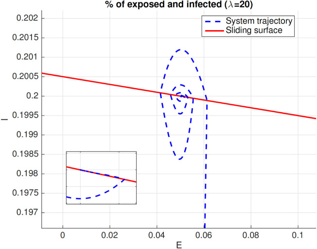
Once the sliding line is reached at some point , two scenarios are possible. Either the trajectory crosses the sliding line (in case the point does not belong to the attractive neighborhood of the equilibrium point - see Proposition 2), or it remains on the sliding line forever (actually until reaches the value and the epidemic is quickly going towards its extinction). In the latter case, evolves accordingly to the exponential monotone behavior described by , where satisfies (see (15)). Such a behavior becomes therefore completely independent of the (possibly unknown) values of the SEIR parameters, from onwards. What depends instead on is the sliding line expression and, in particular, the value of . This latter is however of no interest since the target is to control the steady-state value . The parameters values could instead influence both the transient phase and the establishment of the sliding-mode, but our simulations show that it is obtained in all the cases of interest. It is worth also remarking that reaching the sliding line does not guarantee the sliding-mode establishment. In fact, usually only an attractive neighborhood is available and some line crossings can occur before the sliding mode takes place also using perfect sliding, i.e. avoiding chattering by setting . This phenomenon is also graphically illustrated in Fig. 9.
-
•
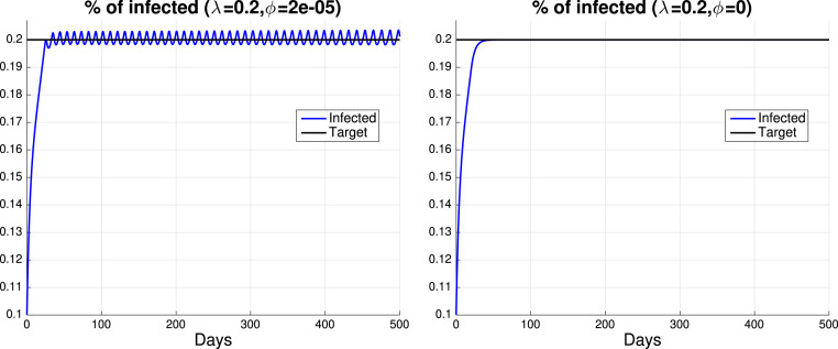
From a practical viewpoint, one needs to alternate lockdown and freedom periods, and this leads to an oscillation around . This can be obtained by modifying the control law as follows: if then , if then , otherwise remains locked at the previous value. Here, represents a threshold that can be suitably tuned by using the parameter entering the control law. This means that we can modulate the amplitude (and the duration) of the oscillations to define lockdown/freedom periods of practical meaning, without significantly affecting either the mean value (that remains almost equal to ) or the duty-cycle of the ON/OFF signal associated with the lockdown presence or absence. This is the well-known chattering phenomenon, which consists of finite-frequency oscillations around the sliding surface (the theoretical frequency in the ideal case would be infinite). An illustration is given in Fig. 10 where the effect of two different values of on the control of the infected is illustrated.
-
•
Once the steady-state values are reached, the system behaves like if assumes exactly the (time-varying) value given by (5). In other words, the structure of the control law guarantees in an automatic way that the reproduction number becomes exactly equal to .
-
•The condition cannot hold forever since is strictly decreasing. At the epidemic beginning , so satisfies if . But holds true until becomes small enough to be no longer able to feed in such a way that the equilibrium point is maintained. In fact, is monotone and strictly decreasing, so if for some (actually and , as already previously discussed), the evolution in case of full freedom satisfies
which leads to the epidemic extinction without further control (lockdowns) actions. This means that at a certain time instant the evolution will escape from the sliding line. This is not a problem: it corresponds to epidemic extinction and control laws are no longer required. As becomes smaller, the freedom period becomes longer and the duty-cycle tends to privilege freedom to lockdown as time advances. Then, at a certain temporal instant the lockdown disappears and the trajectory of infected people leaves the steady-state value when the epidemic is going towards extinction. Examples are the red and magenta lines in the top panels of Fig. 8 and the bottom panels in the same figure where these phenomena are accelerated by vaccines administration that makes decrease faster.(19)
Fig. 9.
State trajectories on the -plane with same setting used to build Fig. 2 except that is set to zero (no chattering phenomenon can happen) and . The smaller part of the figure provides a zoom showing how the trajectory eventually enters the sliding line and then remains over it, after some previous sliding line crossings.
Fig. 10.
Percentage of infected (blue) and desired percentage (black) as a function of days. The same setting used to build the top panel of Fig. 2 is adopted except that the parameter entering the control law is set to smaller values. (For interpretation of the references to color in this figure legend, the reader is referred to the web version of this article.)
A.2. SAIR and SEAIR control
A.2.1. SAIR model
Now, consider the SAIR model given by
| (20a) |
| (20b) |
| (20c) |
| (20d) |
Similarly to what done in the SEIR case, first we focus only on the equations related to the evolutions of to determine the structure of the possible non-zero equilibrium points. The conditions for their existence are
which implies
Hence, we can define
which requires
in order to obtain having opposite signs in case of freedom and lockdown (at least until is large enough). Simple calculations provide
which, by introducing nominal values and a matrix defining our sliding surface, allows to obtain
which implies
The equivalent input is given by
and leads to the following autonomous linear system
whose eigenvalues are . In particular, is given by
and makes
We thus obtain
which implies the same control law obtained in the SEIR case, with the constant playing exactly the same role previously discussed, i.e.
The only thing that changes is the relationship between the eigenvalue , the model parameters and the constant . Proposition 3 is satisfied in this case too, with arguments omitted due to space constraints and because they are quite similar to those developed in the SEIR case.
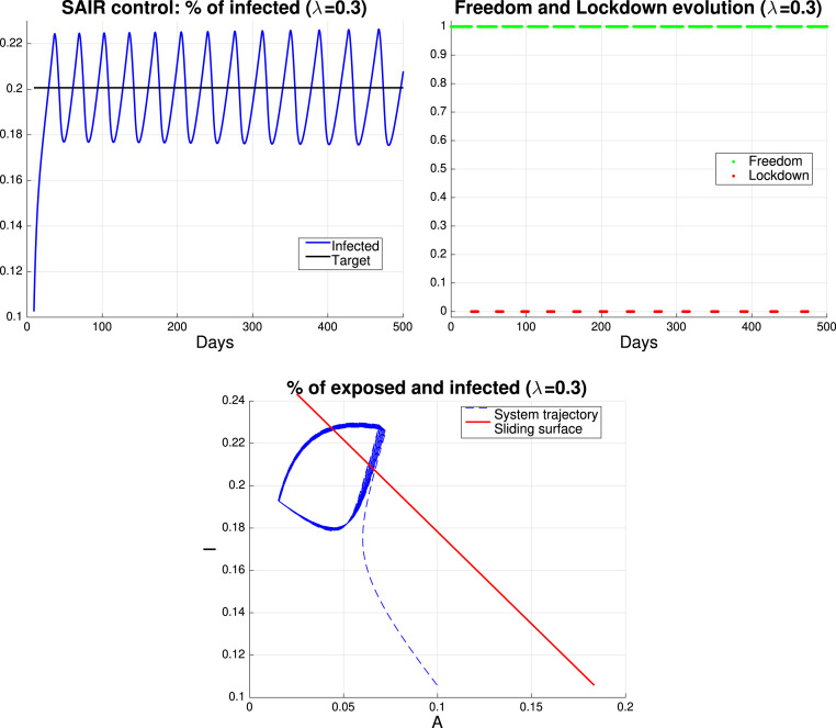
Now, we report a simulation concerning SAIR control with system parameters all set to values well supported in the literature (Gatto et al., 2020, Giordano et al., 2020, Lavezzo et al., 2020, Worldometer, 2021). We set (on average asymptomatic become symptomatic in 5 days), (asymptomatic heal in two weeks) and (symptomatic heal in 20 days). The same reproduction numbers adopted in the SEIR case then define the contact rate during the freedom and lockdown periods. As documented in Fig. 11, the choice allows to control SARS-CoV-2 epidemic alternating almost 32 days of freedom and 8 days of lockdown.
Fig. 11.
Control of SAIR model. Results returned by the nonlinear control law with . Top left Percentage of infected (blue) and desired percentage (black) as a function of days. Top right Temporal evolution of freedom (green) and lockdown (red) periods. After a transient, almost one month of freedom and one week of severe lockdown are alternated. Bottom Trajectory describing how the percentage of exposed, who became asymptomatic, and of infected varies in time (blue) and sliding surface (red). (For interpretation of the references to color in this figure legend, the reader is referred to the web version of this article.)
A.2.2. SEAIR model
The SEAIR model is a generalization of the SEIR and SAIR that contains both the exposed and the asymptomatic class. It is given by
| (21a) |
| (21b) |
| (21c) |
| (21d) |
| (21e) |
In this case, we have to focus on three differential equations governing in order to investigate non-zero equilibrium points:
Now, we define through
which requires
to obtain having opposite signs. Simple calculations lead to
In this case, two coefficients are needed in the matrix , i.e.
and this implies
The equivalent input and the matrix are given by
hence
with
The characteristic polynomial of is
which uniquely defines in terms of (one-to-one linear correspondence). Stability requires .
Let us now express in terms of the only measurable variable . To this aim, first we write by resorting to the equation of :
Then, exploiting also the equation of , one has
which implies
from which
This implies
Recalling the expressions of , this leads to the simple expression
which represents the natural generalization of the SAIR and SEIR cases and defines the following (more sophisticated) control law
with . The sliding surface
can be also formulated in terms of the state variables as follows
One can notice the analogy with the previous control law and sliding surface expression, but the difference is that now the second order derivative of is also needed. This can make control harder since it could be difficult to obtain good estimates of . However, using to indicate a generic positive scalar, one can see that
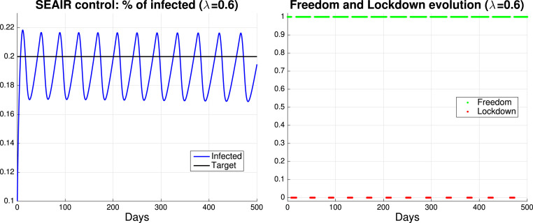
with that now can be arbitrary positive real numbers. As , we obtain that disappears and the control law reduces to that seen before. Under a theoretical perspective, is not admissible since no real sliding mode (the movement on the sliding surface after a transient phase) is possible. However, we are not interested in a pure sliding mode as we want to alternate periods of lockdown/freedom of significant duration. In this respect, while the presence of is important since it contains the information about the trend, choosing may be an admissible choice. In fact, from a practical viewpoint, if the aim is just to alternate periods of lockdown/freedom of significant duration, by resorting to a very small or to may lead to small differences in the control. Simulation results suggest that this happens. In particular, we simulated SEAIR control setting (exposed become asymptomatic in 3 days on average), (asymptomatic become symptomatic in 3 days), (asymptomatic heal in two weeks) and (symptomatic heal in 20 days). The same reproduction numbers adopted in the SEIR and SAIR case then define the contact rate during the freedom and lockdown periods. Fig. 12 shows the results obtained with . SARS-CoV-2 is now controlled by alternating almost 35 days of freedom and 9 days of lockdown.
Fig. 12.
Control of SEAIR model. Results returned by the nonlinear control law with and . Left Percentage of infected (blue) and desired percentage (black) as a function of days. Right Temporal evolution of freedom (green) and lockdown (red) periods. After a transient, almost one month of freedom and one week of severe lockdown are alternated. (For interpretation of the references to color in this figure legend, the reader is referred to the web version of this article.)
Data availability
All data used in this manuscript are publicly available at https://github.com/pcm-dpc/COVID-19
References
- A. Ibeas, A., de la Sen, M., & Alonso-Quesada, S. (2013). Sliding mode robust control of SEIR epidemic models. In 21st Iranian Conference on Electrical Engineering (ICEE) (pp. 1–6).
- Anastassopoulou C., Russo L., Tsakris A., Siettos C. Data-based analysis, modelling and forecasting of the COVID-19 outbreak. PLoS. 2020;15 doi: 10.1371/journal.pone.0230405. [DOI] [PMC free article] [PubMed] [Google Scholar]
- Berger T. 2020. Feedback control of the COVID-19 pandemic with guaranteed non-exceeding ICU capacity. arXiv. arXiv:2008.09426. [DOI] [PMC free article] [PubMed] [Google Scholar]
- Bertuzzo E., Casagrandi R., M. G., Rodriguez-Iturbe I., Rinaldo A. On spatially explicit models of cholera epidemics. Journal of the Royal Society Interface. 2010;7:321–333. doi: 10.1098/rsif.2009.0204. URL http://dx.medra.org/10.1098/rsif.2009.0204. [DOI] [PMC free article] [PubMed] [Google Scholar]
- Bliman P., Duprez M. How best can finite-time social distancing reduce epidemic final size? Journal of Theoretical Biology. 2021;511 doi: 10.1016/j.jtbi.2020.110557. [DOI] [PMC free article] [PubMed] [Google Scholar]
- Bootsma M., Ferguson N. The effect of public health measures on the 1918 influenza pandemic in US cities. Proceedings of the National Academy of Sciences. 2007;104(18):7588–7593. doi: 10.1073/pnas.0611071104. [DOI] [PMC free article] [PubMed] [Google Scholar]
- Borri A., Palumbo P., Papa F., Possieri C. Optimal design of lock-down and reopening policies for early-stage epidemics through SIR-D models. Annual Reviews in Control. 2021 doi: 10.1016/j.arcontrol.2020.12.002. [DOI] [PMC free article] [PubMed] [Google Scholar]
- Capasso V., Serio G. A generalization of the kermack-mckendrick deterministic epidemic model. Mathematical Biosciences. 2007;42(1–2):43–61. [Google Scholar]
- Casella F. 2020. Can the COVID-19 epidemic be controlled on the basis of daily test reports? ArXiv. arXiv:2003.06967. [Google Scholar]
- Cave D. One case, total lockdown: Australia?s lessons for a pandemic world. The New York Times. 2021 https://www.nytimes.com/2021/02/01/world/australia/perth-lockdown.html. [Google Scholar]
- Diekmann O., Heesterbeek J., Metz J. On the definition and the computation of the basic reproduction ratio in models for infectious diseases in heterogeneous populations. Journal of Mathematical Biology. 1990;28:365–382. doi: 10.1007/BF00178324. [DOI] [PubMed] [Google Scholar]
- Fine P. Herd immunity: History, theory, practice. Epidemiologic Reviews. 1993;15:265–302. doi: 10.1093/oxfordjournals.epirev.a036121. [DOI] [PubMed] [Google Scholar]
- Garetto M., Leonardi E., Torrisi G. A time-modulated hawkes process to model the spread of COVID-19 and the impact of countermeasures. Annual Reviews in Control. 2021 doi: 10.1016/j.arcontrol.2021.02.002. [DOI] [PMC free article] [PubMed] [Google Scholar]
- Gatto M., Bertuzzo E., Mari L., Miccoli S., Carraro L., Casagrandi R., et al. Spread and dynamics of the COVID-19 epidemic in Italy: Effects of emergency containment measures. Proceedings of the National Academy of Sciences. 2020;117(19):10484–10491. doi: 10.1073/pnas.2004978117. [DOI] [PMC free article] [PubMed] [Google Scholar]
- Giordano G., Blanchini F., Bruno R., Colaneri P., Di Matteo A., Colaneri M. Modelling the COVID-19 epidemic and implementation of population-wide interventions in Italy. Nature Medicine. 2020:1–6. doi: 10.1038/s41591-020-0883-7. [DOI] [PMC free article] [PubMed] [Google Scholar]
- Gondim J., Machado L. Optimal quarantine strategies for the COVID-19 pandemic in a population with a discrete age structure. Chaos, Solitons & Fractals. 2020;140 doi: 10.1016/j.chaos.2020.110166. [DOI] [PMC free article] [PubMed] [Google Scholar]
- Guan W., Ni Z., Hu Y., Liang W., Ou C., He J., et al. Clinical characteristics of coronavirus disease 2019 in China. New England Journal of Medicine. 2020;382(18):1708–1720. doi: 10.1056/NEJMoa2002032. [DOI] [PMC free article] [PubMed] [Google Scholar]
- Italian Ministry of Health . 2021. Website monitoring COVID-19 epidemic evolution in Italy. http://www.salute.gov.it/ [Google Scholar]
- Keeling M., Eames K. Networks and epidemic models. Journal of the Royal Society Interface. 2005;2(4):295–307. doi: 10.1098/rsif.2005.0051. [DOI] [PMC free article] [PubMed] [Google Scholar]
- Kernack W., McKendrick A. A contribution to the mathematical theory of epidemics. Proceedings of the Royal Society of London, Series A. 1927;115(772):700–721. [Google Scholar]
- Kohler J., Schwenkel L., Koch A., Berberich J., Pauli P., Allgower F. Robust and optimal predictive control of the COVID-19 outbreak. Annual Reviews in Control. 2021 doi: 10.1016/j.arcontrol.2020.11.002. [DOI] [PMC free article] [PubMed] [Google Scholar]
- Korobeinikov A., Maini P. Non-linear incidence and stability of infectious disease models. Mathematical Medicine and Biology: A Journal of the IMA. 2005;22(2):113–128. doi: 10.1093/imammb/dqi001. [DOI] [PubMed] [Google Scholar]
- L. Pilat D.C., Juanola M. Perth, peel, SW in lockdown after hotel quarantine worker tests positive to COVID-19. WAtoday. 2021 https://www.watoday.com.au/national/western-australia/much-of-wa-going-into-lockdown-from-6pm-after-hotel-quarantine-worker-tests-positive-20210131-p56y78.html. [Google Scholar]
- Lauro F.D., Kiss I., Miller J. Optimal timing of one-shot interventions for epidemic control. PLoS Computational Biology. 2021;17 doi: 10.1371/journal.pcbi.1008763. [DOI] [PMC free article] [PubMed] [Google Scholar]
- Lavezzo E., Franchin E., al. E.C. Suppression of a SARS-CoV-2 outbreak in the Italian municipality of Vo’. Nature. 2020 doi: 10.1038/s41586-020-2488-1. [DOI] [PubMed] [Google Scholar]
- Lin Q., Zhao S., Gao D., Lou Y., Yang S., Musa S.S., et al. A conceptual model for the coronavirus disease 2019 (COVID-19) outbreak in wuhan, China with individual reaction and governmental action. International Journal of Infectious Diseases. 2020;93:211–216. doi: 10.1016/j.ijid.2020.02.058. [DOI] [PMC free article] [PubMed] [Google Scholar]
- Liu W., Hethcote H., Levin S. Non-linear incidence and stability of infectious disease models. Dynamical Behavior of Epidemiological Models with Nonlinear Incidence Rates. 1987;25(4):359–380. doi: 10.1007/BF00277162. [DOI] [PubMed] [Google Scholar]
- Mari L., Casagrandi R., Bertuzzo E., Rinaldo A., Gatto M. Floquet theory for seasonal environmental forcing of spatially explicit waterborne epidemics. Theoretical Ecology. 2014;7(4):351–365. [Google Scholar]
- Mari L., Casagrandi R., Bertuzzo E., Rinaldo A., Gatto M. Conditions for transient epidemics of waterborne disease in spatially explicit systems. Royal Society Open Science. 2019;6(5) doi: 10.1098/rsos.181517. [DOI] [PMC free article] [PubMed] [Google Scholar]
- Morris D., Rossine F., Plotkin J., Levin S. Optimal, near-optimal, and robust epidemic control. Communications Physics. 2021;4 [Google Scholar]
- Nunez S., Inthamoussou F., Valenciaga F., De Battista H., Garelli F. Potentials of constrained sliding mode control as an intervention guide to manage COVID19 spread. Biomedical Signal Processing and Control. 2021;67 doi: 10.1016/j.bspc.2021.102557. [DOI] [PMC free article] [PubMed] [Google Scholar]
- O’Sullivan D., Gahegan M., Exeter D., Adams B. Spatially explicit models for exploring COVID-19 lockdown strategies. Transactions in GIS. 2020:1–34. doi: 10.1111/tgis.12660. [DOI] [PMC free article] [PubMed] [Google Scholar]
- Pastor-Satorras R., Castellano C., Van Mieghem P., Vespignani A. Epidemic processes in complex networks. Reviews of Modern Physics. 2015;87(925) [Google Scholar]
- Pastore Piontti A., Gomes M., Samay N., Perra N., Vespignani A. The infection tree of global epidemics. Networking Science. 2014;2(1):132–137. [Google Scholar]
- Pellis L., Ball F., Bansal S., Eames K., House T., Isham V., et al. Eight challenges for network epidemic model. Epidemics. 2015;10:58–62. doi: 10.1016/j.epidem.2014.07.003. [DOI] [PubMed] [Google Scholar]
- Pillonetto G., Bisiacco M., Palù G., Cobelli C. Tracking the time course of reproduction number and lockdown’s effect during SARS-CoV-2 epidemic: nonparametric estimation. Scientific Reports. 2021;11(1):9772. doi: 10.1038/s41598-021-89014-9. [DOI] [PMC free article] [PubMed] [Google Scholar]
- Riley S., Eames K., Isham V., Mollison D., Trapman P. Five challenges for spatial epidemic models. Epidemics. 2015;10(3):68–71. doi: 10.1016/j.epidem.2014.07.001. [DOI] [PMC free article] [PubMed] [Google Scholar]
- Sadeghi M., Greene J., Sontag E. Universal features of epidemic models under social distancing guidelines. Annual Reviews in Control. 2021 doi: 10.1016/j.arcontrol.2021.04.004. [DOI] [PMC free article] [PubMed] [Google Scholar]
- Sharifi M., Moradi H. Nonlinear robust adaptive sliding mode control of influenza epidemic in the presence of uncertainty. Journal of Process Control. 2017;56:48–57. [Google Scholar]
- Shtessel Y. Springer; N.J., USA: 2014. Sliding mode control and observation. [Google Scholar]
- Tsay C., Lejarza F., Stadtherr M., Baldea M. Modeling, state estimation, and optimal control for the US COVID-19 outbreak. Scientific Reports. 2020;10 doi: 10.1038/s41598-020-67459-8. [DOI] [PMC free article] [PubMed] [Google Scholar]
- Van den Driesschea P., Watmoughb J. Reproduction numbers and sub-threshold endemic equilibria for compartmental models of disease transmission. Mathematical Biosciences. 2002;180:29–48. doi: 10.1016/s0025-5564(02)00108-6. [DOI] [PubMed] [Google Scholar]
- Velavan T., Meyer C. The COVID-19 epidemic. Tropical Medicine & International Health. 2020;25:278–280. doi: 10.1111/tmi.13383. [DOI] [PMC free article] [PubMed] [Google Scholar]
- Wahba G. SIAM; Philadelphia: 1990. Spline models for observational data. [Google Scholar]
- Wallinga J., Teunis P. Different epidemic curves for severe acute respiratory syndrome reveal similar impacts of control measures. American Journal of Epidemiology. 2004;160(6):509–516. doi: 10.1093/aje/kwh255. [DOI] [PMC free article] [PubMed] [Google Scholar]
- Wang Y., Chen Y., Quin Q. Unique epidemiological and clinical features of the emerging 2019 novel coronavirus pneumonia (COVID-19) implicate special control measures. Journal of Medical Virology. 2020;92:568–576. doi: 10.1002/jmv.25748. [DOI] [PMC free article] [PubMed] [Google Scholar]
- Wang Z., Schmidt F., Weisblum Y., et al. mRNA vaccine-elicited antibodies to SARS-CoV-2 and circulating variants. Nature. 2021 doi: 10.1038/s41586-021-03324-6. [DOI] [PMC free article] [PubMed] [Google Scholar]
- Weitz J.S., Beckett S.J., Coenen A.R., Demory D., Dominguez-Mirazo M., Dushoff J., et al. Modeling shield immunity to reduce COVID-19 epidemic spread. Nature Medicine. 2020 doi: 10.1038/s41591-020-0895-3. [DOI] [PMC free article] [PubMed] [Google Scholar]
- Wittkowski K. The first three months of the COVID-19 epidemic: Epidemiological evidence for two separate strains of SARS-CoV-2 viruses spreading and implications for prevention strategies. MedRxiv. 2020 doi: 10.1101/2020.03.28.20036715. [DOI] [PMC free article] [PubMed] [Google Scholar]
- Worldometer . 2021. Website on coronavirus incubation period. https://www.worldometers.info/coronavirus/coronavirus-incubation-period/ [Google Scholar]
- Wu Z., McGoogan J. Characteristics of and important lessons from the coronavirus disease 2019 (COVID-19) outbreak in China: summary of a report of 72314 cases from the Chinese center for disease control and prevention. JAMA. 2020;323:1239–1242. doi: 10.1001/jama.2020.2648. [DOI] [PubMed] [Google Scholar]
- Xiao Y., Xu X., Tang S. Sliding mode control of outbreaks of emerging infectious diseases. Bulletin of Mathematical Biology. 2012;74:2403–2422. doi: 10.1007/s11538-012-9758-5. [DOI] [PubMed] [Google Scholar]
- Zhou F., Yu T., Du R., Fan G., Liu Z., Xiang J., et al. Clinical course and risk factors for mortality of adult inpatients with COVID-19 in Wuhan, China: a retrospective cohort study. The Lancet. 2020;395:1054–1062. doi: 10.1016/S0140-6736(20)30566-3. [DOI] [PMC free article] [PubMed] [Google Scholar]
Associated Data
This section collects any data citations, data availability statements, or supplementary materials included in this article.
Data Availability Statement
All data used in this manuscript are publicly available at https://github.com/pcm-dpc/COVID-19


