Can machine learning-based analysis of multiparameter MRI and clinical parameters improve the performance of clinically significant prostate cancer diagnosis?

Abstract

Purpose

To establish machine learning(ML) models for the diagnosis of clinically significant prostate cancer (csPC) using multiparameter magnetic resonance imaging (mpMRI), texture analysis (TA), dynamic contrast-enhanced magnetic resonance imaging (DCE-MRI) quantitative analysis and clinical parameters and to evaluate the stability of these models in internal and temporal validation.

Methods

The dataset of 194 men was split into training (n = 135) and internal validation (n = 59) cohorts, and a temporal dataset (n = 58) was used for evaluation. The lesions with Gleason score ≥ 7 were defined as csPC. Logistic regression (LR), stepwise regression (SR), classical decision tree (cDT), conditional inference tree (CIT), random forest (RF) and support vector machine (SVM) models were established by combining mpMRI-TA, DCE-MRI and clinical parameters and validated by internal and temporal validation using the receiver operating characteristic (ROC) curve and Delong’s method.

Results

Eight variables were determined as important predictors for csPC, with the first three related to texture features derived from the apparent diffusion coefficient (ADC) mapping. RF, LR and SR models yielded larger and more stable area under the ROC curve values (AUCs) than other models. In the temporal validation, the sensitivity was lower than that of the internal validation (p < 0.05). There were no significant differences in specificity, accuracy, positive predictive value (PPV), negative predictive value (NPV) and AUC (p > 0.05).

Conclusions

Each machine learning model in this study has good classification ability for csPC. Compared with internal validation, the sensitivity of each machine learning model in temporal validation was reduced, but the specificity, accuracy, PPV, NPV and AUCs remained stable at a good level. The RF, LR and SR models have better classification performance in the imaging-based diagnosis of csPC, and ADC texture-related parameters are of the highest importance.

Supplementary Information

The online version contains supplementary material available at 10.1007/s11548-021-02507-w.

Introduction

Prostate cancer is the second most common type of cancer worldwide. It represents the fifth leading cause of cancer-related death in men globally and the most frequently diagnosed cancer among men in over one-half (105 of 185) of the countries of the world [1]. Over the past decades, despite the relatively low morbidity of prostate cancer in Asian countries, the morbidity and mortality showed a trend of rapid growth as we witnessed a rapid development of the economic and lifestyle changes [2]. In Chinese men, the morbidity of clinically significant prostate cancer (csPC), which is defined as a Gleason score (GS) of 7 or greater [3, 4], is among the highest in Asia [5]. The 10-year survival rate for low-grade prostate cancer is significantly higher than that for csPC [6]. The AUA/ASTRO/SUO guideline recommends active surveillance as the preferable care option for most low-risk localized prostate cancer patients [7]. Therefore, the evaluation of tumor invasiveness has become an important purpose of diagnosis.

As one of the gold standard diagnostic tests, invasive prostate biopsy may lead to discomfort, missed diagnosis, infection and other prostate issues. In recent years, the influence of MRI on prostate cancer diagnosis has rapidly grown, and multiparametric MRI (mpMRI) of the prostate has evolved to be an integral component of the diagnosis, risk stratification and staging process of prostate cancer [8]. Endorsed by the American College of Radiology, the Prostate Imaging Reporting and Data System (PI-RADS version 2.1) [9] stratifies prostate lesions into different categories that reflect their relative likelihood of a csPC [10]. However, some aspects of the criteria for individual sequence scores are still ambiguous. Even for expert readers, it is not uncommon to encounter discrepancies when classifying such terms of PI-RADS [11], which may affect the classification of prostate lesions. Despite the increasing use of mpMRI for prostate cancer diagnosis, radiologists can still miss about 15–30% of all csPCs [12, 13]. Moreover, there is a large inter-observer variability in the interpretation of mpMRI among radiologists [14].

Texture analysis is one of the important methods in radiomics. After high-throughput extraction of massive information from medical images, a large amount of image features are mined on a deeper level. This can provide a more comprehensive and objective characteristic information than naked eye analysis. With the establishment of machine learning (ML) techniques and other predictive models, the state-of-the-art methods showed great potential in prostate cancer detection, tumor stratification and prognosis assessment based on mpMRI. Some studies have used one or more ML models to identify and distinguish benign tumors and malignant prostate cancer, including csPC and non-clinically significant prostate cancer (ncsPC) [15–19]. Although these models may improve the patient quality of life and outcomes, the actual clinical impact and quality of these predictive models may lag behind their expected potential. One reason is that while many models have been developed, only a small number have been more effectively validated, including external validation and temporal validation [20]. As the prediction formula is tailored to the developmental data, and predictive models may correspond too closely or accidentally be fitted to idiosyncrasies in the developmental dataset, known as overfitting, models can perform well on the developmental population but poorly on the external cohort or temporal cohort [21]. In this study, we established ML models combining clinical parameters, texture analysis and dynamic enhanced scanning quantitative parameters. As this study focused on whether differences in the patient cohort factors themselves would affect the stability of the models, in addition to internal validation, temporary validation was used to evaluate their performance in the classification of csPC.

Materials and methods

Ethical approval

All procedures performed in studies involving human participants were in accordance with the ethical standards of the institutional research committee and with the 1964 Helsinki declaration and its later amendments or comparable ethical standards. The study has been approved by the Institutional Review Board (IRB) of our institute, and patient consent form was waived because this is a retrospective study with anonymized data.

Patients

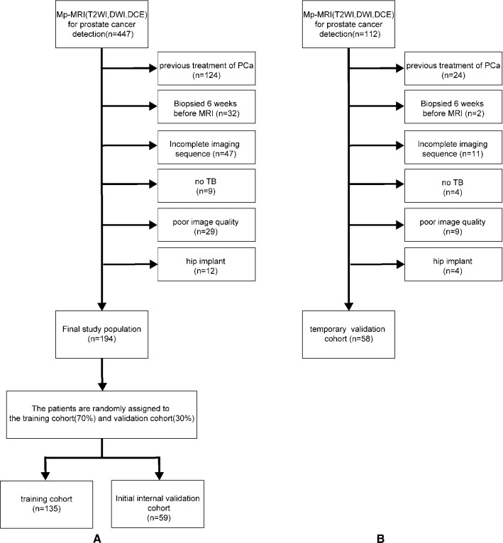
In this study, we performed retrospective modeling, internal validation and temporary validation. In the first part of retrospective modeling and internal validation, 447 patients who were enrolled from January 2014 to November 2018, with the following inclusion criteria: biopsy-naive status, clinical suspicion of PCa owing to either an elevated PSA level (> 4 ng/mL) or an abnormal DRE (digital rectal examination), complete mpMRI before biopsy, including target biopsy (TB) guided by mpMRI under the PI-RADS v1, v2 or v2.1 system and systemic biopsy in the same procedure. The exclusion criteria included the patients with any previous treatment of PCa, poor image quality or incomplete imaging sequence, marked artifact on MR images attributable to hip implant, or no TB. The selected patients were randomly divided into the training cohort (group 1, 70%, 135 patients) and the internal validation cohort (group 2, 30%, 59 patients). The patient selection is detailed in Fig. 1A.

Fig. 1.

Patient selection details in training cohort and internal validation cohort (A), temporal validation cohort (B). The horizontal arrow represents cases that meet the exclusion criteria to be removed from the study cohort

The above-mentioned inclusion and exclusion criteria were also used in the temporary validation. A total of 112 patients enrolled between January and November 2019 were selected according to the criteria for the temporary validation. The selected patients were assigned to the temporary validation cohort (group 3). Patients in group 3 did not belong to the same dataset as patients in group 1 and group 2 and were completely different in terms of the enrollment time and patient composition. The patient selection is detailed in Fig. 1B. The patient characteristics are detailed in Table 1.

Table 1.

Descriptive characteristics of the study population

Patient characteristics	Group 1 (n = 135)	Group 2 (n = 59)	Group 3 (n = 58)	P-Value
Age, years
Mean(± SD)  Median  Range  IQR	73.88(± 8.74) 75 50–93 69–80	76.62(± 7.9) 78 62–91 71–82.5	72.33(± 8.64) 73 53–90 66.25–78	group 1 vs 2:0.128 group 1 vs 3:0.273 group 2 vs 3:0.008
tPSA
Median  Range  IQR	18 0.35–300 8.23–57.5	22.9 4.56–300 11.5–91.3	15.3 0.22–159 6.96–32.92	group 1 vs 2:0.073 group 1 vs 3:0.182 group 2 vs 3:0.007
fPSA
Median  Range  IQR	2.5 0.04–25 1.17–6.265	2.73 0.3–25 1.65–10.75	1.82 0.01–25 1.01–4.99	group 1 vs 2:0.094 group 1 vs 3:0.184 group 2 vs 3:0.006
V
Median  Range  IQR	53.33 12.13–155.19 33.11–77.17	60.01 13.47–374.4 47.04–89.51	52.80 21.91–198.02 38.70–77.11	group 1 vs 2:0.038 group 1 vs 3:0.000 group 2 vs 3:0.000
PSAD
Median  Range  IQR	0.351 0.009–12.01 0.136–1.18	0.44 0.04–12.66 0.18–1.46	0.28 0.005–2.83 0.15–0.66	group 1 vs 2:0.343 group 1 vs 3:0.000 group 2 vs 3:0.000
csPC	53	22	18
ncsPC	82	37	40
GS
Grade group I  (GS0)  (GS4)  (GS5)  (GS6)	82(60.74%) 76(56.3%) 1(0.74%) 0(0%) 5(3.70%)	37(62.71%) 34(57.63%) 0(0%) 1(1.69%) 2(3.39%)	40(68.97%) 39(67.24%) 0(0%) 0(0%) 1(1.72%)	Percentage comparison: group 1 vs 2:0.998 group 1 vs 3:1 group 2 vs 3:1
Grade group II (GS 3 + 4 = 7)	11(8.15%)	7(11.86%)	4(6.90%)
Grade group III (GS 4 + 3 = 7)	8(5.93%)	0(0%)	4(6.90%)
Grade group IV (GS8)	6(4.44%)	5(8.47%)	6(10.34%)
Grade group V (GS9) (GS10)	28(20.74%) 20(14.81%) 8(5.93%)	10(16.95%) 9(15.25%) 1(1.69%)	4(6.90%) 3(5.17%) 1(1.72%)

group 1, Training cohort; group 2, internal validation cohort; group 3, temporary validation cohort; IQR, interquartile range; SD, standard deviation; tPSA, total prostate-specific antigen; fPSA, free prostate-specific antigen; V, volume of prostate measured on MRI; PSAD, prostate-specific antigen density; csPC, number of csPC; and ncsPC, number of ncsPC

Multiparametric MRI

All imaging was performed using a 1.5 T system (Magnetom Avanto, Siemens Healthcare) with a combined spine-array coil and a body-array receive-only coil (Tim Trio, Siemens Healthcare). None of the patients underwent bowel preparation or received butylscopolamine bromide. The scan sequences included high-resolution axial T2-weighted imaging, diffusion-weighted imaging (DWI) and DCE-MRI. The MRI parameters are listed in Supplementary Table S1.

Biopsy procedure and histopathologic examination

The standard 12-core systematic biopsy and TB were performed under the guidance of transrectal ultrasound (TRUS). Each core specimen was placed in a specific location of the prostate biopsy collection kits according to the prostate region that it came from. These biopsies included at least two additional cores for each target, and TB was recognized by cognitive registration based on the zonal anatomy or imaging landmarks, such that a urologist was needed to accurately associate real-time ultrasound images with the target lesions in the MRI images, and an experienced uroradiologist (6 years of experience in prostate MRI) helped the urologist to identify the details in and around the target lesion (prostate shape, verumontanum position, distance from the apex or the prostate base, presence of benign cyst or calcification nearby). The lesions with a GS ≥ 7 were defined as csPC.

ROI for image texture analysis and DCE-MRI quantitative analysis

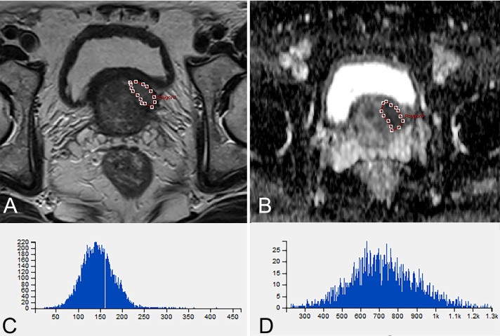
In the first part of modeling and internal validation, texture analysis (TA) was performed by one radiologist with 10 years of experience in prostate MRI, who assessed on the T2-weighted, diffusion-weighted and DCE MR images and independently performed TA using the Omni-Kinetics software (version 2.01, GE Healthcare). The regions of interest (ROIs) covering the entire tumor area were manually delineated on each axial slice based on the pathological results (Fig. 2). The ROIs of lesion layers were merged into a 3D ROI. The ROIs should be delineated on the main lesions, which were defined as the ones with the highest GS or most aggressive features [4]. Necrotic areas, cystic degeneration, hemorrhage, calcification, as well as the urethra, bladder, seminal vesicle and vascular nerve bundles should be as far as possible avoided. If a lesion turns out to be csPC, then it would be selected as a ROI. The areas with ncsPC, low-grade carcinoma, high-grade prostatic intraepithelial neoplasia or similarity to the manifestation of prostate cancer were defined as ROIs. For DCE-MRI, the extended Toft’s model (ETM) was implemented for the quantitative analysis of microcirculation.

Fig. 2.

A 66-year-old man with Gleason score 4 + 3 = 7 lesion. A T2-weighted MR image shows ROI of lesion (red) manually drawn for transition zone. B ADC mapping image shows ROI of lesion (red) manually drawn for transition zone. C Histogram of A. D Histogram of B

In the part of temporal validation, the ROIs were independently delineated by two radiologists (Doctor A: 10 years and Doctor B: 3 years of experience in prostate MRI) who were blind to the experiment following the above-described method, but without the pathological results to accord with when delineating.

Machine learning modeling and statistical analysis

The SPSSAU.com online tool was used for the statistical analyses of descriptive characteristics of the study population and the intra-class correlation (ICC) analysis of temporal validation. The other parts of the study, including modeling, validation, etc., were performed using the R language (version 3.63) programs. Feature extraction was also performed using the O.K. software. The types of the computer-derived features included first-order parameters, gradient-based histogram features, gray-level co-occurrence matrix (GLCM), run-length matrix (RLM), DCE-MRI quantitative features (extendedtofts_linear algorithm) and clinical parameters including the age, tPSA, fPSA, prostate volume and PSAD, which were calculated based on the voxels in the delineated ROIs (Supplementary Table S2). Although 233 features were extracted, not all of them were helpful in predicting csPC. Therefore, the R language programs were used to reduce the dimensionality, standardize the data and select the features. Logistic regression (LR), stepwise regression (SR), classical decision tree (cDT), conditional inference tree (CIT), random forest (RF) and support vector machine (SVM) models were constructed, and their diagnostic efficacy was compared with the receiver operating characteristic curve (ROC) and confounding matrix. Delong’s method was used to compare the difference in the area under the ROC curve (AUC), and a P < 0.05 was considered to be statistically significant. Finally, the models were validated using the data of the temporal validation group (n = 58), and the differences in the sensitivity, specificity, negative predictive value, positive predictive value and AUC of different models were compared.

Results

Patient characteristics

The ML modeling and internal validation included 194 male patients, while the temporal validation cohort included 58 male patients. The parameters of age, tPSA and fPSA significantly differed between groups 2 and 3. The volume of the prostate and PSAD significantly differed between groups 1 and 3, as well as between groups 2 and 3. There was no significant difference in the composition ratio of GS among the three groups (Table 1).

Model construction and internal validation evaluation

After dimensionality reduction and feature selection, the following eight independent variables were obtained: ADC.Quantile95, ADC.MinIntensity, ADC.uniformity, PSAD, T2.RelativeDeviation, Vp0.1, T2.Variance and T2.Quantile5 (Fig. 3) (Supplementary Table S3).

Fig. 3.

Counting from left to right on the horizontal axis, the solid blue dot is at the 8th position. It means that after dimension reduction and feature selection, eight independent variables were obtained. The X-axis represents the number of variables, and the Y-axis represents accuracy

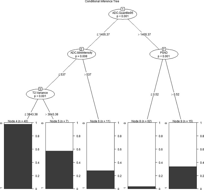
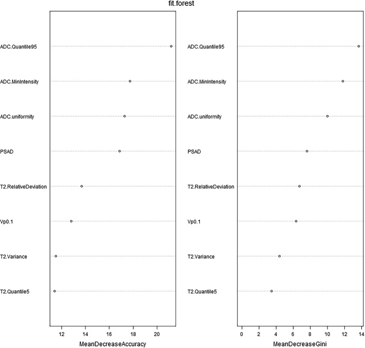
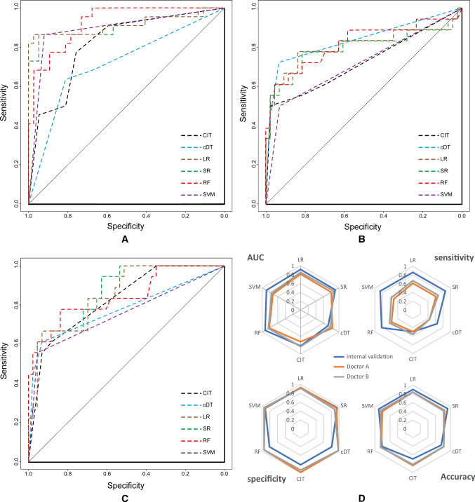
The independent predictors screened by the LR model were t2.Variance, ADC.Quantile95, Vp0.1 and ADC.MinIntensity (P < 0.05). The independent predictors of the SR model were T2.RelativeDeviation, ADC.MinIntensity, T2.Variance, ADC.Quantile95 and Vp0.1 (P < 0.05). In addition, the P values of ADC.Quantile95 and ADC.MinIntensity were less than 0.01. In the cDT model building, the cross-validation error and complexity parameter diagram are displayed in Fig. 4. The optimal tree was the tree divided twice (three terminal nodes) (Fig. 5). The CIT model is shown in Fig. 6, and the ordering of independent variables of the RF model according to importance is shown in Fig. 7. Figure 8 shows the ROC of the LR, SR, cDT, CIT, RF and SVM models in the internal validation cohort. Table 2 shows the diagnostic predictive features of the models of the internal validation cohort. The models with statistically significant differences in the AUC are displayed in Table 4. There were 7 cases with a GS = 7 in the internal validation cohort. Three cases were correctly classified by all ML models. Two cases were correctly classified by some of the ML models (DT, CIT misjudged twice; RF misjudged once). Two cases were misclassified by all ML models (Table S4).

Fig. 4.

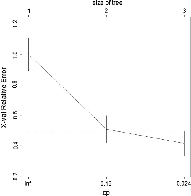
In cDT model building, the cross-validation error and complexity parameter diagram are displayed. The abscissa is the complexity parameter, and the ordinate is the cross-validation error. For all the trees with cross-validation errors within one standard deviation of the minimum cross-validation error, the tree with the lowest CP value is the optimal tree. The tree corresponding to the left-most CP value below the dotted line should be selected. The optimal tree is the tree divided twice (three terminal nodes)

Fig. 5.

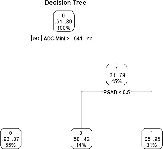
Classical decision tree model. The optimal tree was the tree divided twice (three terminal nodes). Start at the top of the tree, go down to the left if the condition is true, otherwise go down to the right, and the classification ends when the observation point reaches the terminal node. Each node has the probability of the corresponding category and the proportion of the sample

Fig. 6.

Conditional inference tree model. Start at the top of the tree, classify the two opposite conditions, one on the left and one on the right, and then classify more conditions. The shaded area in each node represents the corresponding csPC proportion, and the figure indicates the number of cases that meet the corresponding criteria

Fig. 7.

The importance ordering of independent variables of RF model is shown. MeanDecreaseAccuracy and MeanDecreaseGini indicate the importance of the variable. MeanDecreaseAccuracy: The degree to which the prediction accuracy of random forest decreases when the value of a variable is changed to a random number. The larger the value, the more important the variable. MeanDecreaseGini: The influence of each variable on the heterogeneity of observed values at each node of the classification tree was calculated to compare the importance of variables. The larger the value, the more important the variable

Fig. 8.

The ROC of LR, SR, cDT, CIT, RF and SVM models in the internal validation cohort are shown in A-C. AUC of ROC, sensitivity, specificity and accuracy for internal and temporal validation (two doctors) are shown on the radar chart in D. A-C: RF, LR and SR models have been relatively stable in the larger AUC during internal validation and temporal validation. In D, the blue line represents internal validation, and the orange and gray lines represent the ability of the machine learning model to classify the ROI delineated by the two radiologists. The orange line and gray line can be observed to almost coincide. The sensitivity of the machine learning model was reduced, but the AUC, specificity and accuracy were stable at a good level

Table 2.

Diagnostic predictive features of the models of the internal validation cohort

	Sensitivity	Specificity	PPV	NPV	Accuracy	AUC	YI
LR	0.86	0.92	0.86	0.92	0.9	0.915	0.78
SR	0.86	0.95	0.90	0.92	0.92	0.905	0.81
cDT	0.64	0.81	0.67	0.79	0.75	0.717	0.45
CIT	0.50	0.81	0.61	0.73	0.69	0.815	0.31
RF	0.82	0.81	0.72	0.88	0.81	0.925	0.63
SVM	0.86	0.92	0.86	0.92	0.9	0.891	0.78

PPV: positive predictive value; NPV: negative predictive value; and YI: Youden index

Table 4.

Models with statistically significant difference in AUC

Validations	Comparison of models	P
1. Internal validation
	RF VS. cDT	0.000
	CIT VS. cDT	0.04
	SVM VS. cDT	0.001
	SR VS. cDT	0.002
	LR VS. cDT	0.001
	RF VS. CIT	0.005
2. temporary validation
2.1 Doctor A
	cDT VS. SVM	0.027
2.2 Doctor A(GS 7 cases removed)
	RF VS. SVM	0.016
	SR VS. SVM	0.018
	LR VS. SVM	0.018
2.3 Doctor B
	CIT VS. SVM	0.041
	SR VS. SVM	0.018
	LR VS. SVM	0.031
	SR VS. DT	0.046
2.4 Doctor B(GS 7 cases removed)
	RF VS. CIT	0.048

Temporal validation evaluation

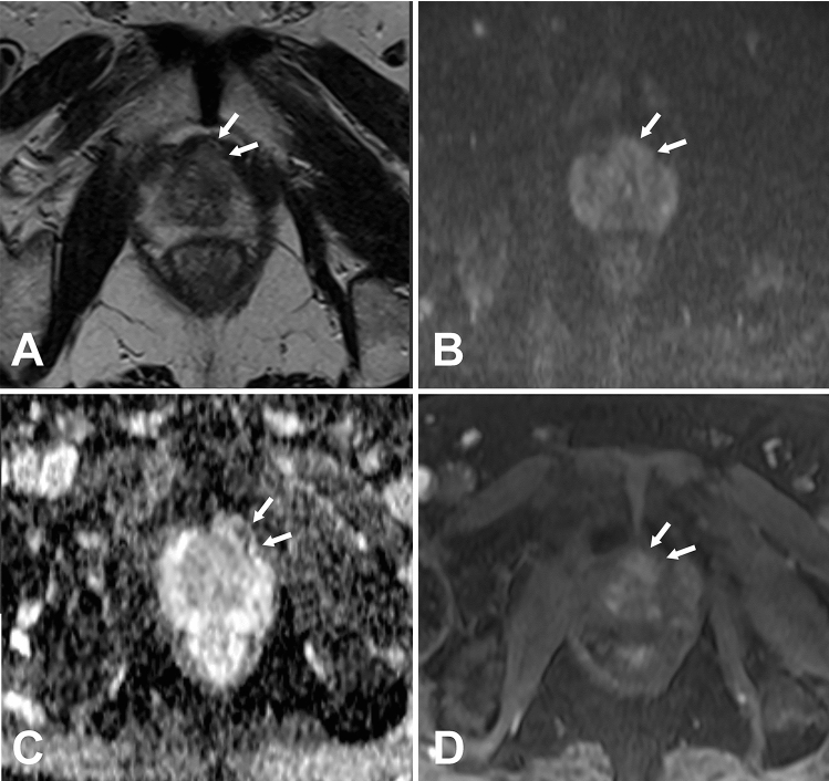
In the temporal validation, intra-class correlation (ICC) analysis was used to measure the degree of agreement across the raters on each of the 8 important variables. High concordance was found between the two observers in T2.RelativeDeviation, ADC.MinIntensity, T2.Quantile5 and ADC.uniformity, particularity in the last two, while a poor internal consistency was found in ADC.Quantile95, Vp0.1 and T2.Variance. The sensitivity of the temporal validation was lower than that of the internal validation (P < 0.05). The specificity, NPV, PPV, accuracy, AUC and YI of temporal validation were not significantly different from those of internal validation (P > 0.05). The classification ability of these models for GS > 7 cases was better than the cases with a GS = 7, and the classification performance remained stable for both GS > 7 and GS = 7 cases. There were 8 cases with a GS = 7 in the temporal validation cohort. Three cases were correctly classified by all ML models. Compared with the pathological results, the lesions with a PI-RADS score of 4–5 of these 3 cases could be found in the MR images (Fig. 2). The 5 cases that were misjudged by different models were the same (Table S4). In one case, the machine learning models misjudged 3 + 4 = 7 lesion (PI-RADS 4) in the transitional zone at the apex of the prostate. The lesion showed slightly low signal on T2WI, no significantly high signal on DWI (b = 800), uneven signal reduction on ADC and positive dynamic contrast enhancement with early enhancement (Fig. 9). No lesion of these 4 remaining cases with a PI-RADS score ≥ 3 could be found in the MR images (Fig. 10). When the cases with a GS of 7 were removed from the temporal validation database, the sensitivity and Youden index of all the models increased to varying degrees, as shown in Table 3. There was no change in the specificity of the models before and after removing the cases with a GS of 7, the PPV was slightly reduced, and the NPV was marginally increased.

Fig. 9.

A 78-year-old man, the machine learning models misjudged 3 + 4 = 7 lesion (PI-RADS 4) in the transitional zone at the apex of the prostate (white arrow). The lesion showed slightly low signal on T2WI, no significantly high sign on DWI (b = 800), uneven signal reduction on ADC and positive dynamic contrast enhancement with early enhancement

Fig. 10.

A 74-year-old man; only one core in the left TZa zone (No. 1 in A) had a GS of 4 + 3 = 7. The lesion accounted for 2% of the tissue strips, among which 4 score components accounted for 60% (1.8% of the tissue strips) and 3 score components accounted for 40% (0.8% of the tissue strips). The GS of the two cores from the right TZa and AFS (No. 3 and 2 in A, respectively) is 3 + 3 = 6, accounting for 4% and 1% of the tissue strips, respectively. No lesion with a PI-RADS score ≥ 3 could be found in the MR images, and the ML models misjudged

Table 3.

Comparison of the predictive features of the temporary validation

	Sensitivity/sensitivity *	Specificity/specificity *	PPV/PPV*	NPV/NPV*	Accuracy/Accuracy *	AUC/AUC*	YI/YI *
Doctor A
LR	0.61/0.89	0.93/0.93	0.79/0.73	0.85/0.98	0.84/0.92	0.81/0.97	0.54/0.82
SR	0.61/0.89	0.93/0.93	0.79/0.73	0.85/0.98	0.84/0.92	0.80/0.97	0.54/0.82
cDT	0.44/0.56	0.98/0.98	0.89/0.83	0.81/0.91	0.82/0.90	0.83/0.92	0.42/0.54
CIT	0.50/0.67	0.98/0.98	0.90/0.86	0.82/0.93	0.84/0.92	0.72/0.82	0.48/0.65
RF	0.56/0.78	0.95/0.95	0.83/0.78	0.84/0.95	0.84/0.92	0.82/0.96	0.51/0.73
SVM	0.50/0.67	0.93/0.93	0.75/0.67	0.82/0.93	0.8/0.88	0.72/0.80	0.43/0.6
Doctor B
LR	0.67/1	0.91/0.91	0.75/0.69	0.87/1	0.84/0.92	0.85/0.97	0.58/0.91
SR	0.67/1	0.88/0.88	0.71/0.64	0.86/1	0.82/0.9	0.86/0.97	0.55/0.88
cDT	0.44/0.56	0.98/0.98	0.89/0.83	0.81/0.91	0.82/0.9	0.78/0.92	0.42/0.54
CIT	0.56/0.78	0.93/0.93	0.77/0.7	0.83/0.95	0.82/0.9	0.83/0.92	0.49/0.71
RF	0.61/0.89	0.95/0.95	0.85/0.8	0.85/0.98	0.85/0.94	0.84/0.97	0.56/0.84
SVM	0.56/0.78	0.95/0.95	0.83/0.78	0.84/0.95	0.84/0.82	0.76/0.87	0.51/0.73

^*Gleason score 7 cases were removed

Discussion

In this study, mpMRI-TA, DCE-MRI quantitative analysis and clinical parameters were combined in a compound database. Eight important variables with the highest prediction accuracy were obtained after the feature selection and dimensionality reduction, and then, ML modeling and the evaluation of the models were carried out. According to Tables 3 and 4, the RF, LR and SR models have higher diagnostic abilities for csPC, and the overall performance of the SVM model in the temporal validation slightly declined. The performance of the RF, LR and SR models was relatively stable, not only in the unblinded internal validation, but also the blinded temporal validation, even though the number of experience years of the two doctors in the temporal validation greatly differed. Due to the existence of overfitting, prediction models may correspond too closely or accidentally be fitted to idiosyncrasies in the development dataset. In the three groups in this study, the differences in the baselines of some clinical parameters were statistically significant, but the classification ability of the machine learning models for different validation sets was still relatively stable, indicating that these models still had good universality when dealing with different datasets.

In the temporal validation, the sensitivity of each model was lower than that of the internal validation. The specificity, accuracy, PPV, NPV and AUC remained at a good level, similar to the internal validation. The analysis of the validations showed that the main misjudgments were in the cases with a GS of 3 + 4 = 7. When all the cases with a GS of 7 were removed from the database and verification was performed again, the sensitivity significantly increased to a level similar to that of internal validation. The reasons were analyzed as follows: (1) inherent differences between temporal and internal validation cohorts. Cases with 7 scores in the internal validation cohort accounted for 31.81% of csPC, while in the temporal validation cohort, cases with a score of 7 accounted for 44.44% of csPC, and the classification of cases with GS = 7 was difficult for ML-based classification. (2) Some lesions were too small. (3) Lesions are not typical on T2WI or DWI, and the corresponding texture data may not be adequate to be correctly classified by ML models. Our findings proved that ROI delineation is not the main cause of ML models misjudgment, since we repeated the experiment on 5 cases of misjudgment by ML models in the temporal verification group and the results remained unchanged. Small foci of the disease may be occult on mpMRI due to the limitations of the technology to resolve small nests of prostate cancer < 0.5 cc in volume, or due to a sparsely distributed tumor interspersed between the normal prostatic stroma [22, 23]. The study of Rozenberg et al. showed that the quantitative ADC measurements and individual ADC texture features had a limited performance in predicting GS upgrading of 3 + 4 = 7 cancers and identifying medium-risk tumors. Logistic regression models with several texture features can improve the prediction accuracy [24]. Further studies are needed to evaluate the ability of ADC texture analysis to identify moderate-risk tumors. Considering the active surveillance, the proportion of GS 3 + 4 = 7 tumors may be one of the important factors. Since the long-term prognosis of GS 3 + 4 = 7 tumors is significantly different from that of GS 4 + 3 = 7 prostate cancer, it is increasingly important to distinguish between the two types of tumors with different GS [25].

The RF model is a classifier that contains multiple decision trees. RF has shown an excellent classification performance for processing balanced sample sets, with few adjustment parameters and good noise tolerance. Besides, it is not prone to overfitting and can efficiently process a large number of features [26]. Nathan Lay et al. established an RF model and an SVM model based on MRI signals and texture features. Their results showed that the RF model with an AUC of 0.93 was superior to the SVM model with an AUC of 0.86 [27], which is basically consistent with the corresponding results of our study. SVM has shown a high performance in processing data that are nonlinear or have a small number of samples or high dimensions [28]. SVM classifiers developed in combination with the PI-RADS scores and MR radiomics features have made significant advances in the diagnosis of prostate cancer in several recent studies [29]. In this study, SVM classifiers performed well in the internal validation, but had a slightly lower performance in the temporal validation. LR is one of the most commonly used ML algorithms in dichotomous tasks. It is a supervised learning ML algorithm that is widely used due to its ease of use and interpretability [30]. Some predictive variables based on LR that do not pass the significance test are removed, and then, the SR model is obtained. In our study, since the database was selected for dimensionality reduction and feature selection in advance, only a few variables with a high prediction accuracy were retained. The results of our study showed that there was no significant difference in the diagnostic efficiency between the LR and SR models. The cDT model is a common model for data mining, which is based on binary output variables and a set of predictive variables. CIT is a variant of cDT, but the variable selection and ROI delineations are based on significance tests rather than intra-group homogeneity. The cDT was built using the rpart software package, and CIT was built using the Party package and does not require pruning. The threshold determines the complexity of the model. Decision tree models are prone to overfitting [31], but RF models basically avoid this problem.

In this study, the RF model ranked the parameters according to their importance, and the top five items in the charts of MeanDecreaseAccuracy and MeanDecreaseGini were ADC.Quantile95, ADC.MinIntensity, ADC.uniformity, PSAD and T2.RelativeDeviation. The first three parameters are all related to the ADC texture analysis. PSAD is a derived parameter of PSA that represents the PSA content of the prostate per unit volume. It has already been shown that the diagnostic accuracy can be increased by adding the PSA density levels to the diagnostic process [3, 32]. Adding the parameters of age and PSA density to the PI-RADS scores improves the diagnostic accuracy for csPCa. A combination of these variables with PI-RADS v2 can help to avoid unnecessary in-bore biopsies while still detecting the majority of csPC lesions [33]. The T2WI relative texture parameter T2.RelativeDeviation was ranked 5th in the importance ranking, while Vp0.1, a parameter derived from the DCE-MRI quantitative analysis, was ranked 6th. Vp represents the percentage of the intravascular contrast medium volume, reflecting the characteristics of the increased average vascular density, increased perfusion vessels and high vascular permeability.

This study has some limitations as follows. First, since the sample size was relatively small, the convolutional neural network model was not selected for evaluation. Second, part of the pathological results came from the ultrasound-guided puncture biopsy, which could not avoid the possibility of missed puncture diagnosis. Third, no specific study has been specifically performed for a large number of cases with a GS of 7, which will be covered in the next study. Fourthly, manual segmentation was adopted in this study, and 3D automatic segmentation with higher efficiency based on deep learning of csPC will be performed in the following study [34].

Conclusions

Machine learning models have a good classification ability for csPC. Compared with internal validation, the sensitivity of each model in temporal validation was reduced, but the specificity, accuracy and area under the ROC curve remained stable at a good level. The RF, LR and SR models have a better classification performance in imaging-based diagnosis of csPC, and ADC texture-related parameters are among the parameters with the highest importance.

Supplementary Information

Below is the link to the electronic supplementary material.

Authors’ contributions

Tao Peng carried out the conception and design, revised the manuscript and approved the final version to be published. XiangKe Niu carried out conception and design and approved the final version to be published. JianMing Xiao and ChaoBang Gao participated in the conception and design, drafted and revised the manuscript and analyzed and interpreted the data. Lin Li, Bingjie Pu, Xiaohui Zeng and Zongyong Wang participated in the design of the study and performed the statistical analysis. Ci Li, Lin Chen and Jin Yang conceived of the study, participated in its design and coordination and helped to revise the manuscript. Tao Peng and Lin Li contributed to acquisition of data, analysis and interpretation of data.

Funding

The study was funded by Health and Family Planning Commission of Sichuan Province (Grant 18PJ150, recipient Tao Peng, and Grant 17PJ430, recipient XiangKe Niu) and Chengdu (Sichuan, China) (Grant 2018055, recipient ZongYong Wang, and Grant 2021036, recipient Tao Peng).

Availability of data and material

The data that support the findings of this study are available from the corresponding author on reasonable request.

Code availability

The custom code of this study is available from the corresponding author on reasonable request.

Declarations

Conflict of interest

The authors declare that they have no known competing financial interests or personal relationships that could have appeared to influence the work reported in this paper. Tao Peng declared that they had no competing interests. JianMing Xiao declared that they had no competing interests. Lin Li declared that they had no competing interests. BingJie Pu declared that they had no competing interests. XiangKe Niu declared that they had no competing interests. XiaoHui Zeng declared that they had no competing interests. ZongYong Wang declared that they had no competing interests. ChaoBang Gao declared that they had no competing interests. Ci Li declared that they had no competing interests. Lin Chen declared that they had no competing interests. Jin Yang declared that they had no competing interests.

Ethical approval

The study has been approved by the Institutional Review Board (IRB) of our institute, and patient consent form was waived because this is a retrospective study with anonymized data.

Consent to participate

Not applicable.

Consent for publication

Not applicable.

References

- 1.Bray F, Ferlay J, Soerjomataram I, Siegel RL, Torre LA, Jemal A. Global cancer statistics 2018: GLOBOCAN estimates of incidence and mortality worldwide for 36 cancers in 185 countries. CA Cancer J Clin. 2018;68(6):394–424. doi: 10.3322/caac.21492. [DOI] [PubMed] [Google Scholar]
- 2.Center MM, Jemal A, Lortet-Tieulent J, Ward E, Ferlay J, Brawley O, Bray F. International variation in prostate cancer incidence and mortality rates. Eur Urol. 2012;61(6):1079–1092. doi: 10.1016/j.eururo.2012.02.054. [DOI] [PubMed] [Google Scholar]
- 3.Friedl A, Schneeweiss J, Sevcenco S, Eredics K, Kunit T, Susani M, Kivaranovic D, Eisenhuber-Stadler E, Lusuardi L, Brossner C, Schima W. In-bore 3.0-T magnetic resonance imaging-guided transrectal targeted prostate biopsy in a repeat biopsy population: diagnostic performance, complications, and learning curve. Urology. 2018;114:139–146. doi: 10.1016/j.urology.2017.12.032. [DOI] [PubMed] [Google Scholar]
- 4.Weinreb JC, Barentsz JO, Choyke PL, Cornud F, Haider MA, Macura KJ, Margolis D, Schnall MD, Shtern F, Tempany CM, Thoeny HC, Verma S. PI-RADS prostate imaging-reporting and data system: 2015, version 2. Eur Urol. 2016;69(1):16–40. doi: 10.1016/j.eururo.2015.08.052. [DOI] [PMC free article] [PubMed] [Google Scholar]
- 5.Chen R, Ren S, Chinese Prostate Cancer C, Yiu MK, Fai NC, Cheng WS, Ian LH, Naito S, Matsuda T, Kehinde E, Kural A, Chiu JY, Umbas R, Wei Q, Shi X, Zhou L, Huang J, Huang Y, Xie L, Ma L, Yin C, Xu D, Xu K, Ye Z, Liu C, Ye D, Gao X, Fu Q, Hou J, Yuan J, He D, Pan T, Ding Q, Jin F, Shi B, Wang G, Liu X, Wang D, Shen Z, Kong X, Xu W, Deng Y, Xia H, Cohen AN, Gao X, Xu C, Sun Y (2014) Prostate cancer in Asia: A collaborative report. Asian J Urol 1(1):15-29 [DOI] [PMC free article] [PubMed]
- 6.Albertsen PC, Hanley JA, Fine J. 20-year outcomes following conservative management of clinically localized prostate cancer. JAMA. 2005;293(17):2095–2101. doi: 10.1001/jama.293.17.2095. [DOI] [PubMed] [Google Scholar]
- 7.Sanda MG, Cadeddu JA, Kirkby E, Chen RC, Crispino T, Fontanarosa J, Freedland SJ, Greene K, Klotz LH, Makarov DV, Nelson JB, Rodrigues G, Sandler HM, Taplin ME, Treadwell JR. Clinically localized prostate cancer: AUA/ASTRO/SUO Guideline. Part I: risk stratification, shared decision making, and care options. J Urol. 2018;199(3):683–690. doi: 10.1016/j.juro.2017.11.095. [DOI] [PubMed] [Google Scholar]
- 8.Chatterjee A, Harmath C, Oto A (2020) New prostate MRI techniques and sequences. Abdom Radiol NY [DOI] [PubMed]
- 9.Turkbey B, Rosenkrantz AB, Haider MA, Padhani AR, Villeirs G, Macura KJ, Tempany CM, Choyke PL, Cornud F, Margolis DJ, Thoeny HC, Verma S, Barentsz J, Weinreb JC. Prostate imaging reporting and data system version 2.1: 2019 Update of prostate imaging reporting and data system version 2. Eur Urol. 2019;76(3):340–351. doi: 10.1016/j.eururo.2019.02.033. [DOI] [PubMed] [Google Scholar]
- 10.Giambelluca D, Cannella R, Vernuccio F, Comelli A, Pavone A, Salvaggio L, Galia M, Midiri M, Lagalla R, Salvaggio G (2019) PI-RADS 3 Lesions: role of prostate MRI texture analysis in the identification of prostate cancer. Curr Probl Diagn Radiol [DOI] [PubMed]
- 11.Rosenkrantz AB, Oto A, Turkbey B, Westphalen AC. Prostate imaging reporting and data system (PI-RADS), version 2: A critical look. AJR Am J Roentgenol. 2016;206(6):1179–1183. doi: 10.2214/AJR.15.15765. [DOI] [PubMed] [Google Scholar]
- 12.Borofsky S, George AK, Gaur S, Bernardo M, Greer MD, Mertan FV, Taffel M, Moreno V, Merino MJ, Wood BJ, Pinto PA, Choyke PL, Turkbey B. What are we missing? False-negative cancers at multiparametric MR imaging of the prostate. Radiology. 2018;286(1):186–195. doi: 10.1148/radiol.2017152877. [DOI] [PMC free article] [PubMed] [Google Scholar]
- 13.Futterer JJ, Briganti A, De Visschere P, Emberton M, Giannarini G, Kirkham A, Taneja SS, Thoeny H, Villeirs G, Villers A. Can clinically significant prostate cancer be detected with multiparametric magnetic resonance imaging? A systematic review of the literature. Eur Urol. 2015;68(6):1045–1053. doi: 10.1016/j.eururo.2015.01.013. [DOI] [PubMed] [Google Scholar]
- 14.Niaf E, Lartizien C, Bratan F, Roche L, Rabilloud M, Mege-Lechevallier F, Rouviere O. Prostate focal peripheral zone lesions: characterization at multiparametric MR imaging–influence of a computer-aided diagnosis system. Radiology. 2014;271(3):761–769. doi: 10.1148/radiol.14130448. [DOI] [PubMed] [Google Scholar]
- 15.Niu XK, Chen ZF, Chen L, Li J, Peng T, Li X. Clinical application of biparametric MRI texture analysis for detection and evaluation of high-grade prostate cancer in zone-specific regions. AJR Am J Roentgenol. 2018;210(3):549–556. doi: 10.2214/AJR.17.18494. [DOI] [PubMed] [Google Scholar]
- 16.Jovic S, Miljkovic M, Ivanovic M, Saranovic M, Arsic M. Prostate cancer probability prediction by machine learning technique. Cancer Invest. 2017;35(10):647–651. doi: 10.1080/07357907.2017.1406496. [DOI] [PubMed] [Google Scholar]
- 17.Li M, Chen T, Zhao W, Wei C, Li X, Duan S, Ji L, Lu Z, Shen J. Radiomics prediction model for the improved diagnosis of clinically significant prostate cancer on biparametric MRI. Quant Imaging Med Surg. 2020;10(2):368–379. doi: 10.21037/qims.2019.12.06. [DOI] [PMC free article] [PubMed] [Google Scholar]
- 18.Bonekamp D, Kohl S, Wiesenfarth M, Schelb P, Radtke JP, Gotz M, Kickingereder P, Yaqubi K, Hitthaler B, Gahlert N, Kuder TA, Deister F, Freitag M, Hohenfellner M, Hadaschik BA, Schlemmer HP, Maier-Hein KH. Radiomic machine learning for characterization of prostate lesions with MRI: comparison to ADC values. Radiology. 2018;289(1):128–137. doi: 10.1148/radiol.2018173064. [DOI] [PubMed] [Google Scholar]
- 19.Vernuccio F, Cannella R, Comelli A, Salvaggio G, Lagalla R, Midiri M. Radiomics and artificial intelligence: new frontiers in medicine. Recenti Prog Med. 2020;111(3):130–135. doi: 10.1701/3315.32853. [DOI] [PubMed] [Google Scholar]
- 20.Ramspek CL, Jager KJ, Dekker FW, Zoccali C, van Diepen M. External validation of prognostic models: what, why, how, when and where? Clin Kidney J. 2021;14(1):49–58. doi: 10.1093/ckj/sfaa188. [DOI] [PMC free article] [PubMed] [Google Scholar]
- 21.Siontis GC, Tzoulaki I, Castaldi PJ, Ioannidis JP. External validation of new risk prediction models is infrequent and reveals worse prognostic discrimination. J Clin Epidemiol. 2015;68(1):25–34. doi: 10.1016/j.jclinepi.2014.09.007. [DOI] [PubMed] [Google Scholar]
- 22.Tsai WC, Field L, Stewart S, Schultz M. Review of the accuracy of multi-parametric MRI prostate in detecting prostate cancer within a local reporting service. J Med Imaging Radiat Oncol. 2020;64(3):379–384. doi: 10.1111/1754-9485.13029. [DOI] [PubMed] [Google Scholar]
- 23.Schoots IG. MRI in early prostate cancer detection: how to manage indeterminate or equivocal PI-RADS 3 lesions? Transl Androl Urol. 2018;7(1):70–82. doi: 10.21037/tau.2017.12.31. [DOI] [PMC free article] [PubMed] [Google Scholar]
- 24.Rozenberg R, Thornhill RE, Flood TA, Hakim SW, Lim C, Schieda N. Whole-tumor quantitative apparent diffusion coefficient histogram and texture analysis to predict gleason score upgrading in intermediate-risk 3 + 4 = 7 prostate cancer. AJR Am J Roentgenol. 2016;206(4):775–782. doi: 10.2214/AJR.15.15462. [DOI] [PubMed] [Google Scholar]
- 25.Epstein JI, Zelefsky MJ, Sjoberg DD, Nelson JB, Egevad L, Magi-Galluzzi C, Vickers AJ, Parwani AV, Reuter VE, Fine SW, Eastham JA, Wiklund P, Han M, Reddy CA, Ciezki JP, Nyberg T, Klein EA. A contemporary prostate cancer grading system: a validated alternative to the gleason score. Eur Urol. 2016;69(3):428–435. doi: 10.1016/j.eururo.2015.06.046. [DOI] [PMC free article] [PubMed] [Google Scholar]
- 26.Qian C, Wang L, Gao Y, Yousuf A, Yang X, Oto A, Shen D. In vivo MRI based prostate cancer localization with random forests and auto-context model. Comput Med Imaging Graph. 2016;52:44–57. doi: 10.1016/j.compmedimag.2016.02.001. [DOI] [PMC free article] [PubMed] [Google Scholar]
- 27.Lay N, Tsehay Y, Greer MD, Turkbey B, Kwak JT, Choyke PL, Pinto P, Wood BJ, Summers RM. Detection of prostate cancer in multiparametric MRI using random forest with instance weighting. J Med Imaging (Bellingham) 2017;4(2):024506. doi: 10.1117/1.JMI.4.2.024506. [DOI] [PMC free article] [PubMed] [Google Scholar]
- 28.Fasshauer GE, Hickernell FJ, Ye Q. Solving support vector machines in reproducing kernel Banach spaces with positive definite functions. Appl Comput Harmon Anal. 2015;38(1):115–139. doi: 10.1016/j.acha.2014.03.007. [DOI] [Google Scholar]
- 29.Wang J, Wu C-J, Bao M-L, Zhang J, Wang X-N, Zhang Y-D. Machine learning-based analysis of MR radiomics can help to improve the diagnostic performance of PI-RADS v2 in clinically relevant prostate cancer. Eur Radiol. 2017;27(10):4082–4090. doi: 10.1007/s00330-017-4800-5. [DOI] [PubMed] [Google Scholar]
- 30.Eftekhar B, Mohammad K, Ardebili HE, Ghodsi M, Ketabchi E (2005) Comparison of artificial neural network and logistic regression models for prediction of mortality in head trauma based on initial clinical data. BMC Medical Informatics and Decision Making, 5(1) [DOI] [PMC free article] [PubMed]
- 31.Tong W, Xie Q, Hong H, Fang H, Shi L, Perkins R, Petricoin EF. Using decision forest to classify prostate cancer samples on the basis of SELDI-TOF MS data: assessing chance correlation and prediction confidence. Environ Health Perspect. 2004;112(16):1622–1627. doi: 10.1289/txg.7109. [DOI] [PMC free article] [PubMed] [Google Scholar]
- 32.Brizmohun Appayya M, Sidhu HS, Dikaios N, Johnston EW, Simmons LA, Freeman A, Kirkham AP, Ahmed HU, Punwani S. Characterizing indeterminate (Likert-score 3/5) peripheral zone prostate lesions with PSA density, PI-RADS scoring and qualitative descriptors on multiparametric MRI. Br J Radiol. 2018;91(1083):20170645. doi: 10.1259/bjr.20170645. [DOI] [PMC free article] [PubMed] [Google Scholar]
- 33.Polanec SH, Bickel H, Wengert GJ, Arnoldner M, Clauser P, Susani M, Shariat SF, Pinker K, Helbich TH, Baltzer PAT. Can the addition of clinical information improve the accuracy of PI-RADS version 2 for the diagnosis of clinically significant prostate cancer in positive MRI? Clin Radiol. 2020;75(2):e151–e157. doi: 10.1016/j.crad.2019.09.139. [DOI] [PubMed] [Google Scholar]
- 34.Comelli A, Dahiya N, Stefano A, Vernuccio F, Portoghese M, Cutaia G, Bruno A, Salvaggio G, Yezzi A (2021) Deep learning-based methods for prostate segmentation in magnetic resonance imaging. Appl Sci (Basel) 11(2) [DOI] [PMC free article] [PubMed]
Associated Data
This section collects any data citations, data availability statements, or supplementary materials included in this article.
Supplementary Materials
Data Availability Statement