

Abstract
Continuous treatments propensity scoring remains understudied as the majority of methods are focused on the binary treatment setting. Current propensity score methods for continuous treatments typically rely on weighting in order to produce causal estimates. It has been shown that in some continuous treatment settings, weighting methods can result in worse covariate balance than had no adjustments been made to the data. Furthermore, weighting is not always stable, and resultant estimates may be unreliable due to extreme weights. These issues motivate the current development of novel propensity score stratification techniques to be used with continuous treatments. Specifically, the generalized propensity score cumulative distribution function (GPS-CDF) and the nonparametric GPS-CDF (npGPS-CDF) approaches are introduced. Empirical CDFs are used to stratify subjects based on pretreatment confounders in order to produce causal estimates. A detailed simulation study shows superiority of these new stratification methods based on the empirical CDF, when compared to standard weighting techniques. The proposed methods are applied to the “Mexican American Tobacco use in Children” (MATCh) study to determine the causal relationship between continuous exposure to smoking imagery in movies, and smoking behavior among Mexican-American adolescents. These promising results provide investigators with new options for implementing continuous treatment propensity scoring.
Keywords: Causal Inference, Continuous Treatment, Observational Study, Propensity Score, Smoking Initiation
1. Introduction
Propensity scoring is often used to make causal inference about a treatment/exposure-outcome relationship in non-randomized observational studies, when assumptions are met (unconfoundedness, consistency, positivity, and no misspecification of the propensity score model).1-3 Propensity score methods are commonly applied in settings with continuous outcomes. More recently, binary outcomes, which are common in clinical research, have been investigated with a focus on reporting odds ratios (ORs).4-6 These causal OR estimates (i.e., marginal odds ratios) can be derived using logistic regression techniques that do not adjust for additional covariates.4-6
Although methods for binary and more recently, multiple treatments have been well-studied,7-13 there has been less research devoted to propensity score methods for continuous treatments, and no studies to our knowledge have investigated estimation of marginal odds ratios with continuous treatments. In this paper, continuous treatments refer to treatment assignment (e.g. dosing trials) or continuous exposures (e.g. environmental exposures). In the presence of continuous treatments, investigators sometimes dichotomize or categorize the treatment in order to utilize more well-established propensity score techniques.14-17 However, it has been shown that categorization of a continuous treatment may lead to loss of information and subsequent decrease in power when conducting outcome analyses.18,19 Also, not analyzing exposures on their original scale may produce clinical interpretations that are awkward to domain-area researchers.
Propensity score methods directly applicable to continuous exposures have been proposed. For example, maximum likelihood estimates (MLEs) derived from linear models have been used to estimate the generalized propensity score (GPS).1,7,20 Within the continuous treatment framework, r(t,x) is defined as the conditional density of the treatment given the baseline covariates,
| (1) |
It then follows that the GPS is defined as R = r(T,X).1 This GPS has a balancing property such that within strata with the same value for r(t,X), the probability that T = t does not depend on X.1 It follows from this formulation that treatment assignment is unconfounded given the GPS. More details on the full derivation and balancing properties of the GPS within the continuous treatment setting are given by Hirano and Imbens.1
In practice, the GPS can be obtained by fitting a linear regression model of the form
| (2) |
where T is a continuous treatment, X is a vector of potential confounders, and ε ~ N(0, σ2). The GPS for individual i, is then estimated as,
| (3) |
where Ti is the true value of the continuous treatment for subject i, is the subject specific predicted treatment from equation (2), and is the estimated variance of the regression model. The estimated GPS, , may then be applied directly via regression adjustment or with inverse probability weighting (IPW) in order to produce causal treatment estimates.1,18,20-25 Hirano et. al first proposed implementation of the estimated GPS, , through direct covariate adjustment.1 Covariate adjustment using the GPS involves regressing the outcome on both the continuous treatment and the GPS, using a flexible function of the treatment and GPS (i.e. quadratic approximation).1 Simulations have shown that implementation of the GPS via covariate adjustment results in causal estimates that are sensitive to model misspecification.26,27 Although methods that utilize machine learning algorithms, e.g. the Super Learner, have been developed to mitigate the effects of model misspecification when performing covariate adjustment using the GPS, their performance has not been well-tested via simulation;25 these methods are therefore not the focus of the current study.
Robins et al. propose implementing the GPS to produce causal estimates using IPW.20 Briefly, IPW weights each individual by the inverse of the density function evaluated at the observed treatment value. Specifically, in the calculation of , subjects with unexpected covariate distributions will have large estimates for , and conversely will have small values for . Thus, the IPW, given by
| (4) |
will be higher, effectively giving more weight to subjects that have unexpected covariate distributions based on their continuous treatment level. By up-weighting those individuals less likely to receive the treatment, IPW gives more weight in the analysis to subjects with dissimilar covariate distributions than subjects with similar covariate profiles (i.e. subject specific covariate values) within the same treatment level. Weights of the above form may be too large, so a stabilizing factor is applied to wi in practice.20 This stabilizing factor, W(Ti), is given by the marginal density of T, which may be estimated by first fitting an intercept only model of the form
| (5) |
where . The stabilizing factor is estimated as
| (6) |
where is the mean treatment value of the sample.21 The final estimated stabilized IPW is given by
| (7) |
These weights may then be applied in a weighted outcome regression in order to estimate a causal treatment effect.23
Although the calculation of these weights is straightforward, this MLE method relies heavily on correctly specifying the linear treatment model.20,22,23 If the model is not correctly specified or the model assumptions are not met (e.g., deviations from normality of errors), it has been shown that the MLE method can produce extreme weights that can lead to severely biased causal inference estimates.18 Therefore, methods that operate outside of the MLE framework may produce better weights, resulting in more covariate balance, and less biased estimates of the outcome.
Nonparametric methods of estimating the GPS vector have been shown to provide more accurate estimates of the GPS compared to parametric regression.24,28 One such method that has gathered traction is the generalized boosted model (GBM).18,24 GBM fits a general model of the form,
| (8) |
where ε ~ N(0, σ2) and m(X) is the mean function of T given X.24 The mean function is estimated using a boosting algorithm that additively fits regression trees until the model is sufficiently flexible to fit the data.24,29 With the mean function derived, stabilized IPWs can be calculated and implemented just as in the MLE weighting procedure. Although it may appear as though GBM ultimately provides minimally biased causal inference estimates, there are still drawbacks that limit its usefulness. First, GBM does not afford users the ability to force variables into the final treatment model,30 which is often appropriate in biomedical research (for example, age, gender, and other demographic or baseline clinical information). Additionally, although GBM has been shown to outperform MLE in simulation studies, covariate balance after GBM weighting can still remain poor, subsequently resulting in more unstable estimates than if weights were not applied at all.18 Finally, the primary way to improve balance using GBM is by increasing the number of regression trees used by the method, which may not provide adequate control over sample imbalance.18
Recent important extensions of the “covariate balancing propensity score,” which models treatment assignment while optimizing covariate balance, have been made for continuous treatments.18,31 Specifically, the new covariate balancing generalized propensity score (CBGPS) uses the method of moments framework to derive IPWs such that the weighted correlation between X and T is minimized.18 Furthermore, the nonparametric extension of this CBGPS (npCBGPS) places no parametric restrictions on the GPS, as weights are directly derived without giving a functional form to the propensity scores.18
Although the CBGPS is a method for optimizing covariate balance while estimating the GPS, it is not without limitations as shown in Fong et al.18 In simulations, it was shown that GBM produces less biased causal estimates compared to CBGPS and npCBGPS when sample sizes are large (~1,000). Additionally, since the nonparametric extension, npCBGPS, is based on an empirical likelihood approach, there is no guarantee that the optimization procedures find the global optimum. Furthermore, when the number of covariates is large, or if X strongly predicts T, npCBGPS may fail to find a solution, leaving the investigator to sacrifice covariate balance to derive weights. Moreover, even in scenarios where the CBGPS and npCBGPS methods produce the best covariate balance, they may not produce causal inference estimates with the lowest bias.
In sum, methods for creating balanced data in the continuous treatment setting have relied heavily on weighting procedures. Although nonparametric methods have been proposed to derive weights, it has been well-studied that weighting methods may produce unreliable causal inference estimates due to extreme weights.18,24 The current literature indicates alternatives to weighting are desirable in some settings. Therefore, this paper seeks to derive stratification methods that neither utilize weighting nor rely on parametric assumptions in order to produce more reliable causal inference estimates with continuous treatments. Specifically, the current paper proposes two novel methodologies that produce causal estimates for continuous treatments: both the generalized propensity score cumulative distribution function (GPS-CDF) and the nonparametric GPS-CDF (npGPS-CDF) methods stratify subjects, based on pretreatment covariate distributions, in order to produce causal estimates.
2. Methods
Stratifying subjects with the objective of achieving covariate balance based on pretreatment confounders amounts to creating groups of subjects with similar covariate distributions who received different treatments. With this goal in mind, this section describes two novel stratification methods that seek to refine current methods in order to produce better covariate balance and more accurate causal treatment effect estimates. Both proposed methods create subject specific covariate distributions that are used in order to create balancing strata.
2.1. GPS-CDF - parametric approach
The GPS-CDF approach creates balancing strata from a regression model in order to produce causal treatment effect estimates. However, to improve balance, a representation of the distribution of an individual’s covariates is proposed, rather than using just the observed instance. This distribution, which is derived through bootstrapping, provides detailed covariate information for each subject. While it is possible to group subjects based only on the predicted values produced from an initial regression model, there exists a possibility of subjects with similar initial predicted values presenting with different covariate distributions. This will especially be true when the regression model does not fit well to the data.
The bootstrapping algorithm of the GPS-CDF method begins by fitting any regression model in the form of equation (2), that returns model estimates, in order to predict the continuous treatment (e.g., generalized linear model). , or a subject’s predicted treatment, is calculated by multiplying the estimated model coefficients by each subject’s covariate profile,
| (9) |
To further capture the complete covariate profile of a subject, B sets of coefficients are resampled assuming a multivariate normal distribution,
| (10) |
where b = 1, … , B, and and are the estimated mean vector and variance matrix, respectively, derived from the original treatment regression model where B is an arbitrarily large number (taken in this paper to be 10,000). The is then calculated for each subject using each of the B sets of sampled coefficients,
| (11) |
for b = 1, … , B. The full set of represents a bootstrapped distribution of each subject’s predicted treatment values. Each subject specific distribution () may be thought of as a separate unimodal density that fully encapsulates the effect of the covariate profile on the treatment for each subject.
As is derived through variation in , two subjects with identical covariate profiles (Xi) will have identical , and similarly, subjects with identical will have identical covariate profiles, as long as the GPS model in equation (2) is identifiable. Therefore, subjects with similar will have, on average, similar covariate distributions. Thus, a function that accurately maps for each subject can subsequently be used to classify subjects into covariate balancing strata.
Next, an empirical cumulative density function (eCDF) is estimated in the natural way:
| (12) |
where I is the indicator function. The shape of the eCDF for each subject is a strictly non-decreasing function. Furthermore, as the eCDF is a 1-to-1 function of , subjects with similar eCDFs will have similar , and resultantly, similar covariate distributions. One proposed equation used to map the eCDF is a 2-parameter logistic curve given by,
| (13) |
where si represents the subject specific scale parameter of the logistic curve, and μi is the subject specific location parameter. Once eCDFs are calculated for each subject, a non-linear least squares (NLS) algorithm,32 given by equation (14), is used to fit the logistic curve.
| (14) |
The above NLS algorithm iteratively fits values for si and μi, for each subject, until the residual distance between the eCDF and fitted logistic curve is minimized.32,33 Based on the fitted logistic curve, subjects with similar values for si and μi will have similar eCDF vectors and thus similar covariate distributions. Each individual’s si and μi value can then be used to group subjects with similar covariate profiles. Although there are many ways to classify subjects into strata based on two variables, k-Means clustering (KMC) has been shown to provide the highest covariate similarity within clusters.34 Additionally, while any number of strata can be formed, following the convention set within binary treatment propensity score analyses, 5 strata are created.11,35-37 Thus using KMC, subjects can be accurately placed into one of five strata with subjects with similar values for both si and μi, and subsequently similar covariate distributions.
Once all subjects have been assigned covariate balancing strata, treatment effect estimates are estimated using outcome analyses which account for stratification (e.g. conditional logistic regression). Additionally, as variation arises from estimating the GPS, bootstrapping may be utilized in order to find valid estimates of the treatment effect standard error, a common practice within propensity score methods.18,38,39 Further details of the bootstrapping procedure to produce confidence intervals for treatment effect estimates may be found in Austin et al. and Fong et al.18,38 and a practical example of the bootstrapping procedure is presented here in Section 5. The following steps detail the GPS-CDF stratification procedure:
Choose variables related to the treatment to include in the treatment model (see Brookhart et al. for a detailed discussion of variable selection for propensity models).40
Fit a regression model to predict the continuous treatment (e.g. generalized linear model).
Retain the treatment regression model estimates, and .
Resample B sets of coefficients assuming a multivariate normal distribution based on and .
Calculate for each subject using each set of sampled coefficients.
Calculate an eCDF, across the set of , for each subject.
Fit a 2-parameter logistic curve to each subject specific eCDF to obtain si and μi.
Use KMC to create five balancing strata based on si and μi.
Assess covariate balance after stratification.
Conduct a stratified outcome analysis to estimate the desired treatment effect (e.g., conditional logistic regression).
2.2. npGPS-CDF - nonparametric approach
The nonparametric extension to the GPS-CDF method, the npGPS-CDF, does not place any parametric restrictions on the relationship between T and X as it does not involve fitting a treatment regression model. Instead, an eCDF based solely on the potential confounders of interest is calculated for each subject and used for stratification.
In order to derive a covariate-based distribution for each subject, first, B sets of values are sampled assuming any unimodal continuous distribution centered at 0 (e.g. multivariate standard normal, multivariate T, etc.). For example:
| (15) |
where each , j is the number of covariates of interest, I is the identity matrix, and b = 1, … , B. These sampled values, which parallel the coefficients in the GPS-CDF method, are then used in order to derive subject specific distributions based on each subject’s covariate profile. Each of the B sets of sampled coefficients are used to calculate for each subject using,
| (16) |
for b = 1, … , B. The full set of represents a sampled covariate distribution for each subject. These subject specific distributions () are derived through variation in , so two subjects with identical covariate profiles will have identical , analogous to the aforementioned GPS-CDF method. Again, eCDFs are estimated for each subject in the natural way:
| (17) |
where I is the indicator function.
Unlike the parametric GPS-CDF method that requires a location parameter (μi) to accurately map each eCDF, in the nonparametric setting, all eCDFs are centered at 0. Using a distribution centered at 0 allows for mapping of the eCDF using a 1-parameter logistic function, instead of a 2-parameter function. The proposed 1-parameter logistic curve that can accurately map the eCDF of each subject is given by,
| (18) |
where si represents the scale parameter of the logistic curve. Similarly, once the eCDF has been calculated for each subject, an NLS algorithm32 can be used to fit this 1-paramater logistic curve, given by equation (19).
| (19) |
Importantly, the npGPS-CDF method results in a single scalar value, si, that fully describes the covariate distribution of each subject. This single scalar balancing score can then be used to stratify subjects into quintiles, such that subjects within a quintile will have similar values of si and thus similar covariate distributions.
Again, once subjects have been assigned to covariate balancing quintiles, treatment effect estimates are found using outcome analyses which account for this classification. Bootstrapping, as detailed above and in Section 5, may further be utilized in order to find valid estimates of the treatment effect standard error.18,38 The following steps detail the npGPS-CDF stratification procedure:
Choose variables related to the treatment to include in the treatment model (see Brookhart et al. for a detailed discussion of variable selection for propensity models).40
Sample B sets of coefficients assuming any 0 centered unimodal continuous distribution (e.g. multivariate standard normal).
Calculate for each subject using each set of sampled values.
Calculate an eCDF, across the set of , for each subject.
Fit a 1-parameter logistic curve to each subject specific eCDF to obtain si.
Rank observations based on their value of si and separate the data into quintiles.
Assess covariate balance after stratification.
Conduct a stratified outcome analysis to estimate the desired treatment effect.
3. Simulation Study
3.1. Simulation Study Design
A simulation study is conducted to determine how the GPS-CDF stratification and npGPS-CDF stratification methods perform under different data generating scenarios when estimating marginal treatment effects. The design of the simulation follows very closely several recently published simulations that strive to represent real data.17,18,41 Four data generating scenarios are considered with one continuous treatment, one binary outcome, and nine baseline covariates, 4 of which are defined as pretreatment confounders of the treatment outcome relationship. A table describing the associations of the baseline covariates with the treatment and the outcome variables is shown in Table 1. From the table, it may be noted that x1, x2, x4, and x5 are simulated to be pretreatment confounders.
Table 1.
Association of covariates with treatment and outcome. From the table, it may be noted that x1, x2, x4, and x5 are simulated to be pretreatment confounders.
| Strongly Associated with Treatment |
Moderately Associated with Treatment |
Independent of Treatment |
|
|---|---|---|---|
| Strongly Associated with Outcome | x 1 | x 2 | x 3 |
| Moderately Associated with Outcome | x 4 | x 5 | x 6 |
| Independent of Outcome | x 7 | x 8 | x 9 |
The four data scenarios considered within this simulation are very similar to those of Fong et al. and Brown et al. in that they introduce misspecification in the treatment or outcome assignment models through inclusion of a non-linear term.13,18 Within all four data scenarios, x1, x6, x8, and x9 are multivariate normally distributed with mean 0, variance 1, and covariances of 0.1, while all other baseline covariates (x2, x3, x4, x5, and x7) are independently drawn from a Bernoulli(p = 0.5) distribution.
In Scenario 1, both the treatment and outcome models contain only linear terms. The true data generating treatment and outcome models are given by equations (20) and (21), respectively:
| (20) |
| (21) |
where is the error term and α = −3.25. The binary outcome is simulated by sampling one value from a Bernoulli distribution using the probabilities calculated from equation (21) as the probability sampling weights.
Scenario 2 introduces a non-linear term, (xi,1 + 0.5)2, into the treatment assignment model, while the outcome model remains the same as equation (21) with α = −3.5. The data generating treatment model is given by:
| (22) |
where .
Scenario 3 introduces a non-linear term, (xi,1 + 0.5)2, into the outcome assignment model, while the treatment model remains the same as equation (20). The data generating outcome model is given by:
| (23) |
where α = −3.5.
Finally, in Scenario 4, both the data generating treatment and outcome models include non-linear terms, using the models detailed in equations (22) and (23) with α = −3.75.
For each scenario, 1,000 datasets each containing 1,000 observations are generated. Five methods from the literature are applied to estimate and compare marginal treatment effects (log ORs): GBM weighting, CBGPS weighting, npCBGPS weighting, GPS-CDF stratification, and npGPS-CDF stratification. The propensity model for each method, across all four data generating scenarios, includes the four true pretreatment confounders (x1, x2, x4, and x5). Furthermore, truncation is applied to stabilized weights for GBM, CBGPS, and npCBGPS to remove the possible effects of large weights and ensure stable weighting.21 Truncation is implemented by setting all weights that exceed the 95th percentile of the distribution of weights to be equal to the 95th percentile of the distribution of weights.21 Outcome analyses to produce marginal treatment effect estimates utilize weighted generalized linear models for GBM, CBGPS, and npCBGPS, and conditional logistic regression for GPS-CDF stratification and npGPS-CDF stratification.
As noted by Austin,4 the above data generating process produces a conditional OR, not a marginal OR. Therefore, in order to facilitate comparison between propensity score methods,21 we propose the following algorithm to derive the true marginal treatment effect for each scenario. First, taking Scenario 1 for example, compute the deciles of the continuous treatment effect (T). Then, using equation (21), predict the subject-specific probability of the outcome by averaging over both the nine deciles of the treatment effect (i.e., pi,T) and the nine deciles of the treatment effect plus one (i.e., pi,T+1).21 Then , the mean probability of the outcome had all subjects been treated across the distribution of T, and , the mean probability of the outcome had all subjects been treated across the distribution of T + 1, can be calculated.4 The estimated marginal OR is then calculated in the usual way: .4 Finally, the true marginal OR is obtained by simulating 1,000 datasets each containing 10,000 observations, estimating the marginal OR within each dataset, and then averaging over all simulations.4 A similar process is used across each data generating scenario, by substituting the proper data generating equations, in order to derive the true marginal ORs for each scenario.
3.2. Simulation Study Results
Figure 1 is a graphical representation of covariate balance achieved by each propensity score method under the correctly specified and incorrectly specified treatment assignment models. The plots depict the distribution of F-statistics obtained from regressing T on X, in the overall (unadjusted) dataset and using the weights or strata derived from each propensity score method, to give an overall covariate balance summary for the simulated datasets (e.g., as done in Fong et al.).18 F-statistics were calculated using weighted generalized linear models for GBM, CBGPS, and npCBGPS. Stratified models, that pooled F-statistics via weighted averages, were used for GPS-CDF stratification and npGPS-CDF stratification, as is common with stratified analyses.11,35,42 Methods that achieved covariate balance have F-statistics closer to zero.18
Figure 1.

Graphical representation of the covariate balance achieved by each propensity score method under the correctly specified and incorrectly specified treatment assignment models. F-statistics obtained from regressing T on X, where X = (x1, x2, x4, x5), the true pretreatment confounders.
All methods compared achieve better balance, on average, compared to the original (unadjusted) data. However, weights derived through weighting methods produce variable F-statistics, especially within the incorrectly specified treatment model (right plot). The balance achieved by CBGPS weighting is better compared to GBM and npCBGPS weighting, but CBGPS is still prone to inadequate covariate balance in both treatment assignment scenarios. Alternatively, GPS-CDF stratification produces smaller F-statistics, which are less sensitive to model misspecification and less susceptible to F-statistic outliers, compared to all three weighting methods. The balance achieved by npGPS-CDF stratification appears to be poorer overall compared to GBM, CBGPS, and npCBGPS weighting; though, npGPS-CDF stratification produces F-statistics without outliers that are less sensitive to model misspecification.
Within each scenario, the five propensity score methods are compared via average bias and mean squared error (MSE) of the estimated marginal treatment effect. The estimates of the unadjusted model, which is a naïve regression on the treatment alone, are additionally given for further model comparison. Figure 2 depicts the distribution of the marginal treatment effect estimates for each method under each scenario. The true marginal treatment effects (log marginal ORs) are included as the dotted horizontal line in each plot and equal to 0.6847, 0.6859, 0.6723, and 0.6740, for Scenarios 1-4, respectively.
Figure 2.
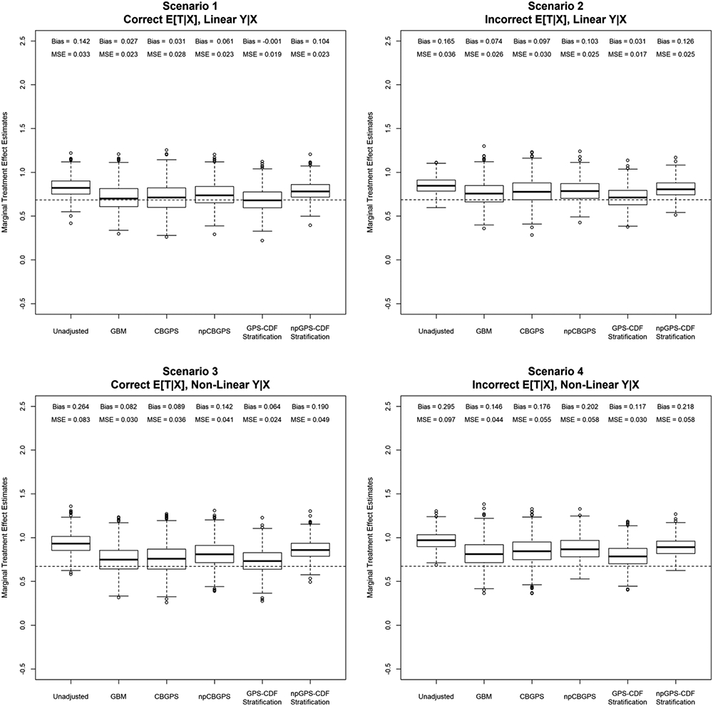
Distribution of the marginal treatment effect estimates for each method under each data generating scenario. Propensity models include only the true pretreatment confounders (x1, x2, x4, x5). The true marginal treatment effects are included as dotted horizontal lines in each plot.
In Scenario 1 (Figure 2), GPS-CDF stratification outperforms all other methods in terms of reduced bias and MSE. GPS-CDF stratification produces marginal treatment effect estimates with bias practically equal to zero. Alternatively, the bias and MSE achieved by npGPS-CDF stratification are worse than all other compared methods. When the treatment model is misspecified, but the outcome model is correct (Figure 2, Scenario 2), results are similar to Scenario 1. GPS-CDF stratification again produces the lowest bias and MSE compared to the other propensity score methods. Additionally, npCBGPS produces higher bias compared to the other weighting methods.
When the treatment model is correct, but the outcome model is misspecified (Figure 2, Scenario 3), application of GBM results in lower bias and MSE compared to CBGPS. Consistent with the previous scenarios, CBGPS outperforms npCBGPS, but both methods produce biased marginal treatment effect estimates. GPS-CDF stratification has lower bias and MSE compared to all other methods. Again npGPS-CDF stratification produces more biased estimates than all other compared methods. Finally, in Scenario 4 (Figure 2), weighting procedures, GBM, CBGPS, and npCBGPS, do not perform as well as GPS-CDF stratification. While none of the methods produce marginal treatment effect estimates with zero bias, the novel GPS-CDF method greatly outperforms all other propensity score methods with lower bias and MSE.
Further simulations are conducted that included all nine baseline covariates within the propensity score models (Supplemental Figure 1). Within this setting, GPS-CDF stratification again produces better covariate balance than all other propensity score methods. Additionally, the balance achieved by npGPS-CDF stratification is less sensitive to model misspecification compared to the three weighting methods, which produce F-statistic outliers. In terms of marginal treatment effects estimates, GPS-CDF stratification produces smaller bias and MSE, within Scenario 1, than all weighting methods, but no propensity score methods achieve unbiased results within Scenario 4.
Finally, additional simulations are conducted using previously published simulation scenarios (Appendix).24 These additional simulations do demonstrate situations where weighting based approaches may outperform GPS-CDF stratification in terms of achieved covariate balance. Within both investigated scenarios, GBM, CBGPS, npCBGPS, and GPS-CDF stratification produce minimally biased treatment effect estimates with low MSE.
4. Data Application: Effect of exposure to smoking imagery on smoking initiation in Mexican-American youth
To assess the utility of the novel continuous propensity scoring techniques, GPS-CDF stratification and npGPS-CDF stratification are applied to the Mexican-American Tobacco use in Children (MATCh) study to determine whether exposure to smoking imagery in movies influences smoking initiation among Mexican-American adolescents.43
The MATCh study was a longitudinal population-based cohort study among Mexican-American teens in Houston, Texas, that aimed to measure factors that influence an adolescent’s decision to experiment with cigarettes.44 One of the predictors of interest, exposure to smoking imagery in movies (SIM), was measured using a previously validated method in which subjects indicate whether or not they had viewed 50 randomly selected movies from a pool of 250. A scaled continuous variable which quantifies a subject’s exposure to SIM was then calculated.45
Typically, the continuous SIM exposure variable is categorized into four ordinal exposure groups. A previous ordinal propensity score analysis of these data determined that the odds of smoking initiation among teens significantly increased as their level of exposure to smoking imagery quartile increased (stratified ordinal propensity score OR=1.53, 95% CI [1.15, 2.03], p= 0.004).17 Although this method of categorization is not inappropriate, categorization of a continuous treatment variable may lead to loss of information during the outcome analysis.18,24 The GPS-CDF stratification and npGPS-CDF stratification methods allow one to treat SIM exposure as a continuous covariate to assess its relationship with smoking initiation in adolescents.
Several potential pre-exposure confounders (that are associated with both the level of exposure to smoking imagery in movies and smoking initiation) are included in the current analyses (Supplemental Table 1). Details of all variables included in the propensity models can be found in previous publications.17,46 A visual representation of covariate balance is shown in Figure 3. The figure presents F-statistics that are calculated by regressing the continuous treatment variable against each potential confounder one at a time. The interquartile range of F-statistics within the figure are (2.52-20.08) for the original data, (0.39-0.92) for GPS-CDF stratification, and (0.75-2.21) for npGPS-CDF stratification. As both propensity score stratification methods produce small F-statistics, they result in much better balance compared to the original data.
Figure 3.

Graphical representation of the covariate balance achieved by GPS-CDF and npGPS-CDF stratification within the MATCh study. The plot presents F-statistics obtained from regressing T on each potential confounder one at a time.
Outcome analyses of the MATCh study are re-conducted using GPS-CDF and npGPS-CDF stratification. Conditional logistic regression is used to estimate the marginal treatment effect for both stratification methods. Bootstrapping, which accounts for the variation in estimating the GPS, is used in order to estimate the standard error of the treatment effect estimates.18,38,39 Briefly, 1,000 bootstrap replicates are derived with replacement from the original study dataset. Within each of the bootstrap samples, the marginal treatment effect is estimated using both proposed stratification methods. The standard deviation of these estimates, across the bootstrap samples, is used as the estimate of the marginal treatment effect standard error.18,38 The derived standard errors are nearly equivalent to conditional regression standard errors found using the original data for both proposed methods.
The novel methods show that the odds of smoking initiation among teenagers significantly increases as exposure to SIM increases (ORGPS-CDF = 3.03, 95% CI [1.27, 7.20], p = 0.0122; ORnpGPS-CDF = 4.71, 95% CI [2.06, 10.77], p = 0.0002). Both proposed stratification methods attenuate this relationship compared to the original unadjusted data (OR= 6.57, 95% CI [3.06, 14.14], p<0.0001), and show similar strength of association compared to the original analyses conducted using ordinal propensity score stratification (OR= 3.58, for exposure category 4 vs. 1).17 Although the effect estimates derived using the new methods are similar in magnitude to those previously reported, the association between exposure to SIM and smoking initiation can now be interpreted on the original exposure scale. Thus, an increase in exposure to smoking imagery by 10% would increase the odds of smoking initiation in adolescents 1.12 times.
For comparison, the three weighting methods examined in the above simulation study are also applied to the MATCh data analysis. These methods derived larger treatment effects than GPS-CDF stratification (ORGBM = 4.16, 95% CI [1.78, 9.66], p= 0.0010; ORCBGPS = 3.55, 95% CI [1.50, 8.35], p= 0.0038; ORnpCBGPS = 3.55, 95% CI [1.54, 8.14], p= 0.0028), which further demonstrates the utility of the GPS-CDF method to remove covariate imbalance from analyses. When running analyses using a dual-core Intel Core i3-3110M with 4 GB RAM, results were available in 7-8 seconds for the two new methods. Results were available in 28 seconds using GBM, 5 seconds for CBGPS, and 16 seconds for npCBGPS.
5. Discussion
Although weighting methods have been proposed to conduct propensity score analyses with continuous treatments,18,20,24 these methods are not always stable and may produce unreliable estimates. Through simulation, Fong et al. showed that MLE20 and GBM24 weights may result in worse covariate balance than had no adjustment been made.18 These authors further demonstrated that their newly developed weighting methods, CBGPS and npCBGPS, were able to produce better balance than both the MLE and GBM methods. Although the CBGPS methods aim to optimize covariate balance, this increased balance does not always provide more accurate estimates within the outcome analyses. When both treatment and outcome models were misspecified, they found that all weighting propensity score methods failed to obtain unbiased treatment effect estimates. Based on the inability of weighting procedures to produce both stable and accurate treatment effect estimates, we developed new continuous treatment propensity score stratification techniques, GPS-CDF and npGPS-CDF, and investigated their performance against other continuous treatment propensity score methods.
Our simulation study is stronger than some previously conducted,18,21 as it was representative of biomedical data through inclusion of both continuous and binary covariates. The inability of GBM weighting to produce reliable and accurate covariate balance was re-established within our simulation. When treatment assignment was both correctly and incorrectly specified, GBM weighting produced poor balance with patterns similar to a previous simulation.18 Unlike Fong et al., the CBGPS method did not optimize balance for all datasets within our simulations.18 Since CBGPS methods seek to minimize the weighted correlation between baseline covariates and the treatment, inclusion of binary covariates (as with our simulation) in the propensity score model may cause the CBGPS methods to fail, in terms of producing reliable covariate balance. Of note, we were able to fully replicate the results of Fong et al. using a simulation consisting of only continuous covariates (not presented),18 which in our opinion, is not generally applicable to biomedical research questions. Future studies should further evaluate the CBGPS method under additional simulation scenarios with differing covariate types in relation to achieved covariate balance.
Failure to achieve covariate balance when presented with both continuous and binary pretreatment confounders did not arise with the GPS-CDF stratification method. This novel method produced better balance than GBM, CBGPS, and npCBGPS within our simulation. Interestingly, GPS-CDF stratification produced better covariate balance than npGPS-CDF stratification. Within the binary treatment setting, Rubin showed that matching on a regression based scalar value produces better covariate balance than methods that match directly on covariates.47 As GPS-CDF stratification is implemented using a regression model and npGPS-CDF stratification balances directly on potential confounders, our findings in the continuous treatment setting are analogous and unsurprusing.47 These finding were further demonstrated via comparisons of the marginal treatment effect estimates.
Across all scenarios, GPS-CDF stratification outperformed npGPS-CDF stratification in terms of bias and MSE. Additionally, even though the balance achieved by npCBGPS weighting was comparable to CBGPS, for the incorrectly specified treatment model, npCBGPS produced treatment effect estimates with higher bias than CBGPS across all scenarios. This finding may further demonstrate that better covariate balance does not always lead to less biased causal inference estimates.48,49 Within Scenario 4, which contained misspecification in both the treatment and outcome models, GBM, CBGPS, and npCBGPS failed to obtain satisfactory marginal treatment effect estimates, which is consistent to the results presented by Fong et al.18 Importantly, our newly developed GPS-CDF stratification method was still robust, even when applied to models with misspecification. Finally, comparisons between simulations that only include pretreatment confounders in the propensity models (Figure 2) and those that include all baseline covariates (Supplemental Figure 1) demonstrate the importance of variable selection in propensity score analyses.40 Careful consideration should be applied when selecting variables to include in propensity models, as incorrect inclusion may lead to more biased treatment effect estimates.4,40
The utility and performance of the GPS-CDF methods was further demonstrated on the MATCh study. Our newly derived methods had low computational burden and produced better covariate balance than the original dataset. Furthermore, our stratification methods showed a similar association between the odds of smoking initiation and exposure to smoking imagery in movies in Mexican-American adolescents as previous ordinal propensity score analyses but allowed for interpretations based on the original scale of the continuous exposure.17 Based on these causal findings, future studies should further evaluate smoking imagery as a possible modifiable exposure for at-risk youth.
There are limitations with the current study. Primarily, there is no theoretical support that the proposed stratification methods offer the same balancing properties as the original GPS.1 However, there is extensive empirical evidence, offered through simulation scenarios representative of real-world data,17,18,41 that shows GPS-CDF stratification out performs standard weighting-based approaches. Additionally, both proposed stratification methods were computed using 5 strata.11,35-37 The choice of number of strata may greatly affect both covariate balance and the amount of bias removed within analyses. As the proposed methods utilize stratification, there is the possibility of not fully accounting for bias, as has been shown with binary treatments.50 Furthermore, truncation was applied to all weighting based procedures to remove the possible effects of large weights.21 While any level of percentile truncation may be applied to weighting procedures, progressive truncation of weights should be applied with caution, as this can lead to manipulated findings equal to a desired result.3,51 Therefore, as with all propensity score analyses, investigators should select and implement the propensity score method that achieves the best covariate balance for their specific data.
In summary, this paper details the derivation and application of two stratification propensity scoring methods that remove imbalance due to confounding in observational studies with continuous treatments. Unlike current methods of continuous treatment propensity scoring that utilize weighting, the GPS-CDF and npGPS-CDF methods presented here, create balancing strata that contain subjects with similar covariate distributions. These novel methods allow investigators additional options when conducting continuous treatment propensity scoring in both parametric (GPS-CDF) and nonparametric (npGPS-CDF) frameworks. As with all propensity score methods, investigators should select the method that creates the best covariate balance for their data. Future research should further investigate the use of stratification techniques when conducting continuous treatment propensity scoring with applications to relevant public health research questions.
Supplementary Material
Acknowledgment
This work was supported by the National Institute of General Medical Sciences training grant T32 GM074902 and by the Intramural Research Program of the US National Cancer Institute. The opinions expressed by the authors are their own and this material should not be interpreted as representing the official viewpoint of the U.S. Department of Health and Human Services, the National Institutes of Health or the National Cancer Institute.
Data Availability
The data that support the findings of this study are available on request from the corresponding author. The data are not publicly available due to privacy or ethical restrictions.
References
- 1.Hirano K, Imbens GW. The propensity score with continuous treatments. Applied Bayesian modeling and causal inference from incomplete-data perspectives. 2004;226164:73–84. [Google Scholar]
- 2.Austin PC, Stuart EA. Moving towards best practice when using inverse probability of treatment weighting (IPTW) using the propensity score to estimate causal treatment effects in observational studies. Statistics in medicine. 2015;34(28):3661–3679. [DOI] [PMC free article] [PubMed] [Google Scholar]
- 3.Cole SR, Hernán MA. Constructing inverse probability weights for marginal structural models. Am J Epidemiol. 2008;168(6):656–664. [DOI] [PMC free article] [PubMed] [Google Scholar]
- 4.Austin PC. The performance of different propensity score methods for estimating marginal odds ratios. 2007;26(16):3078–3094. [DOI] [PubMed] [Google Scholar]
- 5.Stampf S, Graf E, Schmoor C, Schumacher MJSim. Estimators and confidence intervals for the marginal odds ratio using logistic regression and propensity score stratification. 2010;29(7-8):760–769. [DOI] [PubMed] [Google Scholar]
- 6.Stürmer T, Joshi M, Glynn RJ, Avorn J, Rothman KJ, Schneeweiss SJJoce. A review of the application of propensity score methods yielded increasing use, advantages in specific settings, but not substantially different estimates compared with conventional multivariable methods. 2006;59(5):437. e431–437. e424. [DOI] [PMC free article] [PubMed] [Google Scholar]
- 7.Imai K, Van Dyk DA. Causal inference with general treatment regimes: Generalizing the propensity score. Journal of the American Statistical Association. 2004;99(467):854–866. [Google Scholar]
- 8.Imbens GW. The role of the propensity score in estimating dose-response functions. Biometrika. 2000;87(3):706–710. [Google Scholar]
- 9.Joffe MM, Rosenbaum PR. Invited commentary: propensity scores. American journal of epidemiology. 1999;150(4):327–333. [DOI] [PubMed] [Google Scholar]
- 10.Rosenbaum PR, Rubin DB. The Central Role of the Propensity Score in Observational Studies for Causal Effects. Biometrika. 1983;70(1):41–55. [Google Scholar]
- 11.Rosenbaum PR, Rubin DB. Reducing bias in observational studies using subclassification on the propensity score. Journal of the American statistical Association. 1984;79(387):516–524. [Google Scholar]
- 12.Rosenbaum PR, Rubin DB. Constructing a control group using multivariate matched sampling methods that incorporate the propensity score. The American Statistician. 1985;39(1):33–38. [Google Scholar]
- 13.Brown DW, DeSantis SM, Greene TJ, et al. A novel approach for propensity score matching and stratification for multiple treatments: Application to an electronic health record-derived study. Statistics in medicine. 2020;39(17):2308–2323. [DOI] [PMC free article] [PubMed] [Google Scholar]
- 14.Boyd CL, Epstein L, Martin AD. Untangling the causal effects of sex on judging. American journal of political science. 2010;54(2):389–411. [Google Scholar]
- 15.Chertow GM, Normand S-LT, McNeil BJ. “Renalism”: inappropriately low rates of coronary angiography in elderly individuals with renal insufficiency. Journal of the American Society of Nephrology. 2004;15(9):2462–2468. [DOI] [PubMed] [Google Scholar]
- 16.Davidson MB, Hix JK, Vidt DG, Brotman DJ. Association of impaired diurnal blood pressure variation with a subsequent decline in glomerular filtration rate. Archives of internal medicine. 2006;166(8):846–852. [DOI] [PubMed] [Google Scholar]
- 17.Greene TJ. A Novel Non-Parametric Method for Ordinal Propensity Score Stratification and Matching. 2017. [DOI] [PMC free article] [PubMed] [Google Scholar]
- 18.Fong C, Hazlett C, Imai K. Covariate balancing propensity score for a continuous treatment: Application to the efficacy of political advertisements. The Annals of Applied Statistics. 2018;12(1):156–177. [Google Scholar]
- 19.Royston P, Altman DG, Sauerbrei W. Dichotomizing continuous predictors in multiple regression: a bad idea. Statistics in medicine. 2006;25(1):127–141. [DOI] [PubMed] [Google Scholar]
- 20.Robins JM, Hernan MA, Brumback B. Marginal structural models and causal inference in epidemiology. In: LWW; 2000. [DOI] [PubMed] [Google Scholar]
- 21.Austin PC. Assessing the performance of the generalized propensity score for estimating the effect of quantitative or continuous exposures on binary outcomes. Statistics in medicine. 2018;37(11):1874–1894. [DOI] [PMC free article] [PubMed] [Google Scholar]
- 22.Austin PC. Assessing covariate balance when using the generalized propensity score with quantitative or continuous exposures. Statistical methods in medical research. 2018:0962280218756159. [DOI] [PMC free article] [PubMed] [Google Scholar]
- 23.Schuler MS, Chu W, Coffman D. Propensity score weighting for a continuous exposure with multilevel data. Health Services and Outcomes Research Methodology. 2016;16(4):271–292. [DOI] [PMC free article] [PubMed] [Google Scholar]
- 24.Zhu Y, Coffman DL, Ghosh D. A boosting algorithm for estimating generalized propensity scores with continuous treatments. Journal of causal inference. 2015;3(1):25–40. [DOI] [PMC free article] [PubMed] [Google Scholar]
- 25.Kreif N, Grieve R, Diaz I, Harrison D. Evaluation of the Effect of a Continuous Treatment: A Machine Learning Approach with an Application to Treatment for Traumatic Brain Injury. Health economics. 2015;24(9):1213–1228. [DOI] [PMC free article] [PubMed] [Google Scholar]
- 26.Wu X, Mealli F, Kioumourtzoglou M-A, Dominici F, Braun D. Matching on generalized propensity scores with continuous exposures. arXiv preprint arXiv:181206575. 2018. [DOI] [PMC free article] [PubMed] [Google Scholar]
- 27.Kang JD, Schafer JL. Demystifying double robustness: A comparison of alternative strategies for estimating a population mean from incomplete data. Statistical science. 2007;22(4):523–539. [DOI] [PMC free article] [PubMed] [Google Scholar]
- 28.Bia M, Flores CA, Flores-Lagunes A, Mattei A. A Stata package for the application of semiparametric estimators of dose–response functions. Stata Journal. 2014;14(3):580–604. [Google Scholar]
- 29.McCaffrey DF, Griffin BA, Almirall D, Slaughter ME, Ramchand R, Burgette LF. A tutorial on propensity score estimation for multiple treatments using generalized boosted models. Statistics in medicine. 2013;32(19):3388–3414. [DOI] [PMC free article] [PubMed] [Google Scholar]
- 30.Ridgeway G, McCaffrey D, Morral A, Griffin B, Burgette L. Toolkit for Weighting and Analysis of Nonequivalent Groups (Version 1.4-9.5). In:2016. [Google Scholar]
- 31.Imai K, Ratkovic M. Covariate balancing propensity score. Journal of the Royal Statistical Society: Series B (Statistical Methodology). 2014;76(1):243–263. [Google Scholar]
- 32.Marquardt DW. An algorithm for least-squares estimation of nonlinear parameters. Journal of the society for Industrial and Applied Mathematics. 1963;11(2):431–441. [Google Scholar]
- 33.Bates DM, Watts DG. Nonlinear regression analysis and its applications. Vol 2: Wiley; New York; 1988. [Google Scholar]
- 34.Tu C, Jiao S, Koh WY. Comparison of clustering algorithms on generalized propensity score in observational studies: a simulation study. Journal of Statistical Computation and Simulation. 2013;83(12):2206–2218. [Google Scholar]
- 35.Austin PC. An Introduction to Propensity Score Methods for Reducing the Effects of Confounding in Observational Studies. Multivariate Behavioral Research. 2011;46(3):399–424. [DOI] [PMC free article] [PubMed] [Google Scholar]
- 36.Cochran WG. The effectiveness of adjustment by subclassification in removing bias in observational studies. Biometrics. 1968:295–313. [PubMed] [Google Scholar]
- 37.Zanutto E, Lu B, Hornik R. Using propensity score subclassification for multiple treatment doses to evaluate a national antidrug media campaign. Journal of Educational and Behavioral Statistics. 2005;30(1):59–73. [Google Scholar]
- 38.Austin PC, Small DS. The use of bootstrapping when using propensity-score matching without replacement: a simulation study. Statistics in medicine. 2014;33(24):4306–4319. [DOI] [PMC free article] [PubMed] [Google Scholar]
- 39.Lopez MJ, Gutman R. Estimation of causal effects with multiple treatments: a review and new ideas. Statistical Science. 2017;32(3):432–454. [Google Scholar]
- 40.Brookhart MA, Schneeweiss S, Rothman KJ, Glynn RJ, Avorn J, Stürmer T. Variable selection for propensity score models. American journal of epidemiology. 2006;163(12):1149–1156. [DOI] [PMC free article] [PubMed] [Google Scholar]
- 41.Austin PC, Grootendorst P, Anderson GM. A comparison of the ability of different propensity score models to balance measured variables between treated and untreated subjects: a Monte Carlo study. Statistics in medicine. 2007;26(4):734–753. [DOI] [PubMed] [Google Scholar]
- 42.Huang I-C, Frangakis C, Dominici F, Diette GB, Wu AW. Application of a propensity score approach for risk adjustment in profiling multiple physician groups on asthma care. Health services research. 2005;40(1):253–278. [DOI] [PMC free article] [PubMed] [Google Scholar]
- 43.Wilkinson AV, Waters AJ, Vasudevan V, Bondy ML, Prokhorov AV, Spitz MR. Correlates of susceptibility to smoking among Mexican origin youth residing in Houston, Texas: a cross-sectional analysis. BMC Public Health. 2008;8(1):337. [DOI] [PMC free article] [PubMed] [Google Scholar]
- 44.Spelman AR, Spitz MR, Kelder SH, et al. Cognitive susceptibility to smoking: Two paths to experimenting among Mexican origin youth. Cancer epidemiology, biomarkers & prevention : a publication of the American Association for Cancer Research, cosponsored by the American Society of Preventive Oncology. 2009;18(12):3459–3467. [DOI] [PMC free article] [PubMed] [Google Scholar]
- 45.Sargent JD, Worth KA, Beach M, Gerrard M, Heatherton TF. Population-based assessment of exposure to risk behaviors in motion pictures. Communication Methods and Measures. 2008;2(1-2):134–151. [DOI] [PMC free article] [PubMed] [Google Scholar]
- 46.Wilkinson AV, Spitz MR, Prokhorov AV, Bondy ML, Shete S, Sargent JD. Exposure to smoking imagery in the movies and experimenting with cigarettes among Mexican heritage youth. Cancer epidemiology, biomarkers & prevention : a publication of the American Association for Cancer Research, cosponsored by the American Society of Preventive Oncology. 2009;18(12):3435–3443. [DOI] [PMC free article] [PubMed] [Google Scholar]
- 47.Rubin DB. Matched Sampling for Causal Effects. Cambridge University Press; 2006. [Google Scholar]
- 48.Lee BK, Lessler J, Stuart EA. Improving propensity score weighting using machine learning. Statistics in medicine. 2010;29(3):337–346. [DOI] [PMC free article] [PubMed] [Google Scholar]
- 49.Stuart EA, DuGoff E, Abrams M, Salkever D, Steinwachs D. Estimating causal effects in observational studies using Electronic Health Data: Challenges and (some) solutions. EGEMS (Washington, DC). 2013;1(3). [DOI] [PMC free article] [PubMed] [Google Scholar]
- 50.Schafer JL, Kang J. Average causal effects from nonrandomized studies: a practical guide and simulated example. Psychol Methods. 2008;13(4):279–313. [DOI] [PubMed] [Google Scholar]
- 51.Lee BK, Lessler J, Stuart EAJPo. Weight trimming and propensity score weighting. 2011;6(3):e18174. [DOI] [PMC free article] [PubMed] [Google Scholar]
Associated Data
This section collects any data citations, data availability statements, or supplementary materials included in this article.
Supplementary Materials
Data Availability Statement
The data that support the findings of this study are available on request from the corresponding author. The data are not publicly available due to privacy or ethical restrictions.