

Abstract
Linear response theory relates the response of a system to a weak external force with its dynamics in equilibrium, subjected to fluctuations. Here, this framework is applied to financial markets; in particular we study the dynamics of a set of stocks from the NASDAQ during the last 20 years. Because unambiguous identification of external forces is not possible, critical events are identified in the series of stock prices as sudden changes, and the stock dynamics following an event is taken as the response to the external force. Linear response theory is applied with the log-return as the conjugate variable of the force, providing predictions for the average response of the price and return, which agree with observations, but fails to describe the volatility because this is expected to be beyond linear response. The identification of the conjugate variable allows us to define the perturbation energy for a system of stocks, and observe its relaxation after an event.
Subject terms: Statistical physics, Nonlinear phenomena
Introduction
Linear response theory (LRT)1, allows resolving the response of a system to a weak external perturbation considering the dynamics of the system at equilibrium subjected to fluctuations. This is a practical extension of Onsager’s regression hypothesis, namely, a system relaxes to equilibrium after an external perturbation in a similar manner as from fluctuations2. This powerful tool and the formalism of time correlation functions have been applied to study several physical systems, such as soft matter3–6, spin glasses7, or magnetism8, but also it has been used to derive a conceptual basis for equilibrium and non-equilibrium thermodynamics9,10. The drawback is that only the first order in the perturbation is retained, which might not be sufficient in some cases11.
In LRT, a linear perturbation to the equilibrium Hamiltonian of the system is assumed, , where denotes the Hamiltonian in the equilibrium (non-perturbed) state, and the perturbation, with F the external force, which is conjugate to the variable A. The theory restricts to small forces, and states that the change in a variable B(t) due to the application of the force is given by1,12:
| 1 |
where the after-effect function is set by the correlation function:
| 2 |
which is calculated in the unperturbed (equilibrium) state, with the inverse thermal energy, and denotes the time derivative of A. LRT, both in the classical and quantum forms, have been applied mainly to the calculation of transport coefficients in several systems, such as colloids, charge transport, ferromagnetization or liquid crystals13, but also in other more exotic fields, such as neurophysiology14 or climate science15,16. In this paper, we aim to apply LRT to a very different field, namely, stock markets.
The application of physical theories and models to financial markets has attracted interest since the work of Bachelier in 190017, and in particular in the last three decades18–21. Most models or applications describe financial market dynamics as equilibrium systems subjected to fluctuations, fulfilling the fluctuation–dissipation theorem22, such as a Brownian particle or system23–26, while other works try to analyze its entropy or complexity27,28. The non-Gaussianity of fluctuations causing anomalous diffusion has also received attention from the early works of Mandelbrot29,30, where elaborate models to describe such fluctuation distributions have been resolved, e.g., by considering truncated Levy flights31,32, the Tsallis entropy model33,34, hopping in the free energy landscape in glasses35–37, or extending the continuous-time random walk model38,39.
Within a Physics scope, regime switching models have been applied to market dynamics40. Such transition is straightforward for instance in changes in economic policy, such as the Quantitative Easing policies from the European Central Bank (ECB) and the Federal Reserve Board (FED)41,42, or abrupt when unexpected events occur, such is the case of the Great Recession from 2008, or the still ongoing crisis due to the spread of the COVID-19 pandemics43–45. Such regimes are characterized according to economic and business cycles of expansion and recession46. There, different classes of random walks have been identified, where the nature of price changes are resolved not due to the unpredictable nature of incoming news but a direct consequence of competition between market forces led by liquidity and market takers and makers47. Long-range correlated market orders and activity lead to diffusive and super-diffusive dynamics, while mean reverting limit orders determine sub-diffusive market conditions36,47. In such framework, the linear response formalism has been considered when studying casual relations in markets, where characteristic volatility and stock dynamic regimes are identified as influencing the overall market dynamics prior to financial crashes, while individual volatility of securities follow collective market behavior after the crash event48. Moreover, the breakdown of linear response has been found in periods of low market liquidity and transaction, where fluctuations become large enough so that market dynamics is strongly displaced from equilibrium, and second or larger order energy terms must be accounted for in the Hamiltonian of the system49.
Our aim in this work is to apply LRT to a system of stocks, thus enlarging the applicability of LRT and also advancing in the knowledge of the mechanisms governing the stock dynamics. For this purpose, a given financial market is assumed to be an equilibrium system subjected to fluctuations due to its internal dynamics, and perturbed by external forces. Within LRT we attempt to study weak forces, where the effects are linear with force strength. LRT can provide then the evolution of the system after the application of the external force. Thus, for this analysis the following steps have been followed: (1) measurement of the response of the system after the application of an external perturbation, (2) identification of the variable A(t), conjugate to the force, and (3) calculation of the response function according to LRT, to finally compare it with the “empirical” function obtained in (1). As a final result, in addition to the extension of LRT, the perturbation energy in a stock market can be defined. Note that since we do not base the identification of the variable conjugate on a physical model, we only rely only on the validity of LRT for stock markets.
A database of 862 stocks has been used, corresponding to the companies in the NASDAQ index from 03/01/2000 to 30/10/2020. The “Supplementary Information” to this article provides a similar analysis for a set of European stocks and the NYSE, yielding similar results.
Results
Consider a charged colloidal particle in water: internal forces are caused by thermal and density fluctuations in the solvent and provoke the particle Brownian motion, whereas external forces can be caused by electric or gravitational fields50. Stock prices, on the other hand, are set by brokers or other practitioners, according to supply and demand, as well as to their investment strategies and expectations; these can be considered as internal forces. However, there are factors that strongly influence market prices, such as political decisions, announcements of results, companies acquisition or merger, bankrupts, ... These can be considered as external forces, which, different from the physical counterpart, act onto the stock prices through the same practitioners as the internal forces. This ambiguous recognition of external forces poses a major problem on their identification, as well as its strength scale, and the conjugate variable A(t), needed for the application of the LRT formalism. In fact, it is generally accepted that only a fraction of the motion of stocks can be attributed to fundamental economic information that could have had a pronounced impact on cash flow forecasts or discount rates51,52.
Therefore, we do not make any assumptions concerning external forces, and adopt a phenomenological point of view following previous works on events53: a dramatic event, assumed to be provoked by an external force, takes place whenever the absolute value of the one day log-return of a stock surpasses four times the root mean square deviation of log-returns of this stock. This threshold for the definition of an event is arbitrary but in line with previous studies54, as it allows the segmentation of events in equilibrium fluctuations or dramatic perturbations. In any case, its specific value has little effect on the results presented below, as far as it is well above 1. In the following, we assume that the external force starts to act at the event time , and keeps acting indefinitely, or until a new event takes place. Furthermore, we assume that the impact of different forces are well separated, i.e. the evolution of a stock price after a force is applied relaxes to equilibrium before a new force acts; thus events separated less than 10 days are discarded. With such criteria, ca. 5000 events are identified in the whole set ( positive events, with positive log-return , and negative ones, with ). Note that very dramatic events, such as the financial crisis in 2008 or the COVID19 pandemic in 2020, provoke drastic changes in the price extending over several days54,55, and are excluded from our analysis according to this selection, because LRT is expected to fail for large external forces. The resulting distribution of events per day (affecting different stocks) is a decreasing function, with 75% of the events in days with less than five events, which guarantees that the events are indeed independent. Fig. 1 analyzes the stock log-price after an event, namely the response function of the log-price after an event”.
Figure 1.

Analysis of events. Left panel (A) distribution of the relative total log-price variation (circles), with a Gaussian fitting to the maximum (red line). Right panel (B) evolution of the log-price before and after small events in absolute value (circles). The inset shows positive and negative events separatedly. The lines are the prediction from LRT (see text below).
Figure 1A presents the distribution of the total log-price variations provoked by the event, namely , where is the log-price just before the event, and is the log-price well after the event. The local minimum at is caused by our definition of events, and disappears if a smaller threshold is selected. On the other hand, the distribution displays positive deviations from Gaussian behaviour for price differences above in absolute value. These deviations are typical in finance, and have been the topic of intense research and debate21. To our purpose, the deviation from the Gaussian profile serves to identify “small” and “large” events, and therefore determine the expected validity range of LRT. All subsequent analysis is restricted to small events. In Fig. 1B the mean normalized log-price evolution around the event in absolute value is presented. This shows an overshoot at , namely when the event takes place, followed by a decay within a few days to reach a steady value ( is the average log-price between 10 and 20 days after the event). The inset shows positive and negative events separatedly.
In addition to the log-price, the dynamics of stocks is also monitored considering the corresponding log-return and volatility. (The latter represents how fast the price changes, irrespective of the sign of the change, and is calculated as ). The average normalized evolution of the one day return and volatility after an event are shown in Fig. 2. The average log-return for a positive (negative) event increases (decreases) at the event, and decreases (increases) abruptly immediately after it, followed by a slow relaxation to the equilibrium value. The figure represents the normalized evolution averaged for positive and negative events. The volatility, on the other hand, increases at and then decreases to the “equilibrium” magnitude at both positive and negative events.
Figure 2.
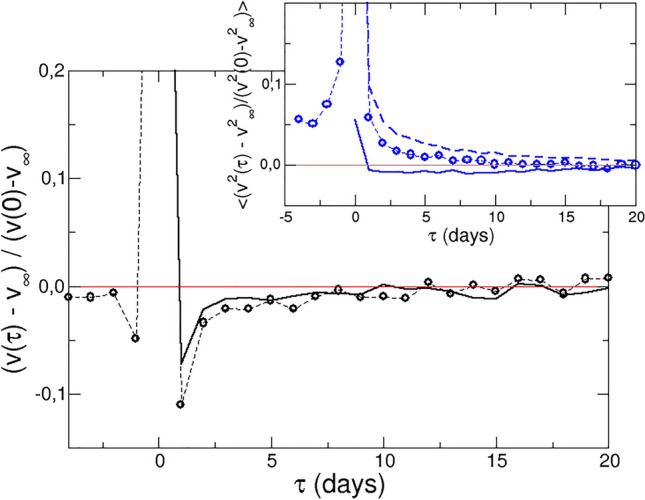
Evolution of the log-return and the volatility (inset) before and after small positive and negative events. The lines show the prediction of linear response theory (see text below).
Figures 1 and 2 show that the evolution of the log-price, log-return and volatility is abrupt at the event, and then relaxes to a steady value for a few days. From a physical point of view, this indicates that these variables display memory, and according to LRT, the correlation functions with variable A(t), conjugate of the force, should decay with a time scale of a few days. In order to identify this variable, the log-price, log-return and volatility autocorrelation functions (ACF) have been studied (see “Methods”).
They are presented in Fig. 3 and show very different behaviour: whereas the log-return reaches negative values within the first day and then relaxes to zero (resembling the velocity ACF in hard spheres), and the volatility ACF presents a similar time scale, but a monotonous decay, the time scale of the log-price ACF is days. For the purpose of applying LRT, the log-return is more appropriate due to the similarity with the time scale and behaviour of its response function. Therefore, we tentatively identify the log-return, v(t), as the conjugate variable, A(t), to the external force. The response of the log-return is therefore provided directly by its ACF, assuming that the force follows a Heaviside functional form, as discussed above:
| 3 |
Figure 3.

Autocorrelation functions of the log-price (red line and circles), log-return (continuous black line) and volatility (broken blue line).
Since the strength of the force is unknown, we plot to compare with the normalized response of the log-return in Fig. 2 (black line). The prediction from LRT agrees with the empirical response function.
Once the conjugate variable, A(t) in Eq. (1), has been identified as the log-return, the average evolution of other variables can be readily obtained using LRT. In particular, for the log-price, the integral of the log-return ACF above provides the predicted response, according to LRT:
| 4 |
since . This is included also in the right panel of Fig. 1. Again, good agreement between this prediction and the observations is found. Similar comparisons between the predictions from LRT and the evolution of the log-price and log-return for a set of European stocks and for the NYSE are presented in Figs. 1 and 3 of the “Supplementary Information”. Note that in any case, LRT predicts the average response of the variable, and cannot be used to calculate the evolution of a single stock (or in physical terms, of a single trajectory in phase space).
The volatility, on the other hand, is a second-order variable and it is not expected that it can be described within LRT. This is tested in the inset to Fig. 2, where the cross correlation function is included (continuous line), as well as the volatility ACF (broken line). None of them correctly describes the observed evolution of the volatility, although the predction from LRT (continuous line), captures qualitatively the slow decay of the volatility after the event.
For constant external forces, LRT also provides the coupling constant of the system in the stationary regime as the integral of extended to , i.e., . For the case of autocorrelation functions, these constants are the transport coefficients associated with the flux induced by the external force, and depict the Green–Kubo relations56. In our case, two coefficients can be calculated:
| 5 |
Note that the correlation function is used here, instead of the normalized C(v, v) used above.
To test these results, we display in Fig. 4 the average total variation of the log-return, as a function of the log-price total variation, for small events. The expected linear relationships with the force, yield , which is also included in Fig. 4. The data show good agreement with the predictions, particularly for small price variations, where the theory is expected to perform better. For the volatility, the total variation has been also included in the figure as a function of the log-price variation, but the dependence is clearly not linear.
Figure 4.

Mean log-return and volatility variations as a function of the total log-price variation for small events, as labelled. The solid red line indicates the prediction for the log-return.
Table 1 presents the results of the coefficients and for the NYSE and European sets of stocks, studied in more detail in the “Supplementary Information”. The concomitant tests of the linearity of vs. are also presented there. Note that and are much larger (in absolute value) for the NASDAQ and NYSE than for the European stocks, implying that the European set is less affected by external forces, probably due to its heterogeneity.
Table 1.
Values of the coefficients and for the three sets of stocks considered.
| Stock market | ||
|---|---|---|
| NASDAQ | ||
| NYSE | ||
| European |
Once variable A has been identified as the log-return, the perturbation energy can be calculated if the force is known. Nevertheless, within the linear regime, the total log-price variation is proportional to the force, , and the energy can be calculated as:
| 6 |
The distribution of perturbation energies shows a symmetric bell shape with the expected wings or tails for large (positive and negative) values. Since for both positive and negative events the product is positive at the event, the sign of determines if the energy is positive or negative for both types of events. Our calculations yield a negative , which corresponds to a negative perturbation energy, with respect to the value just before the event.
Figure 5 presents this energy for both kinds of events. The energy is near zero before and well after the event, when its effect has dissipated, but grows (in absolute value) notably for all events. This effect dissipates as equilibrium is recovered. From a physical perspective, this is equivalent to a system where the energy input dissipates and the system returns to equilibrium. The time scale for the dissipation is the same as for the decay of the log-return ACF, as the force is continuously active for . Interestingly, the figure indicates that the perturbation energy is also non-zero for , i.e., before the event. This is beyond our current interpretation of the results, where the force can only affect the system for positive times, but could be tackled with a time dependent force. Also, such feature could serve as an indicator of an event in the next few days. Nevertheless, it must be recalled that our modeling considers averages over many different events in 20 years and a set of ca. 850 stocks. Thus, predicting events to a single stock is far beyond the purpose of this work.
Figure 5.

Perturbation energy for positive (black circles) and negative events (red crosses).
Discussion
We have resolved Linear Response Theory as an efficient framework to determine the response of a system such as the stock market, which is indeed hallmarked by fluctuations. The autocorrelation functions of the log-price, log-return, and volatility indicate that the most appropriate variable to be considered conjugate of the external force is the log-return, due to its relaxation kinetics. Thus, the predicted response functions for the log-price and log-return have been calculated and agree with the results obtained from the empirical analysis of stock prices. Both of them show an overshoot at the event, and a slower recovery towards equilibrium within 2–3 days, in resemblance with the behaviour of a dissipative system. The identification of the energy in a stock market represents a major goal, strikingly supported on a well-established physical ground.
The results presented here have been obtained for the NASDAQ, extending over the last 20 years considering the stocks that have belonged continuously to the index. Similar results have been also obtained for a set of European national floors, although the statistics is much better in the case of the NASDAQ, and New York Stock Exchange. These results provide further support of the results and conclusions presented here.
In any case, we stress that there is no physical model supporting this identification of the log-return as conjugate to the external force. The results presented here are based on a phenomenological approach, but show the compatibility of financial markets with well-established physical theories, as far as an appropriate analogy of variables is performed.
Methods
All stocks used for this study have been taken from Yahoo! Finance, with a time resolution of 1 day. The databases have been comprised by all stocks that have belonged continuously to the given market. For the NASDAQ (main text) and NYSE (“Supplementary Information”), stocks that have been active from 03/01/2000 to 30/10/2020 were selected, amounting to 862 stocks and 1084, respectively. For the european stocks, the set of stocks is constructed with companies that have belonged continuously to the national indices of the UK (FTSE100), Germany (DAX30), France (CAC40), Spain (IBEX35), Switzerland (SMI), Italy (FTSE MIB), Portugal (PSI20), and Holland (AEX). This set comprises 240 stocks, corresponding to big and stable European companies, sampled every day since 2010–2019.
As usual in financial studies, we consider the logarithm of the price, termed log-price, and only working days in the analysis, i.e. weekends are not taken into account. The one-day log-return is defined as and the volatility is calculated as .
A dramatic event, assumed to be provoked by an external force, takes place whenever the absolute value of the one day log-return of a stock surpasses four times the root mean square deviation of log-returns of this stock, i.e., if:
| 7 |
where is the total number of days in our sample.
The time auto-correlation function between the discrete variables X and Y, and , with , is calculated as:
where and stand for the sample mean and standard deviation, respectively.
The non-normalized correlation function, , has also been used to calculate the coefficients and . This is defined as:
Supplementary Information
Acknowledgements
Authors gratefully acknowledge Prof. Dr. Matthias Fuchs for fruitful discussions and feedback. Financial support for this work was obtained from the Spanish Ministerio de Ciencia, Project No. PGC2018-101555-B-I00, and Universidad de Almería, Project No. UAL18-FQM-B038-A (UAL/CECEU/FEDER).
Author contributions
All authors contributed equally to the design of the methodology, discussion, analysis and revisions of the manuscript.
Competing interests
The authors declare no competing interests.
Footnotes
Publisher's note
Springer Nature remains neutral with regard to jurisdictional claims in published maps and institutional affiliations.
Supplementary Information
The online version contains supplementary material available at 10.1038/s41598-021-02263-6.
References
- 1.Kubo R. Statistical-mechanical theory of irreversible processes. I. General theory and simple applications to magnetic and conduction problems. J. Phys. Soc. Jpn. 1957;12:570–586. [Google Scholar]
- 2.Onsager L. Reciprocal relations in irreversible processes. I. Phys. Rev. 1931;37:405–426. [Google Scholar]
- 3.Benetatos P, Frey E. Linear response of a grafted semiflexible polymer to a uniform force field. Phys. Rev. E. 2004;70:051806. doi: 10.1103/PhysRevE.70.051806. [DOI] [PubMed] [Google Scholar]
- 4.Boschan J, Vasudevan SA, Boukany PE, Somfai E, Tighe BP. Stress relaxation in viscous soft spheres. Soft Matter. 2017;13:6870–6876. doi: 10.1039/c7sm01700f. [DOI] [PubMed] [Google Scholar]
- 5.Vogel F, Zippelius A, Fuchs M. Emergence of Goldstone excitations in stress correlations of glass-forming colloidal dispersions. Europhys. Lett. 2019;125:68003. [Google Scholar]
- 6.Dal Cengio S, Levis D, Pagonabarraga I. Linear response theory and Green–Kubo relations for active matter. Phys. Rev. Lett. 2019;123:238003. doi: 10.1103/PhysRevLett.123.238003. [DOI] [PubMed] [Google Scholar]
- 7.Djurberg C, Mattsson J, Nordblad P. Linear response in spin glasses. Europhys. Lett. 1995;29:163. [Google Scholar]
- 8.Swiecicki SD, Sipe JE. Linear response of crystals to electromagnetic fields: Microscopic charge-current density, polarization, and magnetization. Phys. Rev. B. 2014;90:125115. [Google Scholar]
- 9.Bianucci M, Mannella R, West BJ, Grigolini P. From dynamics to thermodynamics: Linear response and statistical mechanics. Phys. Rev. E. 1995;51:3002. doi: 10.1103/physreve.51.3002. [DOI] [PubMed] [Google Scholar]
- 10.Nazé P, Bonança MVS. Compatibility of linear-response theory with the second law of thermodynamics and the emergence of negative entropy production rates. J. Stat. Mech. 2020;2020:013206. [Google Scholar]
- 11.Van Vliet CM. On van Kampen’s objections against linear response theory. J. Stat. Phys. 1988;53:49–60. [Google Scholar]
- 12.Hansen J-P. Theory of Simple Liquids. Elsevier; 2006. [Google Scholar]
- 13.Forster D. Hydrodynamic Fluctuations, Broken Symmetry, and Correlation Functions (Frontiers in physics. W. A. Benjamin, Advanced Book Program; 1975. [Google Scholar]
- 14.Cessac B. Linear response in neuronal networks: From neurons dynamics to collective response. Chaos. 2019;29:03109. doi: 10.1063/1.5111803. [DOI] [PubMed] [Google Scholar]
- 15.Leith CE. Climate response and fluctuation dissipaction. J. Atmos. Sci. 1975;32:2022. [Google Scholar]
- 16.Bódai T, Lucarini V, Lunkeit F. Can we use linear response theory to assess geoengineering strategies? Chaos. 2020;30:023124. doi: 10.1063/1.5122255. [DOI] [PubMed] [Google Scholar]
- 17.Bachelier L. Theory of Speculation. Princeton University Press; 2006. [Google Scholar]
- 18.Stanley HE, et al. Anomalous fluctuations in the dynamics of complex systems: From DNA and physiology to econophysics. Proceedings of 1995 Calcuta conference on dynamics of complex systems. Physica A. 1996;224:302. [Google Scholar]
- 19.Stanley HE, Amaral LAN, Canning D, Gopikrishanan P, Lee Y, Liu Y. Econophysics: Can physicists contribute to the science of economics? Physica A. 1999;269:156. [Google Scholar]
- 20.Huber TA, Sornette D. Can there be a physics of financial markets? Methodological reflections on econophysics. Eur. Phys. J. Special Topics. 2016;225:3187. [Google Scholar]
- 21.Mantegna RN, Stanley HE. An Introduction to Econophysics. Cambridge University Press; 2000. [Google Scholar]
- 22.Rosenow B. Fluctuations and market friction in financial trading. Int. J. Modern Phys. C. 2002;13:419. [Google Scholar]
- 23.Yura Y, Takayasu H, Sornette D, Takayasu M. Financial Brownian particle in the layered order-book fluid and fluctuation–dissipation relations. Phys. Rev. Lett. 2014;112:098703. doi: 10.1103/PhysRevLett.112.098703. [DOI] [PubMed] [Google Scholar]
- 24.Yura Y, Takayasu H, Sornette D, Takayasu M. Financial Knudsen number: Breakdown of continuous price dynamics and asymmetric buy-and-sell structures confirmed by high-precision order-book information. Phys. Rev. E. 2015;92:042811. doi: 10.1103/PhysRevE.92.042811. [DOI] [PubMed] [Google Scholar]
- 25.Kanazawa K, Sueshige T, Takayasu H, Takayasu M. Derivation of the Boltzmann equation for financial Brownian motion: Direct observation of the collective motion of high-frequency traders. Phys. Rev. Lett. 2018;120:138301. doi: 10.1103/PhysRevLett.120.138301. [DOI] [PubMed] [Google Scholar]
- 26.Kanazawa K, Sueshige T, Takayasu H, Takayasu M. Kinetic theory for financial Brownian motion from microscopic dynamics. Phys. Rev. E. 2018;98:052317. doi: 10.1103/PhysRevLett.120.138301. [DOI] [PubMed] [Google Scholar]
- 27.Rosser JB. Entropy and econophysics. Eur. Phys. J. Spec. Top. 2016;225:3091–3104. [Google Scholar]
- 28.Ponta L, Carbone A. Information measure for financial time series: Quantifying short-term market heterogeneity. Physica A. 2018;510:132. [Google Scholar]
- 29.Mandelbrot B. The variation of certain speculative prices. J. Business. 1963;36:394. [Google Scholar]
- 30.Mandelbrot B. Fractals and Scaling in Finance: Discontinuity, Concentration, Risk. Springer-Verlag; 1997. [Google Scholar]
- 31.Mantegna RN, Stanley HE. Stochastic process with ultraslow convergence to a Gaussian: The truncated Lévy flight. Phys. Rev. Lett. 1994;73:2946. doi: 10.1103/PhysRevLett.73.2946. [DOI] [PubMed] [Google Scholar]
- 32.Koponen I. Analytic approach to the problem of convergence of truncated Levy flights towards the Gaussian stochastic process. Phys. Rev. E. 1995;52:1197–1199. doi: 10.1103/physreve.52.1197. [DOI] [PubMed] [Google Scholar]
- 33.Tsallis C. Possible generalization of Boltzmann–Gibbs statistics. J. Stat. Phys. 1988;52:479. [Google Scholar]
- 34.Alonso-Marroquin F, Arias-Calluari K, Harré M, Najafi MN, Herrmann HJ. Q-Gaussian diffusion in stock markets. Phys. Rev. E. 2019;99:062313. doi: 10.1103/PhysRevE.99.062313. [DOI] [PubMed] [Google Scholar]
- 35.Chaudhuri P, Berthier L, Kob W. Universal nature of particle displacements close to glass and jamming transitions. Phys. Rev. Lett. 2007;99:060604. doi: 10.1103/PhysRevLett.99.060604. [DOI] [PubMed] [Google Scholar]
- 36.Clara-Rahola J, Puertas AM, Sánchez-Granero MA, Trinidad-Segovia JE, de las Nieves FJ. Diffusive and arrested like dynamics in currency exchange markets. Phys. Rev. Lett. 2017;118:068301. doi: 10.1103/PhysRevLett.118.068301. [DOI] [PubMed] [Google Scholar]
- 37.Sánchez-Granero MA, Trinidad-Segovia JE, Clara-Rahola J, Puertas AM, de las Nieves FJ. A model for foreign exchange markets based on glassy Brownian systems. PloS One. 2017;12:e0188814. doi: 10.1371/journal.pone.0188814. [DOI] [PMC free article] [PubMed] [Google Scholar]
- 38.Scalas E. The application of continuous-time random walks in finance and economics. Physica A. 2006;362:225. [Google Scholar]
- 39.Meerschaert MM, Scalas E. Coupled continuous time random walks in finance. Physica A. 2006;370:114. [Google Scholar]
- 40.Ang A, Timmermann A. Regime changes and financial markets. Ann. Rev. Finan. Econ. 2012;4:313. [Google Scholar]
- 41.D’Amico S, King TB. Flow and stock effects of large-scale treasury purchases: Evidence on the importance of local supply. J. Finan. Econ. 2013;108(2):425. [Google Scholar]
- 42.Bauer MD, Neely CJ. International channels of the Fed’s unconventional monetary policy. J. Int. Money Finan. 2014;44:24. [Google Scholar]
- 43.Pearce DK, Roley VV. The reaction of stock prices to unanticipated changes in money: A note. J. Finan. 1983;38(4):1323. [Google Scholar]
- 44.R.A. de Santis & W. Van der Veken. Forecasting macroeconomic risk in real time: Great and COVID-19 Recessions. Eur. Central Bank Working Paper Series. 2436, 1 (2020).
- 45.N. Fernandes. Economic effects of coronavirus outbreak (COVID-19) on the world economy. IESE Business School Working Paper Series. WP-1240-E, 1 (2020).
- 46.Hamilton JD. A new approach to the economic analysis of nonstationary time series and the business cycle. Econometrica. 1989;57:357. [Google Scholar]
- 47.Bouchaud J-P, Gefen Y, Potters M, Wyart M. Fluctuations and response in financial markets: The subtle nature of ‘random’ price changes. Quantit. Finan. 2004;4:176. [Google Scholar]
- 48.Borysov SS, Balatsky AV. Cross-correlation asymmetries and causal relationships between stock and market risk. PloS One. 2014;9(8):e105874. doi: 10.1371/journal.pone.0105874. [DOI] [PMC free article] [PubMed] [Google Scholar]
- 49.Tóth B, Lempérière Y, Deremble C, de Lataillade J, Kockelkoren J, Bouchaud J-P. Anomalous price impact and the critical nature of liquidity in financial markets. Phys. Rev. X. 2011;1:021006. [Google Scholar]
- 50.Dhont JKG. An Introduction to Dynamics of Colloids. Elsevier; 1996. [Google Scholar]
- 51.Cutler DM, PoterbaPoterba JM, Summers LH. What moves stock prices? Natl. Bureau Econ. Res. Working Paper Series. 1988 doi: 10.3386/w2538. [DOI] [Google Scholar]
- 52.Cornell B. What moves stock prices: Another look. J. Portfolio Manag. 2013;39:32. [Google Scholar]
- 53.MacKinlay A. Event studies in economics and finance. J. Econom. Literature. 1997;35:13. [Google Scholar]
- 54.Mahata A, Rai A, Nurujjaman M, Prakash O, Prasad Bal D. Characteristics of 2020 stock market crash: The COVID-19 induced extreme event. Chaos. 2020;31:053115. doi: 10.1063/5.0046704. [DOI] [PubMed] [Google Scholar]
- 55.Rai, A., Mahata, A., Nurujjaman, Md. & Prakash, O. Statistical properties of the aftershocks of stock market crashes revisited: Analysis based on the 1987 crash, financial-crisis-2008 and COVID-19 pandemic. Int. J. Mod. Phys. C, 2250019. 10.1142/S012918312250019X.
- 56.Evans DJ, Morriss GP. Statistical Mechanics of Non-equilibrium Liquids. Academic Press; 1990. [Google Scholar]
Associated Data
This section collects any data citations, data availability statements, or supplementary materials included in this article.