Using the potential outcome framework to estimate optimal sample size for cluster randomized trials: a simulation-based algorithm

Abstract

In cluster randomized trials (CRTs) groups rather than individuals are randomized to different interventions. Individuals’ responses within clusters are commonly more similar than those across clusters. This dependency introduces complexity when calculating the number of clusters required to reach a specified statistical power for nominal significance levels and effect sizes. Current CRTs’ sample size estimation approaches rely on asymptotic-based formulae or Monte Carlo methods. We propose a new Monte Carlo procedure which is based on the potential outcomes framework. By explicitly defining the causal estimand, the data generating, the sampling, and the treatment assignment mechanisms, this procedure allows for sample size calculations in a broad range of study designs including sample size calculations in finite and infinite populations. It can also address financial and administrative considerations by allowing for unequal allocation of clusters. The R package CRTsampleSearch implements the method and we provide examples for using this package.

1. Introduction

Cluster randomized trials (CRTs) have been increasingly used to evaluate public health and public policy interventions in groups defined by social organizations or geographical areas [1]. In CRTs, groups of subjects rather than individual units are randomized to treatment arms. Randomization at the cluster level may be preferred in order to reduce costs and administrative burden, or necessary when the implementation of the treatment at the individual level is impractical [2]. CRTs can also help reduce experimental contamination, which may occur when individuals assigned to different treatment arms are in frequent contact or influence one another [3]. For example, in a vaccine trial, individuals are protected by the administered vaccine as well as by the vaccination status of other individuals with whom they interact. Using CRTs, researchers can reduce the possible ‘spillover’ effect and estimate the effect of vaccination more precisely. However, responses from individuals within a cluster are likely to be more similar than those from different clusters. This potential dependency introduces complexity to the design and analysis of CRTs.

An important component of clinical trial design is determining the minimal sample size that is required to reach a specific statistical power for a given significance level, a null hypothesis, and an alternative hypothesis. In CRTs, both the number of clusters and the size of the clusters influence the power. However, with large within-cluster correlation and clusters with many units, an increase in the number of units within clusters may only add little to the statistical power [3]. Therefore, in order to increase the statistical power, increasing the number of clusters in a study is preferred to increasing the number of units in existing clusters [4]. As a result, the focus of sample size estimation for CRTs is on the number of clusters, while cluster sizes are commonly assumed to be fixed or follow a prespecified distribution.

Many papers propose closed-form formulae for calculating the required number of clusters for CRTs [2,5,6]. These formulae generally rely on the asymptotic Normal approximation of the difference in means, proportions, or rates under the randomization and sampling distributions. However, these approximations may not be accurate because in many CRTs only a small number of clusters are randomized. In addition, the formulae are derived for specific distributions. Specifically, the Normal distribution for continuous outcomes, the Bernoulli distribution for binary outcomes, and the Poisson distribution for event count outcomes. These distributional assumptions could lead to inaccurate sample size estimation when the outcome variable does not follow one of these three distributions. In addition, these formulae assume that the assignment of clusters to treatments follows simple randomization, and limited attention was given to other assignment mechanisms such as stratified randomization [7]. Lastly, when the test statistic is not the difference in expectations, the relationship between power and the number of clusters can be difficult to derive analytically. For example, the treatment effect estimated from a Generalized Estimating Equation (GEE) is of particular interest in CRTs, and sample size estimation formulae have only been derived under specific restrictions on the covariance structure [2,7].

To address some of these limitations, Monte Carlo approaches have been used to approximate the relationship between statistical power and sample size [8-10]. To simulate a study’s data, three mechanisms should be considered: the data generating mechanism, the sampling mechanism, and the treatment assignment mechanism. The data generating mechanism defines the distribution of the outcomes in the two treatment arms. The sampling mechanism defines the procedure for sampling units from the population. The treatment assignment mechanism defines the procedure for allocating units to the different treatment arms. Previously proposed simulation procedures concentrate on defining the data generating mechanism while implicitly assuming that the clusters are selected into the study using simple random sampling [11], and that clusters are allocated to the treatment arms using simple randomization [12]. To test for an effect of the treatment, these Monte Carlo procedures commonly use a parameter in a model as the test statistic and rely on asymptotic approximations to examine whether this parameter is different from a null value. In many CRTs, other forms of randomization (e.g. stratified randomization) are adopted to achieve better covariates’ balanced across treatment arms. These assignment mechanisms are not implemented in current Monte Carlo procedures. In addition, the asymptotic approximations for the variance of the test parameter may not be accurate when the number of clusters is small.

In many CRTs, researchers have access to datasets that can inform various design aspects of the trials. Recently, the NIH created a funding mechanism that involves a pilot phase and the main trial phase [13]. These pilots are implemented within healthcare systems and they could result in individual-level information on current patients from electronic health records. This information is extremely valuable when designing a future trial [13].

The goal of randomized experiments is to estimate the causal effects of treatments. The Neyman–Rubin potential outcomes framework provides the theoretical basis for statistical analysis of causal effects [14]. We propose a new simulation-based approach for sample size estimation for CRTs based on the potential outcomes framework. The proposed procedure explicitly defines the causal estimand, the data generating mechanism, the sampling mechanism, and the treatment assignment mechanism. These mechanisms can be flexibly defined using hypothetical and empirical distributions. The procedure can also incorporate hypothesis tests for any population parameter, as well as the permutation test for Fisher’s sharp null hypothesis. Lastly, the proposed procedure allows for unequal allocation of units across treatment arms to adjust for financial or administrative considerations. We provide an R package, CRTsampleSearch, that takes as input user-defined mechanisms and returns the required number of clusters to reach a prespecified power for a given nominal level.

The manuscript proceeds as follows: Section 2 provides a brief introduction to the potential outcome framework for CRTs. Section 3 summarizes existing approaches for sample size estimation for CRTs. The newly proposed approach to estimate the power of a test is described in Section 4 and an efficient binary search algorithm for estimating the optimal sample size is described in Section 5. Section 6 provides simulation experiments comparing the proposed simulation-based approach with the asymptotic formulae. Section 7 demonstrates the flexibility of the simulation-based approach using data from a recent CRT and discusses the effects of sampling correlation when there is a finite number of clusters. Section 8 provides discussion and conclusions.

2. Notation and causal framework

Consider a two-arm CRT aimed at evaluating the effects of a binary treatment W on an outcome Y. Let N be the number of clusters in the target population and M_i be the size of cluster i ∈ {1, … , N}, both of N and M_i are possibly infinite. Before the receipt of the treatment, individual j in cluster i has two potential outcomes: Y_ij(1), the outcome to be observed for individual j if cluster i is assigned to the treatment arm (W_ij = 1), and Y_ij(0), the outcome to be observed for individual j if cluster i is assigned to the control arm (W_ij = 0). We assume the Stable Unit Treatment Value Assumption (SUTVA) so that these potential outcomes are well-defined [14,15]. Because an individual can only be assigned to either the control or the treatment arm, only one of the two potential outcomes is observable. The observed outcome for individual j in cluster i is

$$Y_{ij}^{\text{obs}}=(1-W_{ij})\times Y_{ij}(0)+W_{ij}\times Y_{ij}(1).$$ (1)

Let R_ij ∈ {0, 1} be an indicator representing if unit j in cluster i is included in the study, and $R_i=1_{{\sum }_j{R}_{ij}>0}$ indicates if cluster i is included in the study, where $1$ is an indicator function that is equal to 1 if any R_ij = 1 and 0 otherwise. With a sample of n ≤ N clusters of sizes m = (m₁, m₂, … , m_n), the two potential outcomes vectors are Y(0) = (Y₁₁(0), Y₁₂(0), … , Y_n,mn(0))^⊤ and Y(1) = (Y₁₁(1), Y₁₂(1), … , Y_n,mn(1))^⊤. Denote the indicator for treatment assignment as W = (W₁₁, W₁₂, …, W_n,mn)^⊤. In a CRT the treatment is assigned at the cluster-level, W_ij = W_i ∀ i ∈ 1, 2, … , n and j ∈ 1, 2, … , m_i. The observed data is ${\mathit{Y}}^{\mathbf{obs}}=(Y_{11}^{\text{obs}},Y_{12}^{\text{obs}},\dots ,Y_{n,m_n}^{\text{obs}}{)}^{\mathsf{T}}$ and a test statistic T is a function of the observed values. Formally,

$$T=T({\mathit{Y}}^{\mathbf{obs}},\mathit{X})=T\left((1-\mathit{W})\odot \mathit{Y}(0)+\mathit{W}\odot \mathit{Y}(1),\mathit{X}\right),$$

where X = {X_ij} is a set of pre-treatment covariates representing characteristics of the enrolled clusters and individuals, and ⊙ represents component-wise multiplication.

In the context of sample size estimation, T is stochastic through the data generating mechanism, the sampling mechanism, and the treatment assignment mechanism. The data generating mechanism defines the ‘science’, P(Y(0), Y(1), X) [16], which is the joint distribution of the potential outcomes and the covariates. The effect of the treatment under the null and the alternative hypotheses are explicitly defined by the data generating mechanism. The sampling mechanism, P(R_ij ∣ X), also referred to as the recording mechanism [17], defines the process of selecting the n clusters and m units into the study. In CRTs, it is commonly assumed that clusters are selected into the study based on a predefined sampling mechanism, while units within clusters are sampled completely at random from their target population. Thus, the sampling mechanism is commonly defined by P(R_i ∣ X, n). The treatment assignment mechanism, P(W ∣ X), defines the process by which the sampled units are assigned to different treatment arms. For example, treatments can be assigned completely at random to clusters or with different randomization schemes.

Hypothesis testing examines the distribution of the test statistic T under the null hypothesis, H₀. The null hypothesis is rejected if the probability of observing the value T or more extreme values are smaller than a prespecified significance level. The power of a hypothesis test represents the likelihood of rejecting H₀ when the alternative hypothesis, H_a, is true. Let P_H0 and P_Ha be the distribution of T under P(Y(0), Y(1), X) such that H₀ or H_a is satisfied, respectively. Let θ_i be the α_i quantile of the distribution of the test statistic under H₀ : P_H0 (T ≤ θ_i) = α_i. For a given significance level α, the statistical power of a two-sided test comparing H₀ against H_a is

$$p=P_{H_a}(T\le {\theta }_1)+P_{H_a}(T\ge {\theta }_2),$$ (2)

where α₁ + (1 – α₂) = α. In many applications θ₁ and θ₂ are chosen such that α₁ = 1 – α₂ = α/2.

A key component of sample size estimation is to examine the relationship between statistical power and sample size, for a given data-generating mechanism, assignment mechanism, and sampling mechanism.

3. Existing sample size estimation methods

3.1. Formulae for CRTs

The statistics literature includes sample size estimation formulae for continuous, binary, event count, or time-to-event outcomes, and when the test statistic is the difference in sample means or parameters estimated from a GEE model [2,5,7,18]. We summarize some of the existing formulae using the potential outcome framework and discuss the implied assumptions regarding the data generating, sampling, and treatment assignment mechanisms. All of the formulae require the identification of five basic parameters: the significance level (α), the average effect size (δ), the minimum power (β), a measure of the intraclass correlation (ρ), and the size of clusters (m).

3.1.1. Continuous outcomes

When the outcome variable is continuous, Donner et al. [18] proposed a formula to calculate the required number of clusters for a two-arm CRT with an equal allocation of clusters to each treatment arm. Let n be the total number of clusters enrolled in the trial and each cluster includes the same number of units, m_i = m, ∀ i ∈ {1, … , n}. Assume Y_ij(0) and Y_ij(1) are random variables with equal variance, σ². When the clusters are sampled using simple random sampling from the study population and are assigned completely at random to one of the treatment arms, the average outcome in each arm and their variances are

$$\overline{Y}(w)=\sum _{i;j}\frac{Y_{ij}(w)}{mn∕2}\text{and}\text{var}(\overline{Y}(w))=\frac{{\sigma }^2}{mn∕2}[1+(m-1)\rho ],w\in \{0,1\},$$

where ρ is the intraclass correlation coefficient (ICC), which measures the degree of correlation among outcomes within the same cluster [2]. Assuming that ρ ≥ 0, it can be estimated as the ratio of the between-cluster variance to the overall variance.

The distributions of $\overline{Y}(0)$ and $\overline{Y}(1)$ are asymptotically Normal as n → ∞. Hence, the test statistic, $T=\overline{Y}(1)-\overline{Y}(0)$, is also asymptotically Normal. Under Neyman’s null hypothesis, H₀ : E(Y(0)) – E(Y(1)) = 0 and under the alternative hypothesis H_a : E(Y(0)) – E(Y(1)) = δ ≠ 0, the number of clusters per arm required to reach a desired power can be approximated by

$$\frac{n}{2}=\frac{2{\sigma }^2(Z_{\alpha ∕2}+Z_{\beta }{)}^2(1+(m-1)\rho )}{m{\delta }^2},$$ (3)

where Z_k is the kth quantile of the Standard Normal distribution. When n < 30, Rotondi [6] argued that such asymptotic normal approximation could be inaccurate and proposed to use the t-distribution instead. Using the t-distribution results in adding two or three clusters per treatment arm for a two-tailed hypothesis with α = 5%, or four additional clusters if α = 1% [19].

In many trials, the size of clusters varies, which may influence the power of the hypothesis test [20]. To address the variation in cluster sizes, let μ_m and σ_m be the mean and standard deviation of the distribution of cluster sizes, respectively. Equation (3) can be adjusted [21]:

$$\frac{n}{2}=\frac{2{\sigma }^2(Z_{\alpha ∕2}+Z_{\beta }{)}^2}{m{\delta }^2}(1+[(C{V}_m^2+1)m-1]\rho ),$$ (4)

where $C{V}_m=\frac{{\sigma }_m}{{\mu }_m}$ is the coefficient of variation. A different adjustment based on Taylor expansion to approximation the distribution of cluster sizes is given by van Breukelen et al. [22],

$$\frac{n}{2}=\frac{2{\sigma }^2(Z_{\alpha ∕2}+Z_{\beta }{)}^2}{m{\delta }^2}(1+(m-1)\rho )\frac{1}{1-C{V}_m^2\frac{m}{m+\frac{1-\rho }{\rho }}\left[1-\frac{m}{m+\frac{1-\rho }{\rho }}\right]}.$$ (5)

For a throughout summary of other adjustments for differing cluster sizes, see Rutterford et al. [7].

3.1.2. Binary outcomes

When the outcome variable is binary, a common test statistic is the difference in proportions between the two arms. Using the asymptotic approximation, the required number of clusters per arm is

$$\frac{n}{2}=\frac{\left[p_0(1-p_0)+p_1(1-p_1)\right](Z_{\alpha ∕2}+Z_{\beta }{)}^2(1+(m-1)\rho )}{m(p_1-p_0{)}^2},$$ (6)

where p₀ is the expected proportion of successes in the control and treated arms under H₀, and p₁ is the expected proportion of successes in the treatment arm under H_a [18]. Multiple procedures have been proposed to estimate the ICC with binary outcomes [23]. These methods may result in different estimates of the ICC, and investigators should be aware of the limitations of different ICC estimators [24].

3.1.3. Event count outcomes

When the outcome variable is event count, the difference in rates between the two arms is typically used as the test statistic. The following formula was proposed to approximate the number of clusters needed per arm:

$$\frac{n}{2}=1+\frac{(Z_{\alpha ∕2}+Z_{\beta }{)}^2\left[\frac{{\lambda }_0+{\lambda }_1}{\overline{v}}+C{V}_B^2({\lambda }_0^2+{\lambda }_1^2)\right]}{({\lambda }_1-{\lambda }_0{)}^2},$$ (7)

where λ₀ is the population event rate in the treated and control arms under H₀, λ₁ is the population event rate in the treatment arm under H₁, $\overline{v}$ is the average amount of unit-time contributed by each cluster, and CV_B = σ_B/μ_B is the coefficient of variation, where μ_B and σ_B are the mean and standard deviation of the between-cluster rates, respectively [5].

3.2. Monte Carlo approaches

Monte Carlo approaches approximate the relationship between sample size and statistical power by repeatedly sampling from P(Y(0), Y(1), X) and analysing the simulated data using a similar statistical model.

The program MLPowSim [8] focuses on multilevel models. To simulate data for CRTs with continuous outcomes, it generates study data from the following two-level hierarchical model with a cluster effect at the second level:

$$\begin{gathered} z_i\sim \mathcal{N}(0,{\sigma }_z^2),i=1,2,\dots ,n, \\ {e}_{ij}\sim \mathcal{N}(0,{\sigma }_e^2),j=1,2,\dots ,m, \\ {W}_{ij}\sim \text{bernoulli}(\frac{1}{2}), \\ {Y}_{ij}(0)={\beta }_0+z_i+e_{ij}, \\ {Y}_{ij}(1)={\beta }_0+{\beta }_1{W}_{ij}+z_i+e_{ij}, \end{gathered}$$ (8)

where z_i’s are the cluster-level random intercepts and β₁ is defined as the treatment effect. When the outcome is binary or event counts, a multilevel generalized linear model with a corresponding link function is used instead. The values of ${\sigma }_z^2$, ${\sigma }_e^2$, β₀, and β₁ are set by the investigators. With fixed (n, m), data is repeatedly simulated from Model (8) and a two-level hierarchical regression model is estimated at every simulated data set. The study power is approximated by the percentage of simulation replications in which the null hypothesis, H₀ : β₁ = 0, is rejected at a prespecified significance level, α. MLPowSim generates modifiable R or SPSS code, but the software is limited in the types of outcomes, covariates, and models that it can simulate. Only standard distributions and regression models are available. To reflect the assignment mechanism of CRT, the generated code should be modified to ensure that W_ij = W_ik ∀ j, k ∈ {1, … , m_i}. This modification is not straightforward and requires some technical knowledge.

A similar but more flexible simulation approach is implemented in the simsam Stata function [9,25]. This approach enables investigators to generate samples from P(Y(0), Y(1), X) using common distributions. As with MLPowSim, simsam approximates the statistical power by examining the number of simulation replications in which the null hypothesis that a regression parameter differs from zero is rejected. The statistical test is performed using the asymptotic distribution of the regression parameter under the null hypothesis. A binary search algorithm is utilized to identify the minimal number of clusters that are required to reach a certain statistical power.

A different approach to sample from P(Y(0), Y(1), X) is by using the empirical distribution of existing data sets [10]. The procedure samples with replacement from an empirical distribution to get the outcomes under the control exposure. The outcomes in the treatment group are generated by applying a deterministic function g to the sampled outcomes in control, $Y_{ij}(1)=g\left(Y_{ij}(0)\right)$. This approach assumes that previously collected data represent the distribution of covariates and outcomes under the control arm in future studies. As with the previous simulation-based algorithms, it enables a flexible definition of the test statistic; however, this algorithm assumes that g is a deterministic function, which limits the treatment effects that can be generated. In addition, sampling with replacement implies that the study population is infinite, whereas in many CRTs only a small number of clusters are available or of interest. In such cases, sampling without replacement resembles the study population better than sampling with replacement.

4. Simulation-based power estimating procedures

We propose a new simulation-based approach to approximate the distributions of the test statistic under H₀ and H_a without relying on asymptotic approximations of the test statistic. The approach is flexible and explicitly defines the data generating mechanism, the sampling mechanism, and treatment assignment mechanism under H₀ and H_a.

In many CRTs, clusters are assumed to be selected completely at random from the population of clusters. Under this assumption an important component of sample size calculation in CRTs is the distribution of cluster sizes. Given a CRT with n clusters, f_cs(·) := f(m₁, m₂, … , m_n ∣ n) is the distribution of cluster sizes in CRTs with n clusters. When N = ∞, the distribution of cluster sizes can be assumed to be independent and identically distributed, $f_{cs}(\cdot )={\prod }_1^{n}f(m_i)$. In finite samples, a correlation between sample sizes may exists. For example, when each cluster is comprised of a unique number of individuals, there are only $\left(\begin{array}{c}\hfill N\hfill \\ \hfill n\hfill \end{array}\right)$ possible cluster size configurations under simple random sampling. The distribution of the science f(Y(0), Y(1), X ∣ n, m) depends on the null and alternative hypotheses. Under Neyman’s null hypothesis, H₀ : E(Y(0)) = E(Y(1)), this implies that f(Y(0), Y(1), X ∣ n, m) is defined such that the distributions of the two potential outcomes have equal means. In contrast, Fisher’s sharp null hypothesis assumes that Y_ij(0) = Y_ij(1) ∀i, j and f(Y(0), Y(1), X ∣ n, m) = f(Y(0), Y(1) = Y(0), X ∣ n, m). Commonly, Neyman’s type null is being hypothesized in CRTs. However, Fisher’s null has also been considered in the context of cluster randomized trials [26-28]. For further discussion on choosing between these two hypotheses, see Kempthorne and Hinkelmann [29], Rosenbaum [30] and Ding et al. [31].

It should be noted that f(Y(0), Y(1), X ∣ n, m) can be based on hypothetical distributions, empirical distributions or a combination of both. In Section 6, we provide examples with hypothetical distributions and in Section 7, we describe a combination of empirical and hypothetical distributions.

Given a sample of units with their corresponding potential outcomes we can examine different assignment mechanisms. For example, in a balanced two-armed CRT, a complete randomization implies that $f(W\mid X):W_i\sim \text{Bernoulli}(\frac{1}{2})$, i = 1, 2, … , n such that ${\sum }_i^n{W}_i=\frac{n}{2}$. In a stratified randomization, $f(W\mid X):W_i\sim \text{Bernoulli}(\frac{1}{2})$, i ∈ {k : X_k ∈ s}, where X_i are the pre-treatment characteristics of cluster i used to define randomization stratum s such that ${\sum }_{i\in \{k:X_k\in s\}}{W}_i=\frac{n_s}{2}$ and $n_s={\sum }_{k=1}^n{1}_{\{k:X_k\in s\}}$ is the number of clusters in stratum s and $1$ is an indicator function. Using the data distribution of sample sizes, the generating mechanism and the treatment assignment mechanism we define our new simulation-based algorithm to estimate the expected power for a random sample of n clusters under Neyman’s and Fisher’s null hypotheses.

4.1. Testing Neyman’s null hypothesis

The power of a test statistic T for comparing Neyman’s null hypothesis against an alternative hypothesis, H_a : f(Y_ij(0), Y_ij(1) ∣ n, m) in which E(Y(0)) ≠ E(Y(1)), can be approximated by the following procedure:

1. Simulate n integers from f_cs(·) as the sizes of the clusters in the study sample, m.

2. Simulate the treatment assignment indicator W_i ~ f(W ∣ X).

3. For individuals in each of the sampled clusters, simulate their potential outcomes under H₀ from f(Y(0), Y(1) ∣ n, m, X) in which E(Y(0)) = E(Y(1)), and calculate the test statistic T_H0 = T(Y^obs, W) using the simulated data.

4. For individuals in each of the sampled clusters, simulate their potential outcomes under H_a from f(Y(0), Y(1) ∣ n, m, X) in which E(Y(0)) ≠ E(Y(1)), and calculate the test statistic T_Ha = T(Y^obs, W) using the simulated data.

5. Repeat the above steps for r times, where r is large enough so that the distributions of T_H0 and T_Ha are well approximated.

6. Calculate the power of the test as the proportion of T_Ha within the rejection region defined by T_H0 using Equation (2).

4.2. Testing Fisher’s null hypothesis

The power of a test statistic T for comparing Fisher’s null hypothesis against an alternative hypothesis, H_a : f(Y_ij(0), Y_ij(1) ∣ n, m) in which Y_ij(0) ≠ Y_ij(1) for at least one i and j, can be approximated by the following procedure:

1. Simulate n integers from f_cs(·) as the sizes of the clusters in the study sample, m.

2. For individuals in each of the sampled clusters, simulate their potential outcomes under H₀ from f(Y_ij(0), Y_ij(1) ∣ n, m) where Y_ij(0) = Y_ij(1).

3. For individuals in each of the sampled clusters, simulate their potential outcomes under H_a from f(Y_ij(0), Y_ij(1) ∣ n, m) where Y_ij(0) ≠ Y_ij(1) for at least one i, j.

4. Simulate the treatment assignment indicator W_i ~ f(W ∣ X) according to the designed treatment assignment mechanism in the study.

5. Calculate the test statistic T_H0 and T_Ha using the simulated data in Steps 2, 3 and 4.

6. Repeat Step 4 and 5 for t times, where t is large enough so that the distributions of T_H0 and T_Ha are well approximated. This step mimics a permutation test.

7. Calculate the power of the test as the proportion of T_Ha within the rejection region defined by T_H0 using Equation (2).

8. Repeat the above steps for r times, the permutation test power can be approximated by the mean of all r powers calculated in Step 7.

5. Binary search for the optimal sample size

To find the optimal sample size, we explore the sample size domain n ∈ {1, 2, … , N} for the minimum number of clusters such that the power is equal or greater than the predefined level. This optimization problem can be formally defined as

$$\text{minimize}{n}_c+n_t,\text{subject to}p\ge 1-\beta ,$$ (9)

where p is the power calculated for n_c control clusters and n_t treatment clusters.

Solving this optimization problem by traversing the space of all possible n_t and n_c values is computationally intensive. To simplify the problem, we assume that n_t = [qn_c], where n_c ∈ {1, 2, 3, …} and q ∈ (0, +∞), under this assumption we use a binary search algorithm to find the optimum n_t. When N is finite, the binary search algorithm converges to the optimum with $\mathcal{O}({\log }_{2}N)$ comparisons [32].

Balanced study design, where n_t = n_c, is assumed in Equations (3)-(7) because it provides the largest efficiency in sampling variance when the test statistic is the difference in expectations and the ICCs in both arms are equal. However, a balanced design may not always be preferred. For example, in some studies, enrolling a facility in the treatment arm requires additional costs compared to enrolling a facility in the control arm. In these cases, an unbalanced study design with more clusters in the control group may result in a higher power for the same budget. By allowing q to be greater than 1, the search algorithm can identify optimal unbalanced designs that incorporate these budget or administrative considerations. The simulation procedures for estimating the power for a statistical test for n clusters and the binary search algorithm are implemented in the R package CRTsampleSearch available on GitHub (https://github.com/RuoshuiAqua/CRTsampleSearch).

6. Simulation examples

We compare the proposed simulation-based approach with the formulae described in Section 3 under realistic scenarios in which the distributional assumptions in Equations (3)-(7) are violated. In all of the comparisons, the significance level is set at 0.05, the minimal power is set at 0.8, the test statistic is defined as the difference in the expectations of the two arms, and clusters’ assignment to treatments is completely random. In practice, researchers may want to consider alternative test statistics to the ones considered here. The CRTsampleSearch package allows for any test statistic to be considered.

6.1. Unequal cluster sizes

In many practical situations, the clusters in CRTs are of different sizes. In addition, the distribution of cluster sizes might not follow a Normal distribution. We examine the effect of skewness of f_cs(·) on the minimal number of clusters estimated using Equations (3)-(5), and we compare them with the proposed simulation-based approach. Formally, the size of clusters, m_i, is generated from a log-Normal distribution:

$$\begin{gathered} f_{cs}({\sigma }_{cs}^2):m_i=[100\times b_i]i=1,2,\dots ,n \\ {b}_i\sim \log \text{-Normal}({\gamma }_1=e^{{\sigma }_{cs}^2∕2},{\gamma }_2=e^{{\sigma }_{cs}^2-1}{e}^{{\sigma }_{cs}^2}), \end{gathered}$$ (10)

where γ₁ is the expectation of the log-Normal distribution, γ₂ is the variance of log-Normal distribution, and ${\sigma }_{cs}^2$ is the variance on the logarithm scale. As ${\sigma }_{cs}^2$ increases, the distribution of cluster sizes becomes more skewed Figure 1.

Figure 1.

The log-Normal distribution of cluster sizes in Simulation 6.1.

The two potential outcomes under H₀ : E(Y(0)) = E(Y(1)) are generated from a hierarchical Normal-Normal model,

$$\begin{gathered} f_{H_0}:{\mu }_i\sim \mathcal{N}(0,{\sigma }_{\mu }^2)i=1,2,\dots ,n \\ {Y}_{ij}(0),Y_{ij}(1)\mid {\mu }_i\sim \mathcal{N}({\mu }_i,{\sigma }_e^2)j=1,2,\dots m_i\forall i. \end{gathered}$$ (11)

For simplicity, let ${\sigma }_{\mu }^2=1$, ${\sigma }_e^2=10$, and assume the effect of the treatment is constant for every individual. The potential outcomes under H_a : E(Y(0)) ≠ E(Y(1)) are generated from the following model:

$$\begin{gathered} f_{H_a}:{\mu }_i\sim \mathcal{N}(0,1)i=1,2,\dots ,n \\ {Y}_{ij}(0)\mid {\mu }_i\sim \mathcal{N}({\mu }_i,10),Y_{ij}(1)=Y_{ij}(0)+1j=1,2,\dots m_i\forall i. \end{gathered}$$ (12)

With the above specification, the average cluster size varies from 100 to 164, and the ICC is $\frac{{\sigma }_{\mu }^2}{({\sigma }_{\mu }^2+{\sigma }_e^2)}=\frac{1}{11}$ in all of the simulation configurations. The test statistic was defined as the difference in the average of the units in clusters with W_i = 1 and the average of units in clusters with W_i = 0:

$$\frac{{\sum }_{i=1}^n{W}_i{\sum }_{j=1}^{m_i}{Y}_{ij}^{\text{obs}}}{{\sum }_{i=1}^n{W}_i{m}_i}-\frac{{\sum }_{i=1}^n(1-W_i){\sum }_{j=1}^{m_i}{Y}_{ij}^{\text{obs}}}{{\sum }_{i=1}^n(1-W_i)m_i}.$$ (13)

Figure 2(a) shows the required number of clusters calculated using Equations (3)-(5) and CRTsampleSearch. Both CRTsampleSearch and Equation (4) result in an increasing number of clusters as ${\sigma }_{cs}^2$ increases. This is a result of having more clusters with a small number of units and a few clusters with a very large number of units, which inflates the overall mean number of units within a cluster. Equation (3) results in a slightly decreasing trend as ${\sigma }_{cs}^2$ increases because it only accounts for the average cluster size, which increases from 100 to 165 as ${\sigma }_{cs}^2$ increases. Equation (5) suggests a slightly increasing trend for the required number of clusters. Equations (3) and (5) underestimates the required number of clusters for the test statistic (13) as the skewness in cluster sizes increases. Equation (4) overestimates the required sample size compared to CRTsampleSearch because as ${\sigma }_{cs}^2$ increases, f_cs(·) is more skewed and only relying on the first two moments of the cluster size distribution cannot capture the entire distribution.

Figure 2.

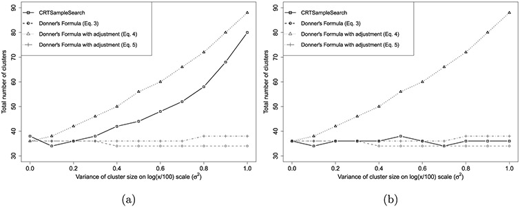
The total number of clusters needed when the size of clusters are generated from a log-Normal in Simulation 6.1. (a) Estimand (13), (b) Estimand (14).

One reason for the large differences in the required number of clusters observed for CRTsampleSearch and Equation (4) compared to Equations (3) and (5) is that they rely on different test statistics. Equations (3) and (5) were derived assuming that Y_ij(W_i) = β₀ + β₁W_i + μ_i + e_ij, where ${\mu }_i\sim N(0,{\sigma }_{\mu }^2)$ and $e_{ij}\sim N(0,{\sigma }_e^2)$. Based on this model, β₁ is the estimand of the treatment effect. If ${\sigma }_{\mu }^2$ and ${\sigma }_e^2$ are known the maximum likelihood estimator for β₁ is

$$\frac{{\sum }_{i=1}^n{W}_i{c}_i{\overline{Y}}_i^{\text{obs}}}{{\sum }_{i=1}^n{W}_i{c}_i}-\frac{{\sum }_{i=1}^n(1-W_i)c_i{\overline{Y}}_i^{\text{obs}}}{{\sum }_{i=1}^n(1-W_i)c_i},$$ (14)

where $c_i=1∕({\sigma }_{\mu }^2+\frac{{\sigma }_e^2}{m_i})$ and ${\overline{Y}}_i^{\text{obs}}=\frac{{\sum }_{j=1}^{m_i}{Y}_{ij}^{\text{obs}}}{m_i}$. Using this test statistic, van Breukelen et al. [22] showed that the loss of efficiency that stems from variation in cluster sizes rarely exceeds 10%. Figure 2(b) shows the required number of clusters calculated using Equations (3)-(5) and CRTsampleSearch when the test statistic is (14). Compared to CRTsampleSearch, Equation (3) slightly underestimates the number of required clusters and Equation (5) slightly overestimates the number of required clusters as ${\sigma }_{cs}^2$ increases. This agrees with the minimal loss of efficiency that was described previously. Because (4) calculates power for a different test statistic it significantly overestimates the number of required clusters. This analysis shows that the choice of test statistic can have a significant impact on the power of a statistical test in unbalanced designs. Similar issues are presented in Section 7 with event rates.

6.2. Non-Normal continuous outcomes

Many quantitative outcomes in healthcare studies do not follow a Normal distribution. For example, facilities’ average health expenditures may follow a log-Normal distribution and patients’ expenditure may follow a zero-inflated log-Normal distribution. Some patients have zero expenditures, some patients spend small to moderate amounts, and a few patients have extremely high expenditures [33]. To represent such cases, we generate the two potential outcomes under H₀ : E(Y(0)) = E(Y(1)) from a hierarchical zero-inflated log-Normal model as follows:

$$\begin{gathered} f_{H_0}:{\mu }_i\sim \log \text{-Normal}({\gamma }_1=1,{\gamma }_2=\psi )i=1,2,\dots ,n, \\ {Y}_{ij}(0),Y_{ij}(1)\mid {\mu }_i \\ \sim \{\begin{array}{cc}\text{log-Normal}({\gamma }_1={\mu }_i,{\gamma }_2=5),\hfill & 1-p_0=0.8,\hfill \\ 0,\hfill & p_0=0.2,\hfill \end{array}\phantom{\}}j=1,2,\dots m_i\forall i. \end{gathered}$$ (15)

Here, μ_i is the expectation of the log-Normal part of Y_ij(0) and Y_ij(1) in cluster i and the corresponding variance, γ₂, is set at 10. For simplicity, we assume that m_i = 100, ∀ i ∈ {1, … , n},, p₀ = 0.2, and the effect of the treatment is constant for every individual. The potential outcomes under H_a : E(Y(0)) ≠ E(Y(1)) are generated from the following model,

$$\begin{gathered} f_{H_a}:{\mu }_i\sim \log \text{-Normal}({\gamma }_1=1,{\gamma }_2=\psi ),i=1,2,\dots ,n, \\ {Y}_{ij}(0)\mid {\mu }_i\sim \{\begin{array}{cc}\text{log-Normal}({\gamma }_1={\mu }_i,{\gamma }_2=5),\hfill & 1-p_0=0.8,\hfill \\ 0,\hfill & p_0=0.2,\hfill \end{array}\phantom{\}}j=1,2,\dots m_i\forall i, \\ {Y}_{ij}(1)=Y_{ij}(0)+1,j=1,2,\dots m_i\forall i. \end{gathered}$$ (16)

Figure 3 shows the required number clusters calculated using Equation (3), the CRTSize package and CRTsampleSearch for different values of the between cluster variance, ψ. As ψ increases, the overall variances for the control and treated groups increase. As a result, more clusters would be required to observe a significant difference in the sample means of the two arms. This trend is captured by all three methods. However, compared to CRTsampleSearch, sample sizes derived using Equation (3) and the CRTSize package increase at higher rates. This is because the ICC in Equation (3) and CRTSize is a linear function of ψ in this simulation setting (see Appendix A.1). As ψ increases while γ₁ is constant, the log-Normal distribution is more concentrated around γ₁ with some clusters having very high values. The ICC in Equation (3) only considers the between cluster variance which is heavily influenced by extreme values. With a finite number of clusters, this results in a poor approximation of the distribution of the test statistic.

Figure 3.

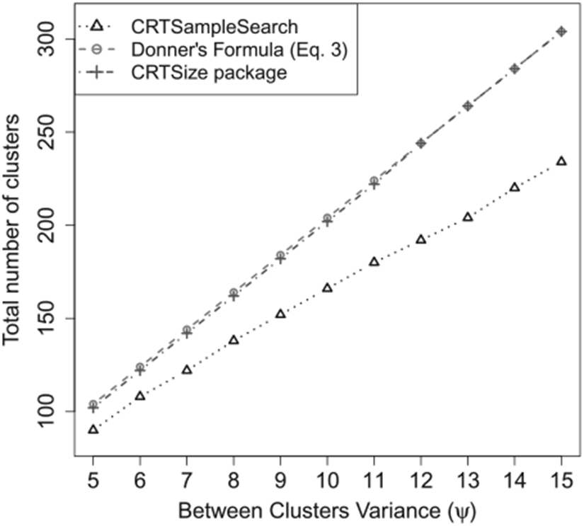
The total number of clusters needed when the outcomes are generated from a zero-inflated log-Normal model in Simulation 6.2.

When the outcome data follow a skewed distribution, other test statistics such as the difference in medians may be preferred. These statistics can be examined with the proposed simulation algorithm. However, in order to compare the proposed simulation algorithm and the currently existing formulae, we only examined Equation (13) as the test statistic.

6.3. Binary outcomes

When the outcomes are binary, the effect of the treatment is commonly estimated using the difference in proportions between the two study arms. The two potential outcomes under H₀ : E(Y(0)) = E(Y(1)) are generated from a Beta-Bernoulli model,

$$\begin{gathered} f_{H_0}:p_i\sim \text{Beta}(\alpha =1,\beta =4),i=1,2,\dots ,n, \\ {Y}_{ij}(0),Y_{ij}(1)\mid p_i\sim \mathrm{B}(p_i),j=1,2,\dots m_i\forall i. \end{gathered}$$ (17)

For simplicity, we assume that m_i = 100, ∀i ∈ {1, … , n}. The potential outcomes under H_a : E(Y(0)) ≠ E(Y(1)) are generated from the following model:

$$\begin{gathered} f_{H_a}:p_i\sim \text{Beta}(\alpha =1,\beta =4),i=1,2,\dots ,n, \\ {Y}_{ij}(0)\mid p_i\sim \mathrm{B}(p_i),j=1,2,\dots m_i\forall i, \\ {Y}_{ij}(1)\mid Y_{ij}(0),\delta \sim \mathrm{B}(\delta )(1-Y_{ij}(0))+Y_{ij}(0),j=1,2,\dots m_i\forall i. \end{gathered}$$ (18)

This f_Ha implies that the treatment only affects individuals whose outcome under the control is 0. The average effect size is $\frac{4}{5}\delta$. The test statistic is defined in Equation (13). In the context of binary outcomes, this test statistic is the difference between the proportions of successes among units in clusters with W_i = 1 and units in clusters with W_i = 0.

Figure 4 shows that the required number of clusters from CRTsampleSearch is smaller than those derived from Equation (6). This is expected because var(Y_ij(1)) > var(Y_ij(0)) under H_a (see Appendix A.2). Thus, the ICC in the treatment arm is smaller than the ICC in the control arm, while Equation (6) treats them as equal. The effect of the treatment can take any form in reality, whereas this specific simulation setting is one example in which the formulae might result in inaccurate estimations compared to CRTsampleSearch.

Figure 4.

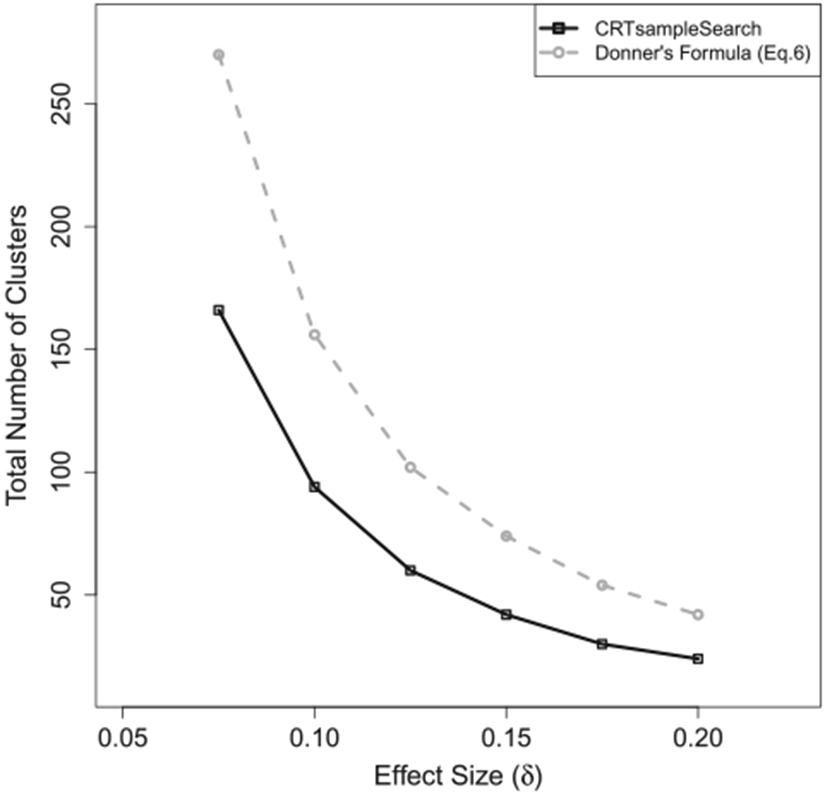
The total number of clusters needed when the outcomes are from a Beta-Bernoulli model in Simulation 6.3.

6.4. Count outcomes

Count data is commonly modelled using a Poisson distribution or a Negative Binomial distribution [34]. Equation (7) is derived assuming that the outcome follows a Poisson distribution. In some applications, the observed data include more 0 counts than expected from a Poisson or a Negative Binomial distribution. For example, the number of hospital visits in the population is a mixture of patients who do not have any visits and those that visit the hospital multiple times [33]. More appropriate models for such outcomes are the Zero-Inflated-Poisson (ZIP) or the Zero-Inflated-Negative-Binomial distribution [35]. We examined two types of data-generating mechanisms.

6.4.1. Gamma–Poisson model

The two potential outcomes under H₀ : E(Y(0)) = E(Y(1)) are generated from a Gamma–Poisson model,

$$\begin{gathered} f_{H_0}:{\lambda }_i\sim \text{Gamma}(10,2),i=1,2,\dots ,n, \\ {Y}_{ij}(0),Y_{ij}(1)\mid {\lambda }_i\sim \text{Poisson}({\lambda }_i),j=1,2,\dots m_i\forall i. \end{gathered}$$ (19)

The overall event rate under H₀ is λ₀ = 5. We assume that m_i = 100, ∈ i ∈ {1, … , n}, and that the effect of the treatment across units is δ on average. The potential outcomes under H_a : E(Y(0)) ≠ E(Y(1)) are generated from

$$\begin{gathered} f_{H_a}:{\lambda }_i\sim \text{Gamma}(10,2),i=1,2,\dots ,n, \\ {Y}_{ij}(0)\mid {\lambda }_i\sim \text{Poisson}({\lambda }_i),j=1,2,\dots m_i\forall i, \\ {Y}_{ij}(1)=Y_{ij}(0)+\text{Poisson}(\delta )j=1,2,\dots m_i\forall i. \end{gathered}$$ (20)

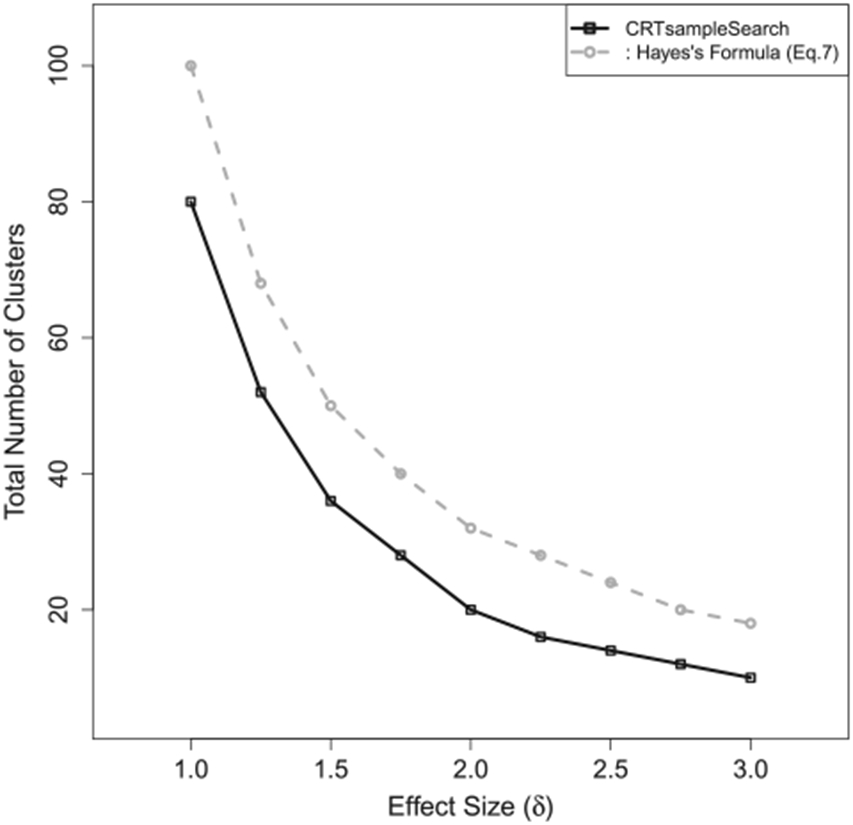
The follow-up time, t_ij, is assumed to be equal for all individuals in all of the clusters. As in the previous examples, the test statistic is defined in Equation (13). In the context of count outcomes with equal follow-up times, this statistic represents the difference between the average event rates among units in clusters with W_i = 1 and units in clusters with W_i = 0.

Figure 5 shows the required number of clusters estimated by CRTsampleSearch and Equation (7) with different effect sizes. As δ increases, the required number of clusters decreases according to both methods. Compared to the simulation-based method, Equation (7) overestimates the sample size by more than 25%.

Figure 5.

The total number of clusters needed when the outcomes are generated from a Gamma–Poisson model in Simulation 6.4.1.

6.4.2. Gamma-Zero-inflated-Poisson model

In this simulation configuration, the two potential outcomes under H₀ : E(Y(0)) = E(Y(1)) are generated from a Gamma-ZIP model,

$$\begin{gathered} f_{H_0}:{\lambda }_i\sim \text{Gamma}(10,2)i=1,2,\dots ,n, \\ {Y}_{ij}(0),Y_{ij}(1)\mid {\lambda }_i,p_0\sim \{\begin{array}{cc}\text{Poisson}({\lambda }_i),\hfill & 1-p_0,\hfill \\ 0,\hfill & p_0,\hfill \end{array}\phantom{\}}j=1,2,\dots m_i\forall i. \end{gathered}$$ (21)

The overall event rate under H₀ is λ₀ = 5(1 – p₀). We assume that m_i = 100, ∀i ∈ {1, … , n}, and that the effect of the treatment across units is δ = 1 on average. The potential outcomes under H_a : E(Y(0)) ≠ E(Y(1)) are generated from the following model:

$$\begin{gathered} f_{H_a}:{\lambda }_i\sim \text{Gamma}(10,2),i=1,2,\dots ,n, \\ {Y}_{ij}(0)\mid {\lambda }_i,p_0\sim \{\begin{array}{cc}\text{Poisson}({\lambda }_i),\hfill & 1-p_0,\hfill \\ 0,\hfill & p_0,\hfill \end{array}\phantom{\}}j=1,2,\dots m_i\forall i, \\ {Y}_{ij}(1)=Y_{ij}(0)+\text{Poisson}(\delta =1),j=1,2,\dots m_i\forall i. \end{gathered}$$ (22)

The follow-up time, t_ij, is assumed to be equal for all individuals in all clusters, and the test statistic is defined in Equation (13). Figure 6 presents the required number of clusters estimated by CRTsampleSearch and Equation (7). As p₀ increases, the required number of clusters decreases according to both methods. Compared to the simulation-based method, Equation (7) overestimates the sample size by more than 24%.

Figure 6.

The total number of clusters needed when the outcomes are generated from a Gamma-ZIP model in Simulation 6.4.2.

7. Real data example: hospitalization count in nursing homes

In many practical situations, researchers have prior information on their study population and the expected effect size. For example, data or summary statistics from previous studies provide information on the distributions of the potential outcomes in the control arms. We implement the proposed simulation-based approach using hospitalization data collected from a CRT performed in US nursing homes during the flu season of 2013–2014 [36] and compare it with MLPowSim [8].

The flu vaccine data comprise 817 nursing homes and 52,964 patients. We removed patients with less than 10 days of follow-up and nursing homes with fewer than 10 patients because they may suffer from very high hospitalization rates. Including these patients and nursing homes results in large sampling variances and a large number of required clusters. As a consequence, a CRT of this size is financially and logistically impractical.

After removing patients with less than 10 days of follow-up time and nursing homes with less than 10 patients, there are 814 nursing homes and 52,522 patients. The number of patients enrolled in each cluster varies from 14 to 492 with an average of 65 patients per nursing home Figure 7. Each nursing home accumulated 34 person-years on average. The average patient-level hospitalization rate, $({\sum }_{i,j}\frac{Y_{ij}^{\text{obs}}}{t_{ij}})∕({\sum }_i{m}_i)$, is 0.74 per person-year. The average cluster-level pooled hospitalization rate, $({\sum }_i\frac{{\sum }_j{Y}_{ij}^{\text{obs}}}{{\sum }_j{t}_{ij}})∕n$, is 0.56 per person-year. The pooled hospitalization rate, $({\sum }_{i,j}{Y}_{ij}^{\text{obs}})∕({\sum }_{i,j}{t}_{ij})$, is 0.55 per person-year. Table 1 presents the individual-level hospitalization rates. It is heavily inflated at 0 compared to a Poisson distribution with a rate of 0.55. Approximately 80% of the patients never experienced any hospitalization during their follow-up time. Figure 8 shows the ZIP model estimates from each of the nursing homes. The proportions of zeros in the binary component vary from 0 to 1 with a mean of 0.71 Figure 8(a). The event rates in the Poisson component range from 0 to 4 per person-year in most nursing homes except for a few with rates over 12 per person-year Figure 8(b).

Figure 7.

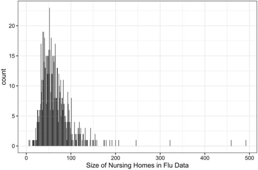
The size of nursing homes recruited in the influenza study.

Table 1.

Distribution of individual-level hospitalization rate (λ, count/year) in the flu vaccine data.

λ	0	(0,3]	(3,5]	(5,10]	(10,50]	(50, 60.875]
Counts	41818	6315	2251	1587	550	2
Percent	79.620	12.023	4.286	3.020	1.047	0.004

Figure 8. Estimations from the ZIP(P₀, λ₀) model for every nursing homes in the flu vaccine data.

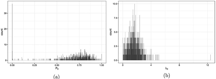
Note: (a) The proportion of zeros (P₀) in the binary component. (b) The event rate (λ₀) in the Poisson component.

7.1. Number of clusters required for a new CRT

7.1.1. Data generating and sampling mechanisms

If a new CRT study will be performed on a similar population, the flu vaccine data provide a reasonable approximation for the distribution of cluster sizes and the potential outcomes in the control arm. Formally, a new CRT with n clusters can be simulated from the following model:

$$\begin{gathered} f_0:I{D}_i\sim f(x)\propto 1∕814,x\in \{1,2,\dots ,814\}, \\ {m}_i=\text{Size of cluster}I{D}_i\text{in the flu vaccine data}, \\ {Y}_{ij}(0)=\text{Counts observed for subject}j\text{in cluster}I{D}_i\text{in the flu vaccine data}, \\ {t}_{ij}(0)=\text{Follow-up time observed for subject}j\text{in cluster}I{D}_i\text{in the flu vaccine data}, \\ j=1,2,\dots ,m_i,i=1,2,\dots ,n. \end{gathered}$$ (23)

Denote Model (23) as $f_0^{\text{Flu-Vaccine}}$. Under the null hypothesis, we assume that Y_ij(1) = Y_ij(0) and t_ij(1) = t_ij(0) ∀i, j, where t_ij(w) is the follow-up time for patient j in cluster i if the cluster is assigned to treatment w. Both Neyman’s null and Fisher’s null are valid under this data generating model.

One possible data generating mechanism under H_a is that the treatment is expected to reduce the hospitalization rate component by 0.5

$$\begin{gathered} H_a^{\text{Poisson}}:Y_{ij}(0)\sim f_0^{\text{Flu-Vaccine}}, \\ {Y}_{ij}(1)\sim \text{Poisson}\left(\max \{0,{\lambda }_{ij}(0)-0.5\}{t}_{ij}(1)\right), \\ {t}_{ij}(1)=t_{ij}(0), \\ \text{where}{\lambda }_{ij}(0)=Y_{ij}(0)∕t_{ij}(0),j=1,2,\dots m_i,i=1,2,\dots ,n. \end{gathered}$$ (24)

A different possible data generating mechanism under H_a assumes that the new treatment would only reduce the number of hospitalizations for nursing home residents who would experience hospitalizations in the control arm. For this data generating model, the potential outcomes under H_a are generated from

$$\begin{gathered} H_a^{\text{ZIP}}:Y_{ij}(0)\sim f_0^{\text{Flu-Vaccine}}, \\ {Y}_{ij}(1)\sim \text{ZIP}\left(P_0^i,\max \{0,{\lambda }_0^i-0.1\}{t}_{ij}(1)\right), \\ {t}_{ij}(1)=t_{ij}(0),j=1,2,\dots m_i,i=1,2,\dots ,n, \end{gathered}$$ (25)

where $P_0^i$ is the estimated proportion of inflation at 0 for nursing home i and ${\lambda }_0^i$ is the estimated event rate for nursing home i in the ZIP model, which is defined similarly to Equation (21) with $p_0=P_0^i$ and ${\lambda }_i=\max \{0,{\lambda }_0^i-0.1\}{t}_{ij}(1)$ for subjects in cluster i.

The race of patients is known to be correlated with the hospitalizations rates [37]. Another possible data generating mechanism under H_a assumes that the new treatment will reduce the number of hospitalizations for African American nursing home residents less than residents from other race groups. For this data generating model, the potential outcomes under $H_a^{Race}$ can be generated from

$$\begin{gathered} H_a^{\text{Race}}:Y_{ij}(0)\sim f_0^{\text{Flu-Vaccine}}, \\ {Y}_{ij}(1)\sim \text{Poisson}\left(\max \{0,{\lambda }_{ij}(0)-0.4-0.1A_{ij}\}{t}_{ij}(1)\right), \\ {t}_{ij}(1)=t_{ij}(0),j=1,2,\dots m_i,i=1,2,\dots ,n, \end{gathered}$$ (26)

where A_ij = 1 if patient j in nursing home i is not African American and A_ij = 0 otherwise, and ${\lambda }_{ij}(0)=\frac{Y_{ij}(0)}{t_{ij}(0)}$, ∀i = 1, 2, … , n, j = 1, 2, … m_i.

7.1.2. Randomization mechanisms

Complete randomization.

If the treatment is assigned completely at random in a new CRT, then the assignment indicator at the nursing home level can be generated from f(W ∣ X) : $W_i\sim \text{Bernoulli}(\frac{1}{2})$, i = 1, 2, …, n such that ${\sum }_i^n{W}_i=\frac{n}{2}$ for balanced study design.

Stratified randomization.

Stratified randomization has been proposed as a technique to balance pre-treatment characteristics of participating clusters and increase power [38]. In the flu vaccine data, the proportions of African American residents vary across different nursing homes as shown in Figure 9. A new CRT may balance the number of African Americans across study arms using stratified randomization. Let X_i be the proportion of African American residents in nursing home i, the assignment indicator at the nursing home level will be generated from $f(W\mid X):W_i\mid X_i\in s\sim \text{Bernoulli}(\frac{1}{2})$ where s ∈ {[Q₀, Q₁], (Q₁, Q₂], (Q₂, Q₃], (Q₃, Q₄]} and Q_q is the q th quartile of X_i. These partitions are nursing homes into distinct groups by the quartiles of the observed proportions of African American residents in the nursing homes.

Figure 9. The percentage of African American residents per nursing home in the flu vaccine data.

Note: Stratum 1: ≤ 1.47% (204 nursing homes, 25.06% of the total); stratum 2: (1.47%, 6.25%] (204 nursing homes, 25.06% of the total); stratum 3: (6.25%, 17.9%] (204 nursing homes, 25.06% of the total); stratum 4: > 17.9% (202 nursing homes, 24.82% of the total).

7.1.3. Test statistics

Difference in hospitalization rates.

Equation (7) assumes that the population rates in the control and treatment arms are λ₀ and λ₁, respectively. When clusters and units within clusters contribute an equal amount of time, λ_i can be approximated by averaging unit level rates, $({\sum }_{i,j}\frac{Y_{ij}^{\text{obs}}}{t_{ij}^{\text{obs}}})∕(\sum m_i)$, or by the pooled rates, $({\sum }_{i,j}{Y}_{ij}^{\text{obs}})∕({\sum }_{i,j}{t}_{ij}^{\text{obs}})$, where $t_{ij}^{\text{obs}}=t_{ij}(1)W_i+t_{ij}(0)(1-W_i)$. This equivalence in estimates does not hold when the time contributed by each unit is different. Because CRTsampleSearch requires to explicitly define the test statistic we estimated both the difference between the pooled rates and the difference between the average unit-level rates.

Treatment effect estimated from Hierarchical models.

Hierarchical models have been proposed to estimate the effects of intervention in CRTs [39]. Generalized Linear Mixed Effect Model (GLMM) estimates the effect of the treatment while adjusting for clustering at the second level. When using GLMM, the test statistic, T, is the estimated coefficient corresponding to the treatment assignment indicator.

7.1.4. Required number of clusters

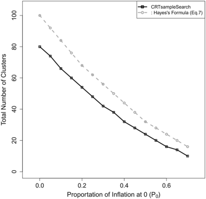
Assuming a significance level of 0.05 and minimal power of 0.8, Table 2 summarizes results from Hayes’s formula, MLPowSim, and CRTsampleSearch for the data generating mechanisms described in Equations (24)-(26). For the data generating mechanisms in Equations (24) and (26), when the difference in the pooled event rates between the two study arms is the test statistic, the minimal number of clusters estimated by CRTsampleSearch are 11% to 40% larger than those estimated using Equation (7). This is because Equation (7) ignores the variability in patients’ follow-up time accumulated by each nursing home. When the difference in the average patient-level event rates between the two study arms is the test statistic, CRTsampleSearch results in a significantly larger number of required clusters than Equation (7). This is because the variation of patient-level event rate is bigger than the pooled event rate in each study arm. When using the treatment effect estimated from a GLMM model, CRTsampleSearch results in a larger number of required clusters compared to MLPowSim. This is because MLPowSim assumes that all nursing homes would enroll the same number of patients and every patient would be followed for the same amount of time. For the data generating model in Equation (25), CRTsampleSearch results in fewer clusters than Equation (6) when the difference in average patient-level event rates between the two study arms is the test statistic. The data generating model in Equation (25) assumes that Y_ij(1) is independent from Y_ij(0) given the clusters’ data generating parameters. The correlation between Y_ij(1) and Y_ij(0) is much smaller than the data generating models in Equations (24) and (26). Under $H_a^{\text{ZIP}}$, the pooled event rate and patient-level event rate in the treatment arm are both around 0.36 times per person year. However, under H₀, the pooled event rate is around 0.55 times per person year, while the patient-level event rate is around 0.74 times per person year.

Table 2.

The total number of clusters required (N) to test the Neyman’s null H₀ : E(Y(0)) = E(Y(1)) against three different H_a using Equation (7), MLPowSim and CRTsampleSearch.

			MLPowSim				CRTsampleSearch
	Equation (7) a		β2 = 0b		β2 = 0.23c		Complete randomization			Stratified randomization
Y(1)	λ 1	N	β 1	N	β 1	N	A	B	C	A	B	C
$H_a^{\text{Poisson}}$	0.460	224	−0.2087	164	−0.2089	156	292	586	184	274	560	176
$H_a^{\text{Race}}$	0.464	242	−0.2003	178	−0.2005	170	314	640	196	298	604	190
$H_a^{\text{ZIP}}$	0.362	50	−0.4825	32	−0.4830	30	68	36	44	64	34	38

Notes: MLPowSim fits a 2-level regression model Y_ij ~ Poisson(λ_ij) and log(λ_ij) = β₀ + β₁W_ij + β₂X_ij + z_i where $z_i\sim \mathcal{N}(0,{\sigma }_z^2)$ and W_ij = W_ik ∀i, j ≠ k assuming equal size of clusters as 65. CRTsampleSearch (A) uses the difference in the pooled event rates in the two study arms as the test statistic; (B) uses the difference in the average person-level event rates in the two study arms as the test statistic; (C) uses the treatment effect estimated from a GLMM model as the test statistic; Stratified randomization uses the percentage of African American in nursing homes to define the strata.

^aλ₀ = 0.557, $\overline{v}=33.86$ and CV_B = 0.442.

^bWith no extra covariate. β₀ = −0.68 and ${\sigma }_u^2=0.19$.

^cIncludes patient-level indicator for African American as the extra covariate. β₀ = −0.71 and ${\sigma }_u^2=0.18$.

For all three types of data-generating models in Equations (24)-(26), MLPowSim adjusted for an indicator for individual’s race resulted in a smaller number of required samples. Similarly, using stratified randomization with CRTsampleSearch resulted in a smaller number of required clusters compared to complete randomization. However, while the estimand used in CRTsampleSearch for the different randomization procedures is the same, the estimands obtained from MLPowSim are different.

7.2. Finite population of clusters

The flu vaccine data provides information on 814 nursing homes, which is generally considered a large trial. In other trials, the population of interest may comprise a subset of these 814 nursing homes. We selected a random sample of 16 nursing homes from the flu vaccine data and assume that they represent the entire population of nursing homes in a new CRT. When the population of clusters is infinite, the data generating and recording mechanisms should sample with replacement from these 16 nursing homes. When the population is finite, the data generating and recording mechanisms should sample without replacement from these 16 nursing homes. In addition, when the number of nursing homes is small, a permutation test at the cluster level might be more appropriate than asymptotic approximations.

Table 3 presents the power estimated using CRTsampleSearch under Neyman’s null and under Fisher’s null using a permutation test when the population is either infinite or finite. The test statistic is the difference in the pooled hospitalization rates between the two study arms. The potential outcomes are generated under $H_a^{\text{Poisson}}$. Generally, the permutation test for Fisher’s null is more powerful than the test for Neyman’s null because Fisher’s null is more conservative than Neyman’s null. The differences in statistical power generally decrease with an increasing number of clusters in the population. The powers of both tests are similar when sampling is performed without replacement and the number of sampled clusters equals the number of clusters in the population. This result is expected because inferences under the two null hypotheses are often asymptotically similar for the difference in expectations [30].

Table 3.

The power testing Neyman’s null and Fisher’s null against $H_a^{\text{Poisson}}$ using a random subset of 16 nursing homes from the flu vaccine data.

	Sample WITHOUT replacement		Sample WITH replacement
N a	Neyman’s null	Fisher’s null	Neyman’s null	Fisher’s null
10	0.147	0.177	0.132	0.205
12	0.167	0.185	0.150	0.207
14	0.185	0.195	0.168	0.218
16	0.207	0.206	0.188	0.233
18			0.204	0.250
20			0.222	0.270

Notes: The test statistic is the difference in the pooled hospitalization rates between the two arms and randomization mechanism is complete randomization.

^aThe total number of clusters in the CRT.

8. Discussion

We propose a new simulation-based approach for estimating the minimum number of required clusters to identify an effect size for a predefined statistical power for CRTs. The simulation procedure is defined using the potential outcome framework, which allows for an explicit definition of the data generating, recording, and treatment assignment mechanisms. By explicitly defining the data generating mechanism, researchers can examine the power of any null and alternative hypotheses. Using real data, we demonstrated that the power under Neyman’s and Fisher’s null hypotheses can differ even when the same test statistic is used.

Most formulae and simulation-based algorithms for sample size estimation in CRT ignore the treatment assignment mechanism and concentrate on the data generating mechanism. Our proposed algorithm enables the examination of different assignment mechanisms. We provide examples for implementing complete randomization and stratified randomization. Other randomization schemes can be easily implemented as well.

Another key feature that sets the proposed approach apart from existing sample size estimation methods for CRTs is that the proposed approach allows for the definition of any test statistic and it does not rely on the asymptotic approximation of the distribution of the test statistic to calculate statistical power. When the number of clusters, as well as the sizes of clusters, are large and the test statistic is the difference in means or maximum likelihood-based estimators, the asymptotic approximations are generally accurate. However, when the number of clusters is small or when the outcomes do not follow standard distributions, these asymptotic approximations may not be accurate and result in over or underestimation of the minimal required number of clusters. This was shown with simulated data as well as data from a CRT. The proposed procedure also enables the estimation of the required sample size for permutation tests. For these tests, asymptotic approximations can be complex to derive analytically for different statistics.

When using previously collected data, one should ensure that the collected data represent the population that the new intervention would be applied to. For example, because of recording errors or censoring, outliers may exist in previously collected data. In a new study, these may not exist or the analysis would be limited only to specific individuals. Including outliers in sample size calculations may result in a large sampling variance, which would require a large number of clusters to reach a prespecified power.

To take full advantage of the simulation-based approach, researchers should provide the cluster size distribution, the data generating model, the randomization distribution and the test statistics. However, researchers can still gain important insights on the required sample size when only some of these mechanisms are known. The test statistic is defined by the researchers and it should be selected based on the scientific question and the intended audience of the results, and not only its statistical properties. Information on the cluster-size distribution is commonly available from previous data and can be incorporated into the proposed simulation-based approach. If applicable, multiple randomization schemes should be considered at the design stage to identify the ones that are most efficient. The data generating distribution may suffer from limited information in some applications. In such cases, researchers should examine several plausible mechanisms in order to identify the effects of the different mechanisms. Some of these mechanisms can be similar to the ones assumed by the analytically derived formulae. Results based on deviations from the analytical formulae can inform researchers regarding the possible need for a different number of required clusters to ensure sufficient power when the assumed mechanisms are misspecified.

Simulation-based approaches are computationally intensive compared to analytically derived sample size formulae, which may impede their use in practice [9]. Moreover, the proposed simulation approach requires some programming knowledge to implement. To address these limitations, an R package CRTsampleSearch is developed. The package relies on the binary search algorithm and parallel computing to reduce the computational burden. In addition, we provide code examples to ease implementation (https://ruoshuiaqua.github.io/CRTsampleSearchExamples.io/).

In conclusion, we describe a flexible simulation-based algorithm to estimate the minimal number of clusters that are required to identify an effect in CRTs for a specified power. The procedure can rely on summary statistics, hypothetical distributions, or previously collected data to approximate the required optimal number of clusters for a new CRT.

Appendix 1. Additional material

A.1. Zero-inflated log-Normal model in Section 6.2

Under H₀ and H_a, the total variance of the potential outcome Y_ij(0):

$${\sigma }_T^2=\text{var}\left(Y_{ij}(0)\right)=E\left\{\text{var}\left(Y_{ij}(0)\mid {\mu }_i,p_0\right)\right\}+\text{var}\left\{E\left(Y_{ij}(0)\mid {\mu }_i,p_0\right)\right\},$$

where p₀ is the inflation parameter and μ_i is the expectation of the log-Normal part of Y_ij (0)’s distribution as defined in Equation (15). We assume that μ_i ~ log-Normal(γ₁ = η₀, ψ) and we denote the variance of the log-Normal part of Y_ij(0)’s distribution as γ₂. In Equation (15), η₀ = 1. The total variance of Y_ij(0) is

$$\begin{gathered} \text{var}\left(Y_{ij}(0)\mid {\mu }_i,p_0\right)=E\left(Y_{ij}^2(0)\mid {\mu }_i,p_0\right)-E^2\left(Y_{ij}(0)\mid {\mu }_i,p_0\right) \\ =(1-p_0)({\gamma }_2+{\mu }_i^2)-(1-p_0{)}^2{\mu }_i^2 \\ =(1-p_0){\gamma }_2+p_0(1-p_0){\mu }_i^2, \\ E\left(Y_{ij}(0)\mid {\mu }_i,p_0\right)=(1-p_0){\mu }_i. \end{gathered}$$

Therefore,

$$\begin{gathered} {\sigma }_T^2=E((1-p_0){\gamma }_2+p_0(1-p_0){\mu }_i^2)+\text{var}((1-p_0){\mu }_i) \\ =(1-p_0){\gamma }_2+p_0(1-p_0)({\eta }_0^2+\psi )+(1-p_0{)}^2\psi \\ ={\gamma }_2+\psi -{\eta }_0^2{p}_0^2-({\gamma }_2+\psi -{\eta }_0^2)p_0. \end{gathered}$$

The between cluster variance is var(E(Y_ij(0) ∣ μ_i, p₀)) = (1 – p₀)²ψ, and the ICC in this model is $\rho =(1-p_0{)}^2\psi ∕{\sigma }_T^2$. Estimation for the required number of clusters using Equation (3) is

$$\frac{n}{2}=\frac{2{\sigma }_T^2(Z_{\alpha ∕2}+Z_{\beta }{)}^2(1+(m-1)\rho )}{m{\delta }^2}\propto \psi$$

when α, β, m, p₀, γ₂, η₀ and δ are fixed in these simulations.

A.2. Beta-Bernoulli model in Section 6.3

Under H₀ and H_a, the total variance of the potential outcome Y_ij(0) is:

$$\begin{gathered} \text{var}\left(Y_{ij}(0)\right)=E\left\{\text{var}\left(Y_{ij}(0)\mid p_i\right)\right\}+\text{var}\left\{E\left(Y_{ij}(0)\mid p_i\right)\right\} \\ =E(p_i(1-p_i))+\text{var}(p_i) \\ =E(p_i)-E(p_i^2)+\text{var}(p_i) \\ =E(p_i)-E^2(p_i) \\ =\frac{\alpha \beta }{(\alpha +\beta {)}^2}. \end{gathered}$$

This is the same as the total variance of the potential outcome Y_ij(1) under H₀. Hence, ICC in the control arm under H₀ and H_a and ICC in the treatment are under H₀ all equal to $\frac{\text{var}(p_i)}{\text{var}\left(Y_{ij}(0)\right)}=\frac{1}{\alpha +\beta +1}=\frac{1}{6}$.

Under H_a, the total variance of the potential outcome Y_ij(1) is

$$\begin{gathered} \text{var}\left(Y_{ij}(1)\right)=E\left\{\text{var}\left(Y_{ij}(1)\mid \delta ,p_i\right)\right\}+\text{var}\left\{E\left(Y_{ij}(1)\mid \delta ,p_i\right)\right\} \\ =E\left\{E\left(Y_{ij}(1{)}^2\mid \delta ,p_i\right)-E^2\left(Y_{ij}(1)\mid \delta ,p_i\right)\right\}+\text{var}\left\{E(\delta (1-Y_{ij}(0))+Y_{ij}(0)\mid p_i)\right\} \\ =E\left\{E(Y_{ij}(1)\mid \delta ,p_i)-E^2(Y_{ij}(1)\mid \delta ,p_i)\right\}+\text{var}(\delta +(1-\delta )p_i) \\ =E\left\{\delta +(1-\delta )p_i-(\delta +(1-\delta )p_i{)}^2\right\}+(1-\delta {)}^2\text{var}(p_i) \\ =\delta +(1-\delta )E(p_i)-{\delta }^2-2\delta (1-\delta )E(p_i)-(1-\delta {)}^{2}E(p_i^2)+(1-\delta {)}^2\text{var}(p_i) \\ =\delta -{\delta }^2+(1-\delta )(1-2\delta )E(p_i)-(1-\delta {)}^2{E}^2(p_i) \\ =\delta -{\delta }^2-\delta (1-\delta )E(p_i)+(1-\delta {)}^{2}E(p_i)-(1-\delta {)}^2{E}^2(p_i) \\ =\delta (1-\delta )(1-E(p_i))+(1-\delta {)}^2\text{var}\left(Y_{ij}(0)\right). \end{gathered}$$

And the between cluster variance is

$$\text{var}\left\{E\left(Y_{ij}(1)\mid \delta ,p_i\right)\right\}=(1-\delta {)}^2\text{var}(p_i).$$

Hence, ICC in the treatment arm under H_a is $\frac{\text{var}\left\{E\left(Y_{ij}(1)\mid \delta ,p_i\right)\right\}}{\text{var}\left(Y_{ij}(1)\right)}=\frac{\text{var}(p_i)}{\frac{\delta }{1-\delta }\left(1-E(p_i)\right)+\text{var}\left(Y_{ij}(0)\right)}<\frac{1}{6}$ when δ ∈ (0, 1)

References

- [1].Moberg J, Kramer M. A brief history of the cluster randomised trial design. J R Soc Med. 2015;108(5):192–198. [DOI] [PMC free article] [PubMed] [Google Scholar]
- [2].Donner A, Klar N. Design and analysis of cluster randomization trials in health research. London: Arnold; 2000. [Google Scholar]
- [3].Donner A, Klar N. Pitfalls of and controversies in cluster randomization trials. Am J Public Health. 2004;94(3):416–422. [DOI] [PMC free article] [PubMed] [Google Scholar]
- [4].Rotondi MA, Donner A. Sample size estimation in cluster randomized educational trials: an empirical Bayes approach. J Educ Behav Stat. 2009;34(2):229–237. [Google Scholar]
- [5].Hayes RJ, Bennett S. Simple sample size calculation for cluster-randomized trials. Int J Epidemiol. 1999;28(2):319–326. [DOI] [PubMed] [Google Scholar]
- [6].Rotondi MA. CRTSize: sample size estimation functions for cluster randomized trials; 2015. R package version 1.0. Available from: https://CRAN.R-project.org/package=CRTSize. [Google Scholar]
- [7].Rutterford C, Copas A, Eldridge S. Methods for sample size determination in cluster randomized trials. Int J Epidemiol. 2015;44(3):1051–1067. [DOI] [PMC free article] [PubMed] [Google Scholar]
- [8].Browne WJ, Lahi MG, Parker RMA. A guide to sample size calculations for random effect models via simulation and the MLPowSim software package. Bristol (UK): University of Bristol; 2009. [Google Scholar]
- [9].Hooper R Versatile sample-size calculation using simulation. Stata J. 2013;13(1):21–38. [Google Scholar]
- [10].Kleinman K, Huang SS. Calculating power by bootstrap, with an application to cluster-randomized trials. eGEMs. 2016;4(1):1202. [DOI] [PMC free article] [PubMed] [Google Scholar]
- [11].Lohr SL. Sampling: design and analysis: design and analysis. Boca Raton: Chapman and Hall/CRC; 2019. [Google Scholar]
- [12].Rosenberger WF, Lachin JM. Randomization in clinical trials: theory and practice. New York: John Wiley & Sons; 2015. [Google Scholar]
- [13].Cook AJ, Delong E, Murray DM, et al. Statistical lessons learned for designing cluster randomized pragmatic clinical trials from the NIH health care systems collaboratory biostatistics and design core. Clinical Trials. 2016;13(5):504–512. [DOI] [PMC free article] [PubMed] [Google Scholar]
- [14].Imbens GW, Rubin DB. Causal inference in statistics, social, and biomedical sciences. New York: Cambridge University Press; 2015. [Google Scholar]
- [15].Rubin DB. Comment. J Am Stat Assoc. 1980;75(371):591–593. [Google Scholar]
- [16].Rubin DB. 2 statistical inference for causal effects, with emphasis on applications in epidemiology and medical statistics. Handbook Stat. 2007;27:28–63. [Google Scholar]
- [17].Rubin DB. Bayesian inference for causal effects: the role of randomization. Ann Stat. 1978;6:34–58. [Google Scholar]
- [18].Donner A, Birkett N, Buck C. Randomization by cluster: sample size requirements and analysis. Am J Epidemiol. 1981;114(6):906–914. [DOI] [PubMed] [Google Scholar]
- [19].van Breukelen GJP, Candel MJJM. How to design and analyse cluster randomized trials with a small number of clusters? Comment on Leyrat et al. Int J Epidemiol. 2018;47(3):998–1001. [DOI] [PubMed] [Google Scholar]
- [20].Lauer SA, Kleinman KP, Reich NG. The effect of cluster size variability on statistical power in cluster-randomized trials. PLoS ONE. 2015;10(4):e0119074. [DOI] [PMC free article] [PubMed] [Google Scholar]
- [21].Manatunga AK, Hudgens MG, Chen S. Sample size estimation in cluster randomized studies with varying cluster size. Biom J. 2001;43(1):75–86. [Google Scholar]
- [22].van Breukelen GJP, Candel MJJM, Berger MPF. Relative efficiency of unequal versus equal cluster sizes in cluster randomized and multicentre trials. Stat Med. 2007;26(13):2589–2603. [DOI] [PubMed] [Google Scholar]
- [23].Ridout MS, Demetrio CGB, Firth D. Estimating intraclass correlation for binary data. Biometrics. 1999;55(1):137–148. [DOI] [PubMed] [Google Scholar]
- [24].Wu S, Crespi CM, Weng KW. Comparison of methods for estimating the intraclass correlation coefficient for binary responses in cancer prevention cluster randomized trials. Contemp Clin Trials. 2012;33(5):869–880. [DOI] [PMC free article] [PubMed] [Google Scholar]
- [25].StataCorp. Stata statistical software: release 16. College Station (TX): StataCorp LLC; 2019. [Google Scholar]
- [26].Gail MH, Mark SD, Carroll RJ, et al. On design considerations and randomization-based inference for community intervention trials. Stat Med. 1996;15(11):1069–1092. [DOI] [PubMed] [Google Scholar]
- [27].Small DS, Ten Have TR, Rosenbaum PR. Randomization inference in a group–randomized trial of treatments for depression: covariate adjustment, noncompliance, and quantile effects. J Am Stat Assoc. 2008;103(481):271–279. [Google Scholar]
- [28].Wang R, De Gruttola V. The use of permutation tests for the analysis of parallel and stepped-wedge cluster-randomized trials. Stat Med. 2017;36(18):2831–2843. [DOI] [PMC free article] [PubMed] [Google Scholar]
- [29].Kempthorne O, Hinkelmann K. Design and analysis of experiments. Vol. 1: Introduction to Experimental Design. Hoboken, NJ: Wiley; 2007. [Google Scholar]
- [30].Rosenbaum PR. Observational studies. New York: Springer; 2010. [Google Scholar]
- [31].Ding P et al. A paradox from randomization-based causal inference. Stat Sci. 2017;32(3): 331–345. [Google Scholar]
- [32].Flores I, Madpis G. Average binary search length for dense ordered lists. Commun ACM. 1971;14(9):602–603. [Google Scholar]
- [33].Steiner C, Elixhauser A, Schnaier J. The healthcare cost and utilization project: an overview. Eff Clin Pract. 2002;5(3):143–151. [PubMed] [Google Scholar]
- [34].Cameron AC, Trivedi PK. Regression analysis of count data. Vol. 53. Cambridge, United Kingdom: Cambridge University Press; 2013. [Google Scholar]
- [35].Zuur AF, Ieno EN, Walker NJ, et al. Zero-truncated and zero-inflated models for count data. Mixed effects models and extensions in ecology with R. New York, NY: Springer; 2009. p. 261–291. [Google Scholar]
- [36].Gravenstein S, Davidson HE, Taljaard M, et al. Comparative effectiveness of high-dose versus standard-dose influenza vaccination on numbers of us nursing home residents admitted to hospital: a cluster-randomised trial. Lancet Respir Med. 2017;5(9):738–746. [DOI] [PubMed] [Google Scholar]
- [37].Schulz AJ, Ed Mullings L. Gender, race, class, & health: intersectional approaches. San Francisco, CA: Jossey-Bass; 2006. [Google Scholar]
- [38].Kernan WN, Viscoli CM, Makuch RW, et al. Stratified randomization for clinical trials. J Clin Epidemiol. 1999;52(1):19–26. [DOI] [PubMed] [Google Scholar]
- [39].Raudenbush SW. Statistical analysis and optimal design for cluster randomized trials. Psychol Meth. 1997;2(2):173–185. [DOI] [PubMed] [Google Scholar]