Assessing the Trustworthiness of Saliency Maps for Localizing Abnormalities in Medical Imaging

Abstract

Purpose

To evaluate the trustworthiness of saliency maps for abnormality localization in medical imaging.

Materials and Methods

Using two large publicly available radiology datasets (Society for Imaging Informatics in Medicine–American College of Radiology Pneumothorax Segmentation dataset and Radiological Society of North America Pneumonia Detection Challenge dataset), the performance of eight commonly used saliency map techniques were quantified in regard to (a) localization utility (segmentation and detection), (b) sensitivity to model weight randomization, (c) repeatability, and (d) reproducibility. Their performances versus baseline methods and localization network architectures were compared, using area under the precision-recall curve (AUPRC) and structural similarity index measure (SSIM) as metrics.

Results

All eight saliency map techniques failed at least one of the criteria and were inferior in performance compared with localization networks. For pneumothorax segmentation, the AUPRC ranged from 0.024 to 0.224, while a U-Net achieved a significantly superior AUPRC of 0.404 (P < .005). For pneumonia detection, the AUPRC ranged from 0.160 to 0.519, while a RetinaNet achieved a significantly superior AUPRC of 0.596 (P <.005). Five and two saliency methods (of eight) failed the model randomization test on the segmentation and detection datasets, respectively, suggesting that these methods are not sensitive to changes in model parameters. The repeatability and reproducibility of the majority of the saliency methods were worse than localization networks for both the segmentation and detection datasets.

Conclusion

The use of saliency maps in the high-risk domain of medical imaging warrants additional scrutiny and recommend that detection or segmentation models be used if localization is the desired output of the network.

Keywords: Technology Assessment, Technical Aspects, Feature Detection, Convolutional Neural Network (CNN)

Supplemental material is available for this article.

© RSNA, 2021

Summary

A variety of saliency map techniques used to interpret deep neural networks trained on medical imaging did not pass several key criteria for utility and robustness, highlighting the need for additional validation before clinical application.

Key Points

• ■ Eight popular saliency map techniques were evaluated for their utility and robustness in interpreting deep neural networks trained on chest radiographs.

• ■ All the saliency map techniques did not pass at least one of the criteria that had been defined in the original study, indicating their use for high-risk medical applications to be problematic. In particular, only XRAI passed the localization utility test for both the segmentation and detection datasets (segmentation, P = .02; detection, P < .001), but it did not pass the randomization test for both datasets (P < .001). Moreover, no saliency method was found to be more repeatable or reproducible than their localization network counterpart (P < .001), with XRAI repeatability on the detection dataset being the sole exception in the detection dataset (P < .001).

• ■ The use of detection or segmentation models is recommended if localization is the ultimate goal of interpretation. These models outperformed all eight saliency methods in terms of localization utility on both the detection and segmentation datasets (P < .001).

Introduction

Deep learning has brought many promising applications within medical imaging, with recent studies showing potential for key clinical assessments within radiology (1–3). One major class of deep neural networks is convolutional neural networks (CNNs), which take raw pixel values as input and transform them into the output of interest (such as diagnosis). Many CNNs have outperformed conventional methods for various medical tasks (4,5). As CNNs are becoming popular for classification of medical images, it has become important to find methods that explain the decisions of these models to establish trust with clinicians. Saliency maps have become a popular approach for post hoc interpretability of CNNs. These maps are designed to highlight the salient components of medical images that are important to model prediction. As a result, many CNN medical imaging studies have used saliency maps to rationalize model prediction and provide localization (6–8). However, a recent study that evaluated a variety of datasets showed that many popular saliency maps are not sensitive to model weight or label randomization (6). Although, to our knowledge, there have previously been no studies that corroborate these findings with medical images, there are several works that have demonstrated serious issues with saliency methods (8–10). A recent study also showed that saliency maps did not provide additional performance improvement in assisted clinician interpretation compared with only providing a model prediction (11). To the best of our knowledge, Mitani et al (8) is the only work that has evaluated the robustness of saliency maps in medical imaging. However, the work does not encompass all the widely used saliency methods nor effectively quantify the overlap of saliency maps with ground truth regions.

In this study, we evaluated popular saliency maps for CNNs trained on the Society for Imaging Informatics in Medicine–American College of Radiology (SIIM-ACR) Pneumothorax Segmentation and Radiological Society of North America (RSNA) Pneumonia Detection Challenge datasets (12–15) in terms of four key criteria for trustworthiness: (a) utility, (b) sensitivity to weight randomization, (c) repeatability (intra-architecture), and (d) reproducibility (interarchitecture).

Materials and Methods

Study Design

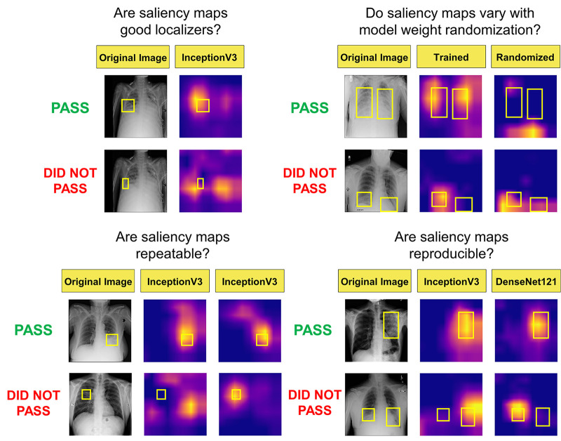
Considering the combination of the above-mentioned trustworthiness criteria provides a blueprint for us to assess a saliency map’s localization capabilities (localization utility), sensitivity to trained model weights (vs randomized weights), and accuracy with respect to models trained with the same architectures (repeatability) and different architectures (reproducibility). Figure 1 summarizes the questions addressed in this work.

Figure 1:

Visualization of the different questions addressed in this work. Note that the top rows of images and saliency maps demonstrate ideal (and less commonly observed) high-performing examples (“pass”), while the bottom rows of images demonstrate realistic (and more commonly observed) poor-performing examples (“did not pass”). First, we examined whether saliency maps are good localizers in regard to the extent of the maps’ overlap with pixel-level segmentations or ground truth bounding boxes. Next, we evaluated whether saliency maps were affected when trained model weights were randomized, indicating how closely the maps reflect model training. Then we generated saliency maps from separately trained InceptionV3 models to assess their repeatability. Finally, we assessed the reproducibility by calculating the similarity of saliency maps generated from different models (InceptionV3 and DenseNet-121) trained on the same data.

Data Preparation

Institutional review board approval was not required for this retrospective study; the chest radiographs used in this study were obtained from publicly available datasets on Kaggle (12,14).

The SIIM-ACR Pneumothorax Segmentation dataset consists of 10 675 images, split into 81% training, 9% validation, and 10% testing. The training set comprised 8646 images with 1931 patients with pneumothorax, the validation set had 961 images with 202 patients with pneumothorax, and the test set had 1068 images with 246 patients with pneumothorax.

The RSNA Pneumonia Detection Challenge dataset consists of 14 863 images, which was split in a similar fashion as described above for the pneumothorax dataset. The final training set comprised 12 039 images with 4870 patients with pneumonia, the validation set had 1338 images with 541 patients with pneumonia, and the test set had 1486 images with 601 patients with pneumonia.

Model Training

We trained InceptionV3 (16) and DenseNet-121 (17) models for all our experiments. The InceptionV3 network comprises several modules, allowing for more efficient computation and deeper networks through dimensionality reduction with stacked 1 × 1 convolutions. The DenseNet-121 network comprises four blocks with six, 12, 24, and 16 layers each, which extract features to be sent to a classification module. These image classification model backbones were modified by replacing the final layer to perform binary classification. The models were loaded with pretrained weights on ImageNet, which were then fine-tuned during training. Both InceptionV3 and DenseNet-121 models are trained using binary cross-entropy loss:

Further details about model training are in Appendix E1(supplement).

Saliency Methods and Evaluation Criteria

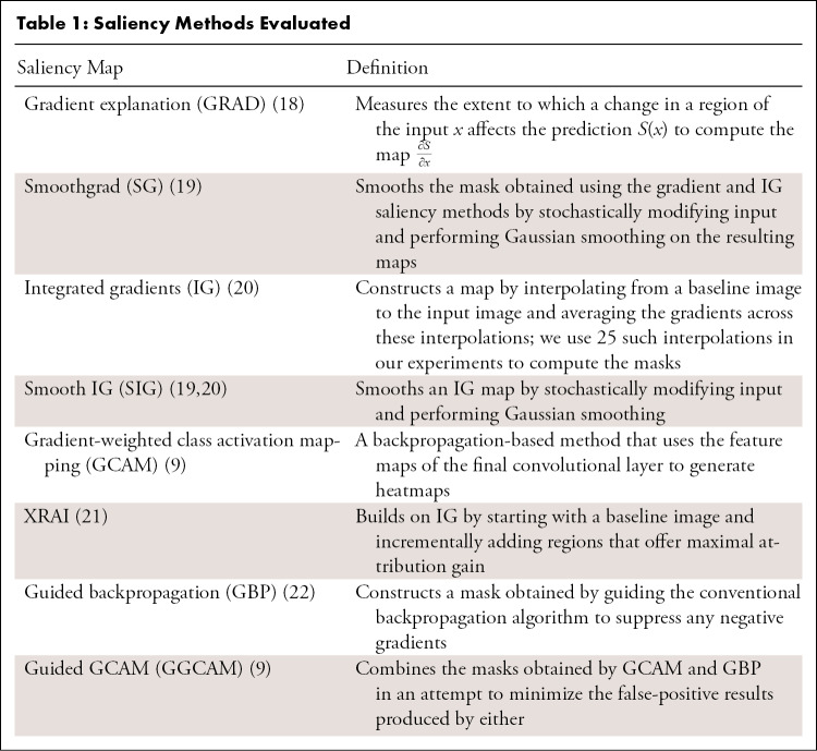
For model interpretability, we evaluated the following saliency methods: gradient explanation (GRAD) (18), Smoothgrad (SG) (19), integrated gradients (IG) (20), smooth IG (SIG) (19,20), gradient-weighted class activation mapping (GCAM) (9), XRAI (21), guided backpropagation (GBP) (22), and guided GCAM (GGCAM) (9). All methods are summarized and defined in Table 1. We compared the performance of these saliency maps against the following baselines: (a) for localization utility, a low baseline defined by a single “average” mask of all ground truth segmentations or bounding boxes in the training and validation datasets (AVG) and a high baseline determined by the area under the precision recall curve (AUPRC [23]) of segmentation (U-Net) and detection networks (RetinaNet); (b) in model weight randomization, the average value of the structural similarity index measure (SSIM) of 50 randomly chosen pairs of saliency maps pertaining to the fully trained model (randomization baseline); and (c) in repeatability and reproducibility, a low baseline of an SSIM of 0.5 and a high baseline determined by the SSIM of U-Net and RetinaNet. Note that a low baseline of 0.5 for SSIM was chosen because SSIM ranges from 0 (for lack of any structural similarity) to 1 (for identical structural similarity), and 0.5 marks the midpoint for whether the SSIM is more structurally similar or dissimilar (24). SSIM is a metric used for evaluating image similarity computed as a weighted combination of the comparison measurements of luminance, contrast, and structure. An SSIM of 1 is achieved when comparing identical sets of data, whereas an SSIM of 0 indicates no structural similarity. Note that throughout this section, a “pass” is denoted if the saliency method had a higher performance than the respective baseline, while a “did not pass” is denoted if the saliency method had a lower performance than the respective baseline (described further in Tables 2 and 3). If “uncertain” is denoted, this indicates that there was no significant difference between the performance of the saliency map and the corresponding baseline.

Table 1:

Saliency Methods Evaluated

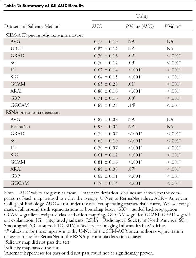
Table 2:

Summary of All AUC Results

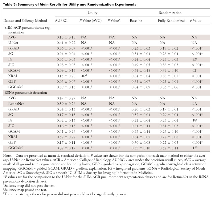
Table 3:

Summary of Main Results for Utility and Randomization Experiments

Although saliency maps were not originally intended for either segmentation or detection, they have been used this way in clinical research to identify areas of abnormality from trained neural networks (6–8). Using saliency maps in this manner can cause potential problems when this type of research is applied to clinical practice. Therefore, we chose to evaluate saliency maps using pixel-based metrics to show the discrepancies with using them in such a manner and provide objective measures as to why using saliency maps in place of segmentation or detection may not be ideal in clinical scenarios. We choose AUPRC as the metric to capture localizability of saliency maps, as the relatively small size of the ground truth segmentation masks and bounding boxes would benefit from an approach that would account for the class imbalance. Precision recall curves better serve to be more informative about the performance of an algorithm, particularly for unbalanced datasets with few positive pixels relative to the number of negative pixels. In the context of findings on medical images, the area under the receiver operating characteristic curve (AUC) can be skewed by the presence of a large number of true-negative findings (25).

Precision is defined as the ratio of true-positive findings to predicted positive findings (true-positive findings + false-positive findings), while recall is defined as the ratio of true-positive findings to ground truth positive findings (true-positive findings + false-negative findings). Since neither of these account for the number of true-negative findings, they make ideal candidates for our analysis. To capture the intersection between the saliency maps and segmentation masks or bounding boxes, we considered the pixels inside the segmentations or boxes to be positive labels and those outside to be negative. Each pixel of the saliency map is thus treated as an output from a binary classifier. An ideal saliency map, from the perspective of utility, would have perfect recall (finding all regions of interest) without labeling any pixels outside the regions of interest as positive (perfect precision).

To investigate the sensitivity of saliency methods under changes to model parameters and to identify potential correlation of particular layers to changes in the maps, we employed cascading randomization on the InceptionV3 model (6). In cascading randomization, we successively randomized the weights of the model, beginning from the top layer to the bottom, effectively erasing the learned weights in a gradual fashion. We used the SSIM to assess the change of the original saliency map with the saliency maps generated from the model after each randomization step (26).

Additionally, to test if the saliency methods produce similar maps with a different set of trained weights and whether they were architecture agnostic (assuming that models with different trained weights or architectures have similar classification performance), we conducted repeatability tests on the saliency methods by comparing maps from (a) different randomly initialized instances of models with the same architecture trained to convergence (intra-architecture repeatability) and (b) models with different architectures each trained to convergence (interarchitecture reproducibility) using SSIM between saliency maps produced from each model. Although there was no constraint that indicated that interpretations should be the same across models, an ideal trait of a saliency map would be to have some degree of robustness across models with different trained weights or architectures.

Training details of the models, corresponding baselines (U-Net for segmentation, RetinaNet for detection), and additional description of the utility metric (AUPRC) are provided in Appendix E1(supplement).

Statistical Analysis

Statistical analyses were performed in RStudio version 1.2.5033 using R 3.6 and the lmer (lme4, version 1–1-25), lmerTest (version 3.1–3), ggplot2 (version 3.3.2), and multComp (version 1.4–14) packages. A linear mixed-effects model was used to evaluate trustworthiness of the eight saliency map methods using a two-sided test with α level set at .05 for statistical significance. Tukey honestly significant difference test was used for post hoc analysis. For our statistical analysis, we assessed four main questions. First, we determined if there were differences in the utilities between saliency map methods derived from the trained classification models compared with the utility of the localization networks (U-Net for segmentation and RetinaNet for detection). Second, we determined if there were differences in the performances between the saliency maps and the average mask (ie, average of segmentations or bounding boxes from the training and validation sets) in terms of the utility of the map. Third, we assessed if saliency maps degraded to the level of the randomization baseline when the model weights of the trained model were randomized. Last, we assessed if there were any differences in the repeatability and/or reproducibility of each of the saliency map methods compared with the performance of the low baseline (ie, SSIM = 0.5) or the localization networks (U-Net for segmentation and RetinaNet for detection).

Results

Localization Utility

Segmentation utility.— We evaluated the localization utility of each saliency method by quantifying their intersection with ground truth pixel-level segmentations available from the pneumothorax dataset. We compared the saliency methods with the average of the segmentations across the training and validation sets (low baseline), as well as a U-Net (7) trained to learn these segmentations directly (high baseline). Note that the average mask baseline was introduced as a criterion that should be easy for any saliency method to outperform. While the saliency maps were generated independently for each specific image, the average mask was a single map that is applied across all images in the test set and hence is a minimum bar for evaluation of this task. We defined the average mask as low baseline as a threshold for the saliency maps to outperform.

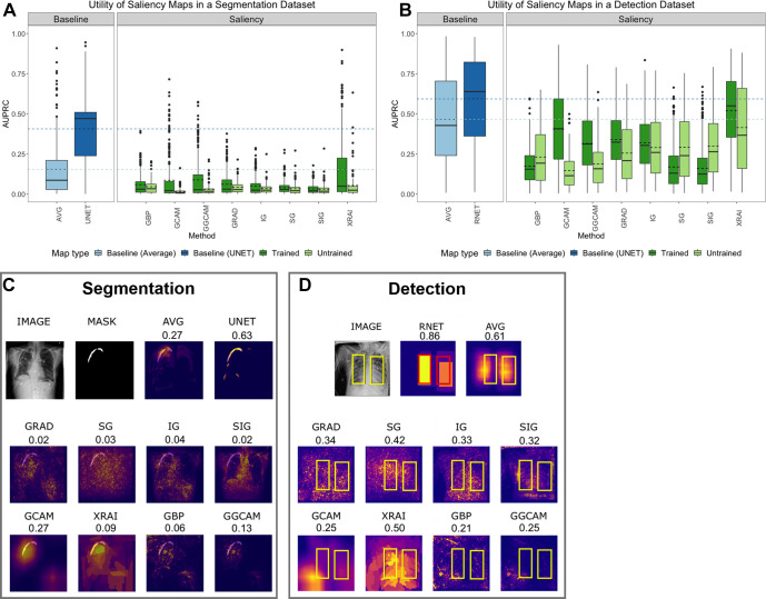
Saliency maps generated from InceptionV3 demonstrated higher utility than those generated from DenseNet-121 and are displayed in Figure 2A. For individual saliency maps on InceptionV3, the highest performing method was XRAI (AUPRC, 0.15 ± 0.20), while the lowest performing method was SIG (AUPRC, 0.03 ± 0.03). It is also interesting to note that using the average of all masks across the pneumothorax training and validation datasets (AVG) performed as well or higher than most of the saliency methods (AUPRC, 0.15 ± 0.18), showing a strong limitation in the saliency maps’ validity. Specifically, XRAI performed higher than the average map (P = .02), while the other saliency methods had lower AUPRCs (P < .001 for all). Additionally, the U-Net trained on a segmentation task achieved the highest utility (AUPRC, 0.41 ± 0.22), and the utility of all maps was lower than the U-Net (P < 0.001 for all).

Figure 2:

(A) Test set segmentation AUPRC scores for SIIM-ACR Pneumothorax Segmentation dataset and (B) test set bounding box detection AUPRC scores for RSNA Pneumonia Detection Challenge dataset. Each box plot represents the distribution of scores across the test datasets for each saliency map, with a solid line denoting the median and a dashed line denoting the mean. Results are compared with a low baseline using the average segmentation or bounding box of the training and validation sets (light blue) and high baseline using U-Net or RetinaNet (dark blue). (C) Example saliency maps on SIIM-ACR pneumothorax dataset with corresponding AUPRC scores and (D) on RSNA pneumonia dataset with corresponding utility scores. “AVG” refers to using the average of all ground-truth masks (for pneumothorax) or bounding boxes (for pneumonia) across the training and validation datasets; “UNET” refers to using the U-Net trained on a segmentation task for localization of pneumothorax; “RNET” refers to using RetinaNet to generate bounding boxes for localizing pneumonia with bounding boxes. ACR = American College of Radiology, AUPRC = area under the precision-recall curve, GBP = guided backpropagation, GCAM = gradient-weighted class activation mapping, GGCAM = guided GCAM, GRAD = gradient explanation, IG = integrated gradients, RSNA = Radiological Society of North America, SG = Smoothgrad, SIG = smooth IG, SIIM = Society for Imaging Informatics in Medicine.

The utility of the saliency maps generated using the trained models was higher than the random models for SG (AUPRC, trained: 0.04 ± 0.04 vs random: 0.03 ± 0.04; P = .004), GCAM (trained: 0.09 ± 0.14 vs random: 0.02 ± 0.02; P < .001), XRAI (trained: 0.15 ± 0.20 vs random: 0.05 ± 0.09; P < .001), and GGCAM (trained: 0.09 ± 0.13 vs random: 0.03 ± 0.04; P = .002), but not for GBP, GRAD, IG, and SIG.

Tests comparing the utilities in terms of the AUC were also performed and are summarized in Table 2. When compared with AVG, there were only two minor differences from AUPRC: (a) GBP was uncertain for AUC (P = .08), while it did not pass for AUPRC (P < .001), and (b) GGCAM was uncertain for AUC (P = .14), while it did not pass for AUPRC (P < .001). When compared with U-NET, there were no major differences among the eight different mapping methods.

Detection utility.— We evaluated the detection utility of each saliency method using the ground truth bounding boxes from the pneumonia detection dataset. Figure E1 (supplement) shows visualizations of saliency maps generated from InceptionV3 on the pneumonia detection dataset. We compared the saliency methods with the average of the bounding boxes across the training and validation sets (low baseline), as well as a RetinaNet (27) trained to learn these bounding boxes directly (high baseline).

Results for the test set are shown in Figure 2B. The highest-performing saliency method was XRAI (AUPRC, 0.52 ± 0.22), while the lowest performing method was SIG (AUPRC, 0.16 ± 0.13). It is interesting to note that using the average of all bounding boxes across the pneumonia training and validation datasets (AVG) performed higher than all the methods (AUPRC, 0.47 ± 0.27) except for XRAI, which had a higher performance (P < .001). RetinaNet trained to generate bounding boxes achieved a higher performance than all the saliency methods (AUPRC, 0.59 ± 0.26; P < .001 for all comparisons).

The utility of saliency maps generated using the trained models was higher than the utility of the random models for GRAD (trained: 0.34 ± 0.16 vs random: 0.26 ± 0.17; P < .001), GCAM (trained: 0.41 ± 0.23 vs random: 0.15 ± 0.12; P < .001), XRAI (trained: 0.52 ± 0.22 vs random: 0.41 ± 0.26; P < .001), and GGCAM (trained: 0.32 ± 0.17 vs random: 0.19 ± 0.15; P < .001). The random model had higher performance SG (trained: 0.17 ± 0.13 vs random: 0.29 ± 0.20; P < .001) and SIG (trained: 0.16 ± 0.13 vs random: 0.30 ± 0.19; P < .001), and there were no statistical differences for IG (trained: 0.32 ± 0.16 vs random: 0.29 ± 0.18; P = .06).

Tests comparing the utilities in terms of AUC were also performed and are summarized in Table 2. There was only one minor difference from AUPRC: When compared with AVG, XRAI was uncertain for AUC (P = .87), while it passed for AUPRC (P < .001).

Sensitivity to Trained versus Random Model Weights

Saliency maps should be sensitive to model weights to be meaningful. Specifically, a saliency map generated from a trained model should differ from a randomly initialized model, which has no knowledge of the task.

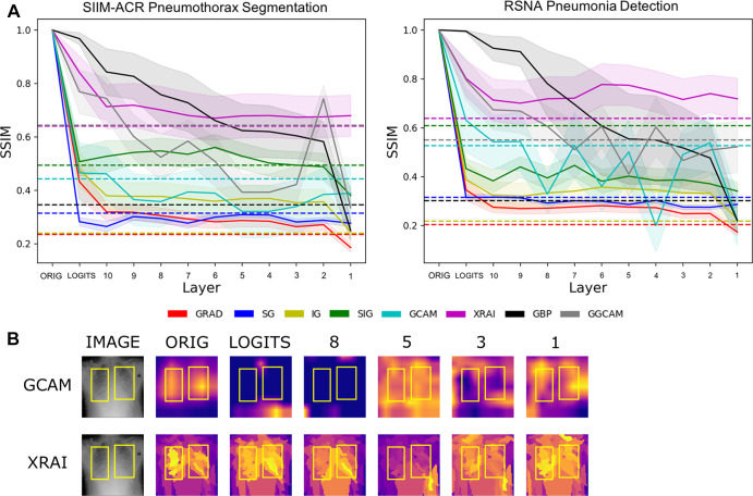
Figure 3A shows the progressive degradation of saliency maps, and Figure 3B shows an example image of saliency map degradation from cascading randomization. Figure E2 (supplement) shows additional examples. Table 3 shows the mean SSIM scores of saliency maps for fully randomized models (after cascading randomization has reached the bottommost layer), as well as the corresponding randomization baselines, defined below.

Figure 3:

(A) Structural similarity index measures (SSIMs) under cascading randomization of modules on InceptionV3 for the SIIM-ACR Pneumothorax Segmentation dataset and RSNA Pneumonia Detection Challenge dataset. Note that the colored dotted lines correspond to the randomization baseline for each saliency map, which were generated by the average SSIMs of 50 randomly chosen pairs of saliency maps pertaining to the fully trained model; a saliency model successfully reaches degradation if it goes below its corresponding randomization baseline. (B) Example image from RSNA pneumonia detection dataset to visualize saliency map degradation from cascading randomization. “Logits” refers to the logit layer (final layer) of the InceptionV3 model, and layer blocks 1 through 10 refer to blocks mixed 1 through mixed 10 in the original InceptionV3 architecture. ACR = American College of Radiology, GBP = guided backpropagation, GCAM = gradient-weighted class activation mapping, GGCAM = guided GCAM, GRAD = gradient explanation, IG = integrated gradients, Orig = original, RSNA = Radiological Society of North America, SG = Smoothgrad, SIG = smooth IG, SIIM = Society for Imaging Informatics in Medicine.

A saliency map reached degradation and was classified as a pass when the average SSIM was not significantly different or below the randomization baseline. For both pneumothorax and pneumonia datasets, we observed that XRAI did not reach the randomization baseline when cascading randomization had reached the bottommost layer (ie, full randomization), showing invariance to the trained model parameters. The saliency maps that fell below this randomization baseline on both datasets when the model was fully randomized include GCAM, GBP, GRAD, SG, and SIG, showing a dependency on the model weights, which is desired.

Repeatability and Reproducibility

To investigate intra-architecture repeatability and interarchitecture reproducibility, the SSIMs of saliency maps produced from (a) models sharing the same architecture but different random initializations and (b) models with different architecture classes were analyzed. In both cases, the models were trained to convergence. For comparison, we used a low baseline of SSIM = 0.5 (since SSIM = 0.5 marks the midpoint for whether the SSIM is more structurally similar or dissimilar) and a high baseline of repeatability and reproducibility of separately trained U-Nets (for the pneumothorax dataset) and RetinaNets (for the pneumonia dataset).

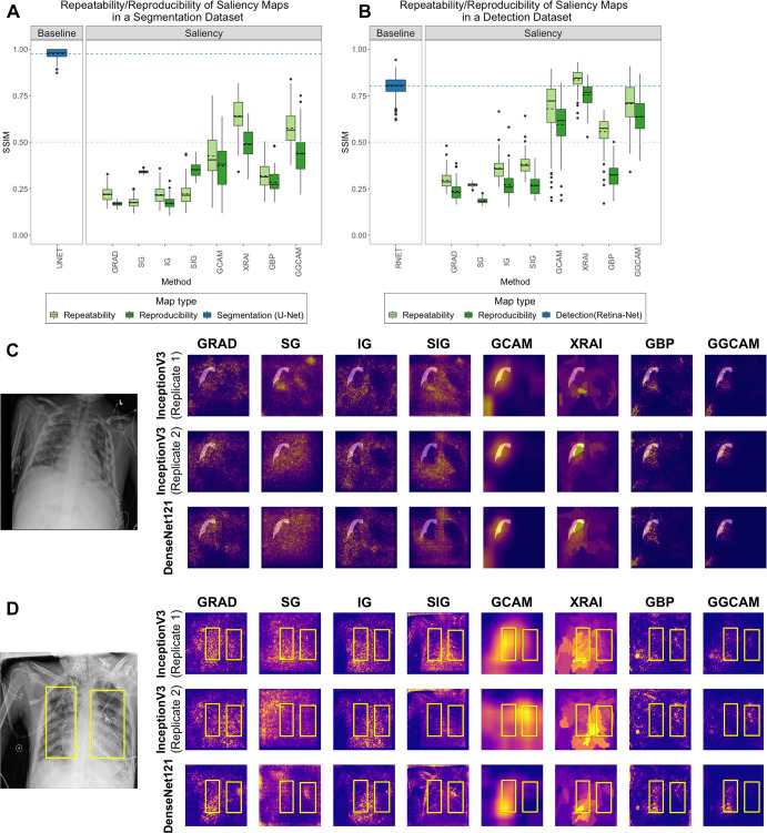
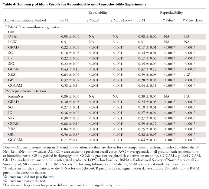
We examined the repeatability of saliency methods from two separately trained InceptionV3 models and the reproducibility of saliency methods from trained InceptionV3 and DenseNet-121 models. Figures 4A and 4B summarize the results for the pneumothorax and pneumonia datasets, respectively. In the pneumothorax dataset, the baseline U-Net achieved an SSIM of 0.98 ± 0.02, which was higher than the SSIM values from any of the other saliency maps (P < .001 for all comparisons). The low baseline of SSIM of 0.5 was higher than the SSIM of any of the other saliency maps except for the repeatability of XRAI and GGCAM. Among the saliency maps, XRAI had the highest repeatability (SSIM, 0.64 ± 0.09), while SG has the lowest repeatability (SSIM, 0.18 ± 0.03). For reproducibility, XRAI had the highest SSIM (0.49 ± 0.08), while GRAD had the lowest SSIM (0.17 ± 0.01).

Figure 4:

Comparison of repeatability and reproducibility scores for all saliency methods for (A) SIIM-ACR Pneumothorax Segmentation dataset and (B) RSNA Pneumonia Detection Challenge dataset. Each box plot represents the distribution of scores across the test datasets for each saliency map, with a solid line denoting the median and a dashed line denoting the mean. Results are compared with a low baseline of SSIM = 0.5 (light blue dashed line) and high baseline using U-Net or RetinaNet (dark blue box plot and dashed line). Two examples of repeatability (InceptionV3 replicates 1 and 2) and reproducibility (InceptionV3 and DenseNet-121) for the (C) SIIM-ACR pneumothorax dataset with transparent segmentations and (D) RSNA pneumonia dataset with yellow bounding boxes. The first two rows of (C) and (D) are saliency maps generated from two separately trained InceptionV3 models (replicates 1 and 2) to demonstrate repeatability, and the last row are saliency maps generated by DenseNet-121 to demonstrate reproducibility. GBP = guided backpropagation, GCAM = gradient-weighted class activation mapping, GGCAM = guided GCAM, GRAD = gradient explanation, IG = integrated gradients, RSNA = Radiological Society of North America, SG = Smoothgrad, SIG = smooth IG, SIIM = Society for Imaging Informatics in Medicine, SSIM = structural similarity index measure.

In the pneumonia dataset, the baseline RetinaNet achieved an SSIM of 0.80 ± 0.05, which was only exceeded by XRAI’s repeatability score (P < .001). The low baseline of 0.5 SSIM was greater than the performance of all saliency maps except the repeatability and reproducibility of GCAM, GGCAM, and XRAI and the repeatability of GBP. Among the saliency maps, XRAI had the highest repeatability (SSIM, 0.84 ± 0.06), while SG had the lowest (SSIM, 0.27 ± 0.01). For reproducibility, XRAI had the highest SSIM (0.75 ± 0.06), while SG had the lowest SSIM (0.18 ± 0.01). Repeatability was higher than reproducibility for all methods (P < .001). Overall, XRAI had the highest repeatability and reproducibility across different datasets. Figure E3 (supplement) shows additional examples for repeatability and reproducibility, and Table 4 demonstrates the overall results for each saliency map across all tests. A pass in Table 4 is denoted if the saliency method had a higher performance than the respective baseline, while a did not pass is denoted if the saliency method performed lower than the respective baseline (described further in Table 4).

Table 4:

Summary of Main Results for Repeatability and Reproducibility Experiments

Discussion

In this study, we evaluated the performance and robustness of several popular saliency maps on medical images. By considering saliency map utility with respect to localization, sensitivity to model weight randomization, repeatability, and reproducibility, we demonstrated that none of the saliency maps met all tested criteria, and their credibility should be critically evaluated prior to integration into medical imaging pipelines. This is particularly important because many recent deep learning–based clinical studies rely on saliency maps for interpretability of deep learning models without noting and critically evaluating their inherent limitations. A recent empirical study found that ophthalmologists and optometrists rated GBP highly as an explainability method, despite the limitations we note in this study (28). From Table 3 and Table 4, none of the maps pass all four defined trustworthiness criteria, and in fact, most of them perform lower than their corresponding baselines. For their high baseline methods, the utility, repeatability, and reproducibility tasks use networks that train specifically as localizers (ie, U-Net and RetinaNet). With the exception of XRAI on repeatability in the pneumonia dataset, all the saliency maps had a lower performance than U-Net and RetinaNet. This highlights a severe limitation in the saliency maps as a whole and shows that using models trained directly on localization tasks (such as U-Net and RetinaNet) greatly improves the results. To inform future saliency map development, we can consider some aspects of the better-performing maps. In regard to utility, XRAI had the highest performance (in terms of AUPRC) for both segmentation and detection tasks. For each test image in the dataset, XRAI segments the image into small regions, iteratively evaluates the relevance of each region to the model prediction, and aggregates the smaller regions into a larger region based on the relevance scores. The iterative evaluation of small patches within the image likely gives XRAI an advantage over other methods, as it results in maps with better fine-grained localization catering to the adjacent spatial neighborhoods, thus achieving a higher recall and precision than the other methods. In regard to cascading randomization across different layers of the InceptionV3 model, GCAM passed the randomization test, demonstrating a dependence of the map on the learned parameters. GCAM forward propagates test images through the model to obtain a prediction, then backpropagates the gradient of the predicted class to the desired convolutional feature map (29). As a result, there is a high sensitivity to the value of the weights in the model. Finally, for both datasets, XRAI demonstrated the highest repeatability score between two separately trained models with the same architecture and also the highest reproducibility between two separately trained models with different architectures. XRAI’s aggregation of smaller regions into larger regions likely reduces the influence of variability across trained models with similar architectures. Thus, the overall model weight distribution should remain the same in a specific area for a particular image even if the models are separately trained. However, these properties have not yet been extensively studied because XRAI is a fairly new saliency method. Additional insights for the results of each task are provided in Appendix E1 (supplement).

Depending on the desired outcome of interpretability, there are alternative techniques besides saliency methods that can be employed. One approach would be to train CNNs that output traditional handcrafted features (such as shape and texture) as intermediates (30). This approach would provide some interpretability but is limited by the utility and reliability of the handcrafted features. Another approach may also be to use interpretable models in the first place. Rudin argues that instead of creating methods to interpret black box models trained for high-stakes decision-making, we should instead put our focus on designing models that are inherently interpretable (31). Rudin further argues that there is not necessarily a tradeoff between accuracy and interpretability, especially if the input data are well structured (ie, features are meaningful). Thus, the data from our study support the use of multiple avenues to improve model interpretation.

There were a few limitations to our study. First, we only evaluated saliency maps for two medical datasets, both consisting of chest radiographs. Future studies will examine more medical imaging datasets, including different image modalities and diseases. Additionally, we only performed tests on two CNN architectures, though these are commonly used networks in the literature for chest radiograph analysis (32,33). As a next step, we can examine the effect of other CNN architectures to determine if they result in saliency maps that are more repeatable and reproducible. Third, we focused only on the ability of saliency maps to localize pathologic features and thus the utility metrics were calculated using the regions of interest specifically (bounding boxes for pneumonia and segmentation maps for pneumothorax). These regions of interest may not include other image features that can contribute to classification algorithm performance, known as hidden stratification. For example, a chest tube in an image would imply the presence of a pneumothorax, but much of the chest tube may not be in the region of interest (34). More global features could also contribute to classification. For example, low lung volumes and portable radiograph technique may suggest that the patient is hospitalized, which could be associated with likelihood of pneumonia. These features would also not be covered in the regions of interest. Future work can evaluate the utility of saliency maps to localize these other features. We could also investigate incorporating saliency maps as a part of neural network training and evaluate if this type of approach results in maps that have higher utility than maps that are generated after model training (35).

The eight considered saliency maps studied are quantitatively shown to underperform in several key criteria including localization utility, parameter sensitivity, repeatability, and reproducibility. This carries notable clinical importance, as saliency methods are widely used in medical studies for model interpretation and localization. We advocate that the inclusion of these methods into medical imaging projects be scrutinized and only take place with the knowledge of their shortcomings.

References

- 1. Chang K , Beers AL , Brink L , et al . Multi-institutional assessment and crowdsourcing evaluation of deep learning for automated classification of breast density . J Am Coll Radiol 2020. ; 17 ( 12 ): 1653 – 1662 . [DOI] [PMC free article] [PubMed] [Google Scholar]
- 2. Li MD , Chang K , Bearce B , et al . Siamese neural networks for continuous disease severity evaluation and change detection in medical imaging . NPJ Digit Med 2020. ; 3 48 . [DOI] [PMC free article] [PubMed] [Google Scholar]
- 3. Li MD , Arun NT , Gidwani M , et al . Automated assessment and tracking of COVID-19 pulmonary disease severity on chest radiographs using convolutional siamese neural networks . Radiol Artif Intell 2020. ; 2 ( 4 ): e200079 . [DOI] [PMC free article] [PubMed] [Google Scholar]
- 4. Saba T , Khan MA , Rehman A , Marie-Sainte SL . Region extraction and classification of skin cancer: A heterogeneous framework of deep CNN features fusion and reduction . J Med Syst 2019. ; 43 ( 9 ): 289 . [DOI] [PubMed] [Google Scholar]
- 5. Jeyaraj PR , Samuel Nadar ER . Computer-assisted medical image classification for early diagnosis of oral cancer employing deep learning algorithm . J Cancer Res Clin Oncol 2019. ; 145 ( 4 ): 829 – 837 . [DOI] [PMC free article] [PubMed] [Google Scholar]
- 6. Rajpurkar P , Irvin J , Zhu K , et al . CheXNet: Radiologist-Level Pneumonia Detection on Chest X-Rays with Deep Learning . arXiv:1711.05225 [preprint] https://arxiv.org/abs/1711.05225. Posted November 14, 2017. Accessed August 2019 .
- 7. Bien N , Rajpurkar P , Ball RL , et al . Deep-learning-assisted diagnosis for knee magnetic resonance imaging: Development and retrospective validation of MRNet . PLoS Med 2018. ; 15 ( 11 ): e1002699 . [DOI] [PMC free article] [PubMed] [Google Scholar]
- 8. Mitani A , Huang A , Venugopalan S , et al . Detection of anaemia from retinal fundus images via deep learning . Nat Biomed Eng 2020. ; 4 ( 1 ): 18 – 27 . [DOI] [PubMed] [Google Scholar]
- 9. Eitel F , Ritter K , Alzheimer’s Disease Neuroimaging Initiative (ADNI) , et al . Testing the robustness of attribution methods for convolutional neural networks in MRI-based Alzheimer’s disease classification . Interpretability of Machine Intelligence in Medical Image Computing and Multimodal Learning for Clinical Decision Support . Cham, Switzerland: : Springer; , 2019. ; 3 – 11 . [Google Scholar]
- 10.Young K, Booth G, Simpson B, Dutton R, Shrapnel S. Deep neural network or dermatologist? In: Suzuki K, Reyes M, Syeda-Mahmood T, et al., eds.interpretability of machine intelligence in medical image computing and multimodal learning for clinical decision support. ML-CDS 2019, IMIMIC 2019. Lecture Notes in Computer Science, vol 11797.Cham, Switzerland:Springer,2019;48–55. [Google Scholar]
- 11. Sayres R , Taly A , Rahimy E , et al . Using a deep learning algorithm and integrated gradients explanation to assist grading for diabetic retinopathy . Ophthalmology 2019. ; 126 ( 4 ): 552 – 564 . [DOI] [PubMed] [Google Scholar]
- 12. SIIM-ACR Pneumothorax Segmentation . Kaggle . https://www.kaggle.com/c/siim-acr-pneumothorax-segmentation. Published 2019. Accessed September 2019 .
- 13. Tolkachev A , Sirazitdinov I , Kholiavchenko M , Mustafaev T , Ibragimov B . Deep learning for diagnosis and segmentation of pneumothorax: the results on the kaggle competition and validation against radiologists . IEEE J Biomed Health Inform 2021. ; 25 ( 5 ): 1660 – 1672 . [DOI] [PubMed] [Google Scholar]
- 14. RSNA Pneumonia Detection , https://www.kaggle.com/c/rsna-pneumonia-detection-challenge. Published 2018. Accessed August 2019 .
- 15. Shih G , Wu CC , Halabi SS , et al . Augmenting the National Institutes of Health chest radiograph dataset with expert annotations of possible pneumonia . Radiol Artif Intell 2019. ; 1 ( 1 ): e180041 . [DOI] [PMC free article] [PubMed] [Google Scholar]
- 16. InceptionV3 . GitHub . https://github.com/keras-team/keras-applications/blob/master/keras_applications/inception_v3.py. Published 2019. Accessed August 2019 .
- 17. DenseNet121. GitHub . https://github.com/keras-team/keras-applications/blob/master/keras_applications/densenet.py. Published 2018. Accessed August 2019 .
- 18. Simonyan K , Vedaldi A , Zisserman A . Deep inside convolutional networks: visualising image classification models and saliency maps . arXiv:1312.6034 [preprint] https://arxiv.org/abs/1312.6034. Posted December 20, 2013. Accessed July 2019 .
- 19. Smilkov D , Thorat N , Kim B , Viégas F , Wattenberg M . SmoothGrad: removing noise by adding noise . arXiv:1706.03825 [preprint]https://arxiv.org/abs/1706.03825. Posted June 12, 2017. Accessed July 2019 .
- 20.Sundararajan M, Taly A, Yan Q. Axiomatic attribution for deep networks. Proceedings of the 34th International Conference on Machine Learning-Volume 70,2017;3319–3328.JMLR.org. [Google Scholar]
- 21.Adebayo J, Gilmer J, Muelly M, Goodfellow I, Hardt M, Kim B. Sanity checks for saliency maps. Adv Neural Inf Process Syst 2018; vol. 25:9505“9515. [Google Scholar]
- 22. Springenberg JT , Dosovitskiy A , Brox T , Riedmiller M . Striving for Simplicity: The All Convolutional Net . arXiv:1412.6806 [preprint]https://arxiv.org/abs/1412.6806. Posted December 21, 2014. Accessed September 2019 .
- 23. Boyd K , Eng KH , Page CD . Area under the precision-recall curve: point estimates and confidence intervals . Joint European Conference on Machine Learning and Knowledge Discovery in Databases . Berlin: : Springer; , 2013. ; 451 – 466 . [Google Scholar]
- 24. Renieblas GP , Nogués AT , González AM , Gómez-Leon N , Del Castillo EG . Structural similarity index family for image quality assessment in radiological images . J Med Imaging (Bellingham) 2017. ; 4 ( 3 ): 035501 . [DOI] [PMC free article] [PubMed] [Google Scholar]
- 25. Ozenne B , Subtil F , Maucort-Boulch D . The precision--recall curve overcame the optimism of the receiver operating characteristic curve in rare diseases . J Clin Epidemiol 2015. ; 68 ( 8 ): 855 – 859 . [DOI] [PubMed] [Google Scholar]
- 26.Zar JH. Spearman rank correlation. In: Encyclopedia of Biostatistics, Vol 7.Wiley Online Library,2005. [Google Scholar]
- 27. Lin TY , Goyal P , Girshick R , He K , Dollár P . Focal loss for dense object detection . Proceedings of the IEEE International Conference on Computer Vision, Conference Location, Conference date . Piscataway, NJ : IEEE; , 2017. ; 2980 – 2988 . [Google Scholar]
- 28. Singh A , Balaji JJ , Jayakumar V , Rasheed MA , Raman R , Lakshminarayanan V . Quantitative and Qualitative Evaluation of Explainable Deep Learning Methods for Ophthalmic Diagnosis . arXiv:2009.12648 [preprint] https://arxiv.org/abs/2009.12648. Posted September 26, 2020. Accessed October 2020 . [DOI] [PMC free article] [PubMed]
- 29. Selvaraju RR , Cogswell M , Das A , Vedantam R , Parikh D , Batra D . Grad-cam: Visual explanations from deep networks via gradient-based localization . Proceedings of the IEEE International Conference on Computer Vision, Conference Location, Conference date . Piscataway, NJ : IEEE; , 2017. ; 618 – 626 . [Google Scholar]
- 30. Lou B , Doken S , Zhuang T , et al . An image-based deep learning framework for individualizing radiotherapy dose . Lancet Digit Health 2019. ; 1 ( 3 ): e136 – e147 . [DOI] [PMC free article] [PubMed] [Google Scholar]
- 31. Rudin C . Stop explaining black box machine learning models for high stakes decisions and use interpretable models instead . Nat Mach Intell 2019. ; 1 ( 5 ): 206 – 215 . [DOI] [PMC free article] [PubMed] [Google Scholar]
- 32. Narin A , Kaya C , Pamuk Z . Automatic detection of coronavirus disease (COVID-19) using X-ray images and deep convolutional neural networks . arXiv:2003.10849 [preprint] https://arxiv.org/abs/2003.10849. Posted March 24, 2020. Accessed April 2020 . [DOI] [PMC free article] [PubMed]
- 33. Rajpurkar P , Irvin J , Ball RL , et al . Deep learning for chest radiograph diagnosis: A retrospective comparison of the CheXNeXt algorithm to practicing radiologists . PLoS Med 2018. ; 15 ( 11 ): e1002686 . [DOI] [PMC free article] [PubMed] [Google Scholar]
- 34. Oakden-Rayner L , Dunnmon J , Carneiro GR . Hidden stratification causes clinically meaningful failures in machine learning for medical imaging . Proceedings of the ACM Conference on Health, Inference, and Learning , 2020. . [DOI] [PMC free article] [PubMed] [Google Scholar]
- 35. Alzantot M , Widdicombe A , Julier S , Srivastava M . NeuroMask: Explaining Predictions of Deep Neural Networks through Mask Learning . In: 2019 IEEE International Conference on Smart Computing (SMARTCOMP), Conference Location, Conference date . Piscataway, NJ : IEEE; , 2019. ; 81 – 86 . [Google Scholar]