Prospective Deployment of Artificial Intelligence in MRI: A Framework for Important Considerations, Challenges, and Recommendations for Best Practices

Abstract

Artificial intelligence algorithms based on principles of deep learning (DL) have made a large impact on the acquisition, reconstruction, and interpretation of MRI data. Despite the large number of retrospective studies using DL, there are fewer application of DL in the clinic on a routine basis. To address this large translational gap, we review the recent publications to determine three major use cases that DL can have in MRI, namely that of model-free image synthesis, model-based image reconstruction, and image or pixel-level classification. For each of these three areas, we provide a framework for important considerations that consists of appropriate model training paradigms, evaluation of model robustness, downstream clinical utility, opportunities for future advances, as well recommendations for best current practices. We draw inspirations for this framework from advances in computer vision in natural imaging as well as additional healthcare fields. We further emphasize the need for reproducibility of research studies through the sharing of datasets and software.

The advent and success of artificial intelligence and machine learning has energized the realm of medical imaging (1). Within MRI specifically, machine learning has impacted a multitude of pulse sequences and nearly all anatomies (2). Deep learning (DL), a subset of machine learning algorithms, has provided the spark necessary to fuel all these innovations (3). Most DL algorithms rely on the use of convolutional neural networks (CNN), which are non-linear feature extractors that can represent images and other signals at varying levels of hierarchical detail. By aggregating these multi-scale local and global patterns that exist within images, DL networks are capable of complex tasks, such as classifying the content of images and image transformations. Given the high-dimensional and multi-channel nature of MRI data along with the variations that can be introduced by different imaging hardware, artifacts, and patient anatomies, DL becomes a promising choice to interpret these highly heterogeneous images.

Currently, a handful of deep learning based solutions for MRI have been approved by the FDA under the software as a medical device designation for tasks such as image reconstruction, enhancement, segmentation, and classification (4). However, there is a dearth of studies comparing clinical utility of such DL models against the standard of care in large multi-center trials. Consequently, a large translational gap currently exists between technology development and technology deployment. To address the challenges in overcoming this translational chasm, in this review article, we provide a framework for important considerations for training and prospective deployment of DL models, beyond simply maximizing the accuracy DL models. For a comprehensive review of the fundamentals of DL, we refer to several different recent articles that provide an excellent description of the mechanisms and strategies commonly used in DL (5–7). In contrast, the goal of this review is to evaluate critically the current state of translational MRI DL research and to provide a high-level summary of the different opportunity areas and challenges for future use cases.

FRAMEWORK FOR CONSIDERATIONS AND OPPORTUNITIES:

The ability to apply DL to a variety of MRI techniques and anatomies is simultaneously a benefit and a challenge. Each technique and clinical use-case presents a unique need and optimization challenge, especially because the exact mechanisms underlying DL training and generalizability are known only through a limited set of empirical observations. We broadly categorize the different application areas of DL in MRI into model-free image synthesis, model-based reconstructions, and either pixel- or image-level classification tasks (Fig. 1). To mitigate prospective deployment challenges for these techniques, we will draw inspiration from computer vision for natural imaging and different medical imaging modalities to focus on the following areas important for translation considerations in this manuscript:

Figure 1:

An overview of the three generalized use-cases of deep learning (DL) and convolutional neural network (CNNs) in MRI. The first category relies on model-free contrast synthesis that synthesizes one image contrast or artifact status into another (a). A model-based reconstruction uses k-space data and embeds physics of Fourier encoding and data consistency into an iterative deep learning model to act as an additional regularizer (b). Images can be input into DL networks for assessment of imaging abnormalities (classification) or for segmentation specific tissues (c).

1. Training Paradigm: This notion entails the curation of the datasets for DL, CNN architectures, associated labels for training data, and loss functions that are used to solve a task of interest.

2. Robustness: After a model has been trained, how well can it be deployed in a useful clinical and research setting in light of variations in hardware, software, scan parameters, along with patient anatomies and populations?

3. Downstream Analysis: After training and evaluating robustness, how does the model inference affect the knowledge required to perform the clinical task at hand or to guide future treatment?

4. Opportunities: Considering the current status of the MRI and computer vision, are there specific short-term questions or challenges that can be addressed to provide efficient and robust training techniques and to maximize information available to enhance patient care?

5. Recommendations: What evidence can be provided to increase clinical confidence and drive adoption of the proposed techniques?

MODEL-FREE IMAGE SYNTHESIS:

Prior to DL, learning features or representations of images was based on developing hand-crafted image features such as gradient operators and filter banks (8). With the advent of DL-based models, more complex features can be automatically designed and extracted from images by building models that are more expressive to determine subtle variations in images. A variety of such DL tasks in MRI incorporate learning a mapping from an input image space to an output image space by learning the representation of the input data in a fully data-driven manner. Such end-to-end models do not utilize any external priors and do not consist of any external considerations or constraints in the intermediate and final outputs of the network. The benefit of such networks is directly related to the expressive power of CNNs and their ability to rapidly and simultaneously learn low-level image features (such as edges and shapes) as well as higher level features (such as the complex organization of multiple shapes and textures in images) (9).

These data-driven DL models have been used for many common image synthesis tasks, including image super-resolution, image denoising, artifact reduction, and contrast synthesis. Super-resolution is a long-studied task in computer vision that entails the recovery and estimation of high-resolution features from a low-resolution image (10). In MRI, super-resolution has recently been used to improve the resolution of a rapidly acquired low-resolution image by more than what is achievable through common interpolation algorithms (11, 12). Similarly, image denoising can model the distribution of image noise in order to remove the noise without blurring the true underlying image signal (13, 14). Analogous to denoising, DL can reduce the number of averages or directions required for accurate diffusion weighted imaging (15–17). Reducing MRI artifacts arising from motion, off-resonance, and Gibb’s ringing has also been addressed using a data-driven DL approach (18–20). DL has also allowed promising research to synthesize one medical imaging modality contrast to another; for example, DL algorithms can use MRI to estimate the appearance of a computed tomography (CT) image, which is beneficial for positron emission tomography attenuation correction (21, 22). Additionally, model-free contrast synthesis methods have estimated the appearance of contrast-enhanced brain MRI scans with a low-dose gadolinium input (23) and even a virtual contrast enhancement without any gadolinium input (24).

Training Paradigm:

Most image synthesis tasks employ fully supervised machine learning, which requires that every input image has a corresponding output image. However, acquiring a perfectly registered high-quality input and output image is not always feasible clinically, which limits CNN training to small datasets. Further, since this class of algorithms creates output images, there is a chance that additional image details not fundamentally present in the fully sampled imaging may be inadvertently created by the algorithm. Protecting against such image hallucinations is an active area of research (25). One possible technique to mitigate hallucination artifacts is through the use of residual images, which only generate sparse feature differences between an input and output image (26, 27). This allows the residual image to utilize the input image to learn a fundamental set of priors that constrain the output of images (Fig. 2). Generating only a residual output also implicitly forces network weights to be sparse and to automatically regularize themselves, similar to L2-regularization techniques (28, 29). Moreover, depending on the clinical use case and the amount of sparse residual content expected, an additional regularization term to limit the magnitude of the output of DL predictions may also mitigate hallucinations. In contrast to the problem of ‘false-positive’ hallucinations in images, there is also a risk of false-negatives by excluding true anatomical details. For examples, subtle features may accidentally be smoothed out if considered to be image noise. A common approach to mitigate this entails training with adequate representation of expected patient anatomies, which requires careful curation of training datasets that represent an approximate probability of expected anatomical variations.

Figure 2:

A residual-based CNN uses a low-quality input image (a low-resolution image in this case) and tries to create a sparse difference image between the low-resolution and high-resolution image. The sparsity of the model output limits the creation of hallucinated artifacts. A computation of the loss is performed by comparing the high-resolution ground truth to the sum of the low-resolution input and the sparse residual images.

Using model-free DL to solve ill-posed contrast-synthesis problems for MRI has the benefit of being entirely data-driven with minimal constraints placed on the models during optimization. However, without a defined model, it may be challenging to distinguish between true image signals and artifactual signals. In such an approach, incorporating the MRI encoding process and placing constraints on the conceivable outputs of a DL model may act as an additional regularization parameter to mitigate the impact of hallucinations or non-probable image signal.

An additional challenge with model-free approaches is the creation of the retrospective paired input-output datasets. For example, to create low-resolution images in super-resolution, high-resolution DICOM images are commonly Fourier transformed and cropped in k-space with a rectangular window or high-resolution images may be simply blurred with Gaussian kernels (12, 30). While these techniques may produce adequate results for the DL network, the downsampling process may not always fully reflect MRI encoding and does not take into effect complex-valued k-space domain data, ringing, or filtering. As a result, such approaches may have limited generalizability when applied to prospectively-acquired low-resolution datasets since the DL models have not learned an accurate representation of true low-resolution data. Thus, for model-free approaches, it is critical to develop an accurate processing pipeline to generate realistic high-quality and low-quality image pairs for supervised training.

Robustness

While training model-free algorithms, the concept of adversarial robustness, which is the ability of a trained network to withstand small perturbations in network inputs while maintaining accurate representations of input datasets, should be carefully considered (31). The need for adversarial robustness is highlighted in natural imaging when a correctly classified image is misclassified with high confidence following the addition of an imperceptible amount of noise. Sensitivity to adversarial noise can often be linked to out-of-distribution (OOD) datasets, wherein a network trained on a narrow distribution of input data cannot accurately represent data sampled from varying distributions (32). Adversarial robustness may be especially important in the context of DL MRI, where algorithms trained using images with a particular signal-to-noise ratio (SNR) may not generalize to images that have a lower SNR (33). Being robust to such adversarial examples implies lower susceptibility to OOD effects. For model-free systems, it is challenging to ensure data consistency between inputs and outputs, which further emphasizes the need for training robust networks through realistic data augmentations that minimize deleterious OOD effects. Common MRI artifacts such as motion or SNR corruption can be incorporated for data augmentation with the acquisition of k-space data, which can be intentionally degraded to build network robustness.

Downstream Analysis

The goal of medical imaging is not simply to image anatomy non-invasively, but rather, to use the images to assess any underlying abnormalities and organ status in either a qualitative or quantitative manner. However, most image generation algorithms conventionally use optimization metrics such as the structural similarity (SSIM), or L1 and L2 norms during the DL training process (34). While these metrics provide acceptable image quality, they do not always correspond to perceived image quality or diagnostic utility as assessed by human readers (35). This notion was recently highlighted during the evaluations of the fastMRI challenge, which provided a large-scale dataset of raw k-space data for developing DL-based undersampled 2D fast-spin-echo MRI reconstruction algorithms. There was considerable discordance between optimization of metrics such as SSIM and peak SNR (pSNR) that are used during image reconstruction, as compared to the opinions of expert radiologists in ascertaining image quality (36). In such scenarios, it becomes important not only to perform image quality optimization, but also to simultaneously evaluate the downstream utility and biases emanating from the reconstructed images. For example, it was shown that cardiac MRI super-resolution can be used to improve segmentation outcomes (37), knee MRI super-resolution can improve segmentation of cartilage as well as detection of small osteophytes (Fig. 3), and brain MRI super-resolution can improve depiction of cortical parcellation (Fig. 4) (38). Prior work has demonstrated that prospective super-resolution can simultaneously enhance image quality while maintaining quantitative accuracy of parametric T2 mapping (39) as well as diagnostic accuracy of rapid MRI scans (40). Consequently, while developing new loss functions for optimizing image quality remains an active research area, using model-free reconstruction approaches and evaluating their downstream clinical utility has the potential to provide an understanding of the overall utility and clinical applicability of the proposed techniques.

Figure 3:

Example images from a super-resolution technique used for threefold improving the resolution of sagittal double-echo steady-state knee MRI scans. Ground-truth original high-resolution (a,d), super-resolution images (b,e), and tricubic interpolated images (c,f) of axial (a-c) and coronal (d-f) reformations show the improvement that super-resolution brings about, especially in the case of subtle features such as cartilage (dashed arrow), thin collateral ligaments (dotted arrow), and effusion (solid arrow).

Figure 4:

Enlarged views of axial slices from ground-truth (a,b), down-sampled (b,c), spline up-sampled (e,f) and deep-learning super-resolution scans (g,h) in the primary visual cortex, with reconstructed gray matter-white matter surfaces and gray matter-cerebrospinal fluid (CSF) surfaces visualized as colored contours. All scans are 0.7mm isotropic resolution nominally, with the exception of the down-sampled scan that has a resolution of 1.0mm. Reconstructed surfaces displayed in (i,j) are overlaid on the ground-truth 0.7-mm isotropic T1-weighted images. Magenta arrowheads highlight locations where super-resolution images provided improved cortical surface estimates.

Opportunities

One of the largest opportunities for potential advances in clinically useful model-free DL algorithms is the development of quantitative metrics that estimate image quality as perceived by humans. Instead of requiring reader studies to evaluate image quality, automatically incorporating image quality knowledge as priors in the DL model may lead to improved reconstructions. A particularly exciting approach entails the use of generative adversarial networks (GANs). Instead of a single DL network producing an output image, GANs consist of a generator network, which creates a plausible output image, along with a discriminator network, which seeks to evaluate whether the created image is realistic or not. While GANs may produce higher quality image features, they pose a greater risk of hallucinations since the exact optimization mechanisms have not been extensively explored. Feature (or perceptual) losses compare two images by computing the difference between high-level features extracted by a pre-trained CNN at different layers. By evaluating the feature-wise difference instead of a pixel-wise difference, they are better able to capture perceptual differences between two images (41). Feature losses have shown promise in maintaining high image quality and may serve as a compromise method that does not require the use of GANs (42). Most current techniques typically require the presence of a paired high- and low-quality images to determine the quality of the low-quality image. Developing blind image quality metrics for assessing blurring and SNR based on a single test image itself could greatly reduce the need for large paired datasets (38). Novel CNNs based on CycleGAN, which learns invertible mappings from one domain to another, may also provide an additional technique for mitigating the challenge of paired datasets (43).

Recommendations:

DL has shown great promise for a variety of image synthesis tasks that increase the value of MRI in medicine for patients, clinicians, and for hospital systems. However, most early work has been performed on retrospective datasets and as proof-of-concept studies. Translating these promising contrast synthesis techniques to prospectively-acquired datasets and understanding the variations in the performance of the algorithms on non-ideal and real-world datasets will be tantamount in ascertaining the clinical impact of image synthesis techniques. This would rely upon an improved understanding of the impact of MRI acquisition and relaxation processes and how they influence the low quality or fast input images versus the ground-truth that the algorithms were trained with. In addition to focusing on generalizability of algorithms across different MRI scanners and institutions, enhancing the generalizability of algorithms trained on retrospective data to perform well on prospective datasets will be the first step required prior to widespread clinical adoption.

MODEL-BASED RECONSTRUCTION

The fundamental goal of DL-based MRI reconstruction is to enable more rapid scanning by using deep neural networks to reconstruct high-quality images from relatively few k-space measurements. DL image reconstruction can be performed using a model-free image synthesis approach as discussed in the previous section. In such a model-free approach, a generative neural network is trained to learn a direct mapping between undersampled k-space data and corresponding high-quality reference images (44). More commonly, the undersampled k-space data is first naively reconstructed by zero-filling missing k-space points and a low-resolution aliased image is consequently mapped to the reference images (45–48). However, a more robust approach embeds physics-based models into the CNN to enforce consistency between intermediate network outputs and the acquired k-space data samples. Inspired by iterative algorithms used to solve constrained image reconstruction problems, model-based DL reconstructions iteratively process the raw k-space data by interleaving data consistency steps with data-driven regularization functions (49–54). During data consistency steps, the network assumes an MRI signal model comprised of coil sensitivity and Fourier encoding operators to project back and forth between image and k-space domains. During regularization steps, shallow CNNs are used to model and learn data-driven regularization functions instead of using hand-crafted regularization functions, such as sparsity or low-rank. This iterative process is unrolled to form a model-based DL reconstruction network which is trained end-to-end using standard gradient descent algorithms.

It should however, be noted that in certain scenarios, the line between model-based and model-free deep learning may be nebulous. For example, for some techniques such as artifact removal, artifacts can be generated for a supervised training dataset using a model of MRI physics (18). However, the training for this model can be performed in an end-to-end manner without an explicit model being incorporated into the network.

Training Paradigm

Many model-based DL reconstruction approaches are trained in a fully supervised manner. For instance, the most common approach is to collect fully sampled raw k-space data and perform retrospective undersampling by systematically excluding k-space lines to simulate a rapid acquisition. Corresponding input-output pairs are then formed using the retrospectively undersampled k-space data and fully sampled reference images. Training is performed by backpropagating through the entire network to iteratively minimize a loss function that aims to capture the dissimilarity between the network’s output images and the reference images in the training dataset. The loss function is most commonly chosen to be a pixel-wise L2 or L1 loss due to their stable training properties (55). However, these loss functions often cannot capture perceptual differences between images. For extreme undersampling rates, however, networks trained on these loss functions can produce images with excessive spatial and temporal blurring. Using advanced loss functions, such as perceptual and adversarial losses, to train model-based DL reconstructions may enable sharper images for high undersampling factors (46, 56).

When a limited amount of fully sampled training data is available, various forms of data augmentation can be used to artificially increase the number of training datasets. Common augmentation strategies include image translation, flipping, and cropping. For DL reconstruction tasks, many instances of the same raw data can be generated by pseudo-random undersampling as long as the sampling scheme is consistent with prospective data collection. In certain scenarios, however, it can be difficult or impossible to obtain fully sampled k-space data with high-resolution due to the physical limitations of MR acquisition. In these scenarios, scan-specific neural networks have been proposed to reconstruct missing lines of k-space without large databases by instead treating a fully-sampled calibration region as the training dataset (57). Other approaches include unsupervised learning to leverage large databases of undersampled k-space data, which can be much easier to collect than fully-sampled data, in order to train model-based DL reconstruction networks (58–60).

Robustness

Incorporating physics-based modeling into neural networks has the potential to act as a form of regularization, much like L2 weight regularization or dropout, by constraining the sub-space of possible output images (61). Ultimately, this improves generalization to data that was not seen during the training phase. For this reason, model-based DL reconstruction approaches require significantly less training data than model-free approaches. For example, many model-based DL reconstruction works describe only using 10 to 20 3D datasets to train their networks (50, 51, 62). However, the lack of large-scale datasets has currently made it challenging to verify the impact of additional training data. Moreover, model-based DL approaches have demonstrated remarkable generalization to data acquired with varied sequence parameters. For example, variational networks demonstrate high-quality reconstructions of images depicting tissue contrast not reflected in the training dataset. While robust to changes in tissue contrast, they also demonstrated residual artifacts in images with varied SNR not included in the training set (33). When varied reconstruction accuracy is observed for OOD data, transfer learning and model fine-tuning can be used to adapt domain knowledge learned on a larger dataset to a smaller dataset acquired with different sequence parameters (33, 63).

Downstream Analysis

Model-based DL image reconstruction has demonstrated potential to enable rapid MRI scan times without sacrificing resolution or SNR, as is necessary with more conventional image reconstruction techniques. For certain applications, faster scan times can result in more accurate downstream analysis. For example, Liu et al demonstrated that model-based DL reconstruction networks can be used to directly reconstruct pixel-wise T2 maps from 8-fold accelerated k-space data without compromising quantitative accuracy (64). Additionally, comprehensive scans which simultaneously acquire anatomic and quantitative information may not have the luxury of deferring to other sequences in case of motion artifacts (65, 66). Faster imaging enabled by model-based DL reconstruction may mitigate motion artifacts and improve the accuracy of downstream quantitative analyses, such as segmentation or parametric mapping. Prior work has shown that the total number of breath-holds necessary to acquire 2D cardiac cine images with whole heart coverage can be significantly reduced, and therefore ventricular volumes can be segmented and measured more accurately (Fig. 5) (67).

Figure 5:

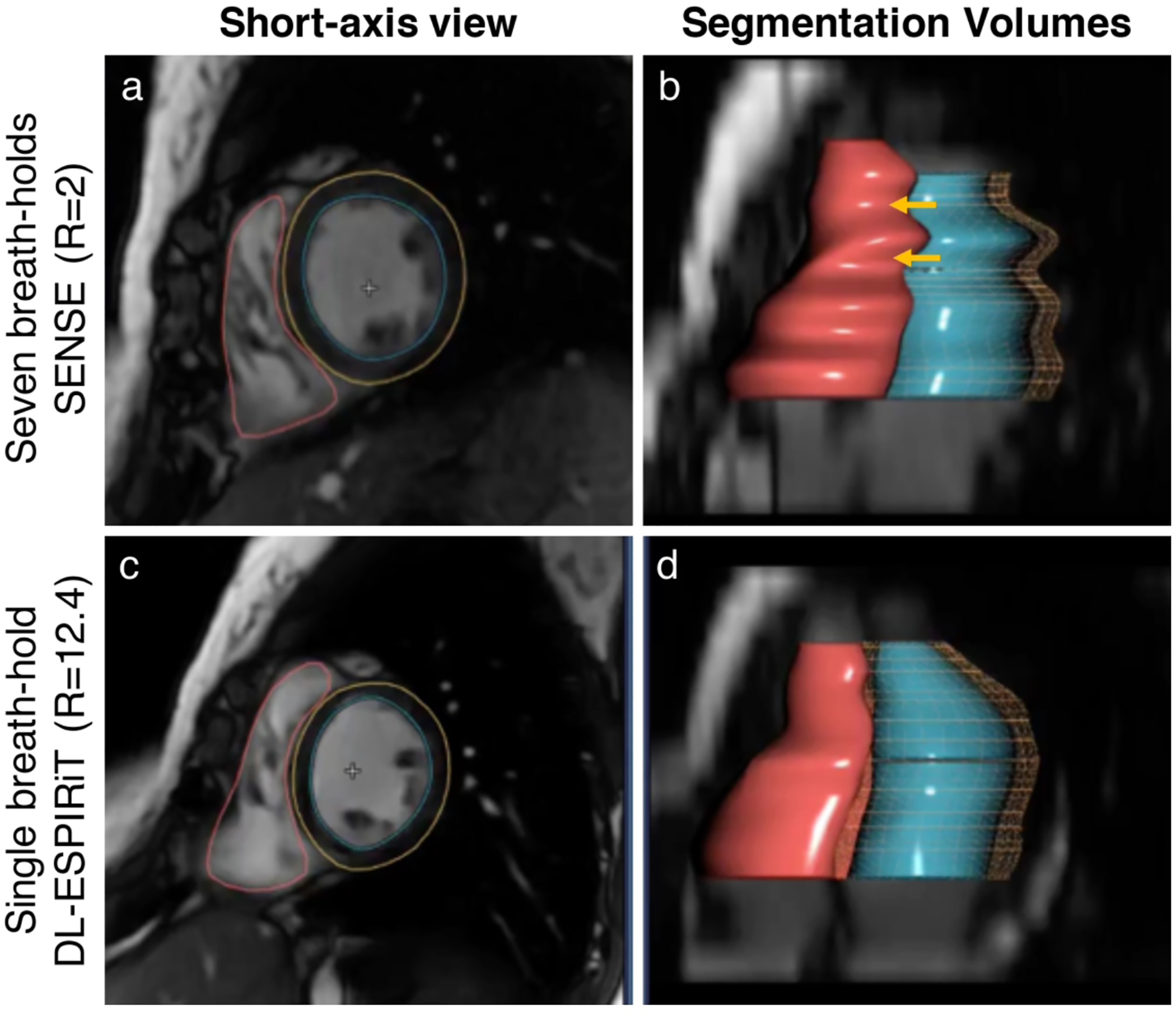
To reduce the total number of breath-holds for 2D cardiac cine, a parallel imaging acquisition is typically used to enable 2-fold scan time acceleration (a). The segmentations of the left ventricular endocardial (blue) and epicardial (yellow) borders, and the right ventricular endocardial border (red) are shown for parallel imaging (b). With model-based DL reconstructions, 12-fold scan time acceleration can be used to achieve single breath-hold scan times without significantly impacted image quality (c). Additionally, DL-accelerated cardiac cine scans can help to reduce inevitable variations between breath-holds which can bias ventricular volume measurements in multi-breath-hold scans (d).

For both model-free and model-based DL tasks, it is important to ensure a framework for real-time reconstruction and quality control of images prior to a patient leaving the imaging facility. If a sequence relies on DL reconstruction or image enhancement and the prospective acquisition of data has image artifacts or is OOD for the trained networks, it is essential to either re-scan the subject with the same protocol or to defer to a protocol that does not rely on the DL post-processing. This necessitates near-real-time inference of the input data in a manner that the MRI technologist or automated algorithm can perform a rough quality-control assessment and choose to re-scan, if necessary. Such a built-in redundancy system may help ensure that patients are not required to return for additional imaging.

Opportunities

Although many works have demonstrated robustness in small cohorts, the robustness of model-based DL reconstructions is not yet fully understood in large, diverse cohorts. Antun et al demonstrated that model-based DL reconstructions can become unstable in the presence of small perturbations and structural changes in the underlying images (68). Using data consistency layers as described above in all models can mitigate the artifacts described in this instability study. Moreover, modeling plausible image corruptions that are likely to arise in real-world deployment instead of simulated patterns that will not arise clinically may provide an increased understanding of the robustness of the method. Opportunities also remain for developing mathematical tools to assess uncertainty in the DL reconstructed images, which can further apprise users of the robustness of the technique (69).

A particularly exciting opportunity that remains for improving model-based DL robustness is the incorporation of other intrinsic signal structures such as complex-valued convolutional layers (70, 71). Most deep learning frameworks do not support complex-valued deep learning and networks generally decompose the real and imaginary components into two separate real-valued channels as inputs into reconstruction models. MRI is inherently complex-valued and conserving phase information is important during reconstruction as well for downstream fat/water separation, phase-contrast imaging, displacement encoding, and quantitative susceptibility mapping applications. In addition, complex-valued convolutional operations have greater expressivity, possibly reducing the number of model parameters and the likelihood of overfitting on training data (70, 71). Novel activation functions such as the zReLU, cReLU, modReLU, and cardioid have been developed for maintaining phase data along with magnitude activations during gradient descent of the DL networks (71, 72). These activations ensure that not only is the network input is complex-valued, but also that the internal representation of the network is complex-valued and consistent with the acquired data (Fig. 6).

Figure 6:

Comparisons of model-based reconstruction networks, with example input zero-filled, real-valued convolutions only, complex-valued convolutions, compressed sensing (CS) with L1-wavelet regularization, and ground truth fully-sampled reconstructions for undersampling factors (R) of 2.3 and 7.40. The difference maps, scaled by a factor of 40, are displayed under each reconstruction. The complex-valued magnitude images appear sharper than the real-valued images and with reduced noise than the CS images. The complex-valued phase maps appear smoother, with red arrows indicating differences in visibility of subtle details.

DL for image reconstruction also provides an additional opportunity to improve the efficiency of reconstruction algorithms. Even if DL algorithms may not surpass image accelerations beyond compressed sensing (CS) for example, training an algorithm to implement CS as a CNN would allow for faster inference durations. Instead of requiring a time-consuming iterative reconstruction, which has limited the clinical impact of CS, a simpler forward pass of a trained CNN could achieve similar reconstructions in near real-time.

Recommendations

Prospective data collection is often necessary for training since most institutions do not store fully-sampled multi-coil k-space data. While large quantities of reconstructed images in DICOM format are stored in hospital databases, the authors recommend that these should not be used for simulating training data. After reconstruction, complex-valued multi-channel images are often interpolated, filtered, coil-combined, converted to magnitude, corrected for gradient non-linearity, and intensity-corrected before being written out as DICOM files. Through these various post-processing steps, valuable information that can be leveraged during the reconstruction, such as phase, is discarded. Moreover, the distribution of training data simulated from DICOM images may differ from that of prospectively collected k-space data, which may impact performance of deployed algorithms. Combining the advances in the representation abilities of CNNs along with physical constraints to which all MRI processes are inherently subjected to, likely improves stability of DL in MRI reconstruction. Using approaches such as data consistency during network training along with the leveraging complex data may enable robust deployment in prospective clinical use-cases.

To address the lack of readily available fully-sampled k-space data, there have been initiatives to collect and release large databases of fully-sampled 2D and 3D fast spin echo k-space data (73, 74). A practical challenge that may arise in sharing raw k-space data, especially in the case of high-resolution multi-coil dynamic imaging, is that of storage capacity. For example, approximately 1500 fully-sampled knee MRI scans from the fastMRI dataset require over 1TB of hard disk capacity (74). Leveraging cloud storage providers that have different pricing options as a function of access rates may help alleviate this challenge. Further, to offset the challenges in formatting and handling of raw k-space data, standardized approaches such as those adopted by the International Society for Magnetic Resonance in Medicine can help facilitate easier data sharing (75). Combining these formats with publicly available databases have not only served to enable development of novel DL image reconstruction frameworks, but also provided baselines to compare performance across different networks, much like ImageNet has done for the computer vision community.

CLASSIFICATION AND SEGMENTATION

Classification is perhaps one of the most common computer vision tasks performed in medical imaging with the advent of DL. Classification tasks can be grouped into two different levels: image-wise and pixel-wise classification, also known as segmentation. The former image-wise method may be used to answer questions such as “Is there a stroke in a brain MRI dataset?” to determine a single variable pertinent to the diagnostic status of the subject from either 2D MRI slices, 3D volumes, or multiple 3D sequences. A recent manuscript even highlighted the use of ultrashort echo-time MRI for evaluating COVID-19 imaging findings, for which DL may be able to assist with patient triage and prognostics predictions (76). Such image-level classification is the fundamental underpinning of computer aided detection (CAD) systems. On the other hand, a pixel-wise classification task may help answer “Which pixels in this brain MRI dataset correspond to a region of stroke?” by determining whether each pixel in a given image belongs to a specific class or not. Such pixel-wise classification, tasks have been used to report or isolate the morphology of specific image features of tissues. Numerous review articles have been published recently that summarize the findings from a variety of classification and segmentation tasks for medical imaging (77), MRI in general (78), as well as specialized MRI applications including musculoskeletal imaging (79, 80), breast imaging (81) and neuroradiology (82). In the following sections, we will critically analyze important considerations prior to deploying such algorithms clinically and will provide a perspective on some unaddressed challenges and opportunities to make a tangible clinical impact.

Training Paradigm:

Unlike model-based reconstructions where a physics-based model can lower the need for training data, classification and segmentation tasks typically require larger training datasets to learn accurate image representations and outcomes. To balance the need for large high-quality annotated datasets for MRI tasks, a primary consideration should be to set a minimum acceptable level for the requisite accuracy of the DL model. While setting a precise threshold can be challenging for many clinical scenarios, an approximate technique could entail comparing the performance of a DL model with that of multiple expert radiologists for the task in question. The goal of such an exercise should be to match the variability among the DL models and the expert radiologists to that of the inter-reader variability among the radiologists. Such an approach was applied in a study evaluating the performance of a DL model to detect tears of the anterior cruciate ligament in the knee (83). In this study, the authors further stratified their findings by including human readers with varying levels of expertise, such as residents, fellows, and experienced attending radiologists.

Once such an acceptable performance level of DL systems is established, the training datasets could be progressively subsampled to demonstrate a relationship between the size of an input training dataset versus the accuracy of the model. Prior studies have shown that the accuracy of DL networks scales with a power-law relationship with the size of the input training datasets, and is consistent amongst tasks in computer vision and natural language processing (84). This finding was further validated in a study for segmenting articular cartilage from knee MRI scans that demonstrated that independent of network architectures, increasing the size of the training dataset can predictably estimate the accuracy of the network using a power-law relationship (Fig. 7) (85). Moreover, this study also demonstrated the accuracy of the network architectures by re-training identical models with random seed initializations, which has further been replicated in natural language processing tasks also (86). Including error bars in the accuracy of the models is an important step in understanding the repeatability of the network to random perturbations, especially if multiple different networks will be trained using transfer learning strategies.

Figure 7:

Segmentation of femoral cartilage from knee double-echo steady-state scans shows that the accuracy of the model on an identical test set evaluated with a Dice Score Coefficient (DSC) follows a power-law relationship with the extent of training data with very high correlation coefficients. A power law function for y=f(x) is defined as y = α*x^β.

Robustness:

In contrast to image synthesis and reconstruction tasks, which receive supervision from local regions of images to reduce blurring, noise, etc; classification and segmentation tasks typically rely on a larger receptive field and require image cues from different non-local regions of the image. This distinction makes it important to ensure that all training images are free of artifact to avoid biasing network representation. In addition, a simulated stress-testing pipeline that mimics common artifacts that will likely be present during prospective deployment could help determine whether the model is appropriate for clinical use. For example, failed breath holds during myocardial infarct imaging and image ringing on brain MRI are common artifacts that may be encountered in clinical and research applications and can help determine the robustness of a segmentation network. Additionally, developing methods for detecting OOD images as described above could also help automatically detect if a particular image may not be suitable for analysis by a given trained network (87).

Downstream Analysis:

The goal of most classification and segmentation systems is to aid the radiologist in making a rapid and accurate diagnostic decision. Thus, to ensure that DL models can be as efficacious as possible, they should be tightly integrated into the routine workflow of a radiology practice. Without integration into the picture archiving and communications systems (PACS), the promise of DL models may not fully be realized because obtaining information from the DL model would require time-consuming consultation with a system that is not a part of routine workflow. Recent guidelines provided through the Integrating the Health Enterprise (IHE) address workflow management and the incorporation of DL algorithms for medical images in clinical settings (88, 89). These encourage the use of common standards such as the DICOM format for imaging data and Fast Healthcare Interoperability Resources (FHIR) for electronic medical record data. They emphasize AI results being presented to radiologists in a standard reading environment in a supplementary manner to existing workflows, taking into account worklist prioritization and continual learning algorithms that learn from previous radiologist-AI shared interactions.

Further, even if a successful and seamless integration with PACS is possible, not enough is known about how the information from models should be presented to the radiologists. Researchers have only recently started to study how best to pair a human expert with a DL classification model (90). In the case of a pathology images, one study showed that when a DL pathology classification model was correct, it increased the aggregate accuracy of 11 pathologists, but when the model was incorrect, it decreased the accuracy of the pathologists, compared to baseline (91). Experiences in interaction between human users and CAD software from mammography may provide powerful lessons in determining how to best integrate decision support tools clinically (92, 93). A recent meta-analysis found that CAD in mammography did not always increase sensitivity of studies and actually decreased specificity in some studies (94). Additionally, compared to radiologists who read large volumes of mammograms, CAD was more beneficial for lower volume readers. These findings suggest that designers of DL CAD models should critically understand the tradeoffs between positive and negative predictive values of models, based on specific use-cases and prospective users. In lower resource or high-volume settings, CAD could also be used as a second reader as a part of double read systems.

Opportunities

A common criticism of DL algorithms, especially those used for image classification, is their ‘black-box’ nature, alluding to the difficulty of users to understand how they function. Unlike traditional signal processing tools, no transfer function or point-spread function can specify the optimal behavior of an arbitrary model for a given set of inputs. To remedy this challenge, concepts such as integrated gradients and saliency maps have been proposed (95, 96). These powerful approaches provide a pixel-wise attribution to estimate how important a particular pixel was for the final model classification. Instead of only performing such interpretability analysis on a few examples from a testing dataset, there lies a large opportunity in performing this technique on the entire training and testing datasets to uncover latent but clinically meaningful relationships. Pairing saliency with uncertainty analysis can also provide additional context and confidence to the interpreting radiologist. Similar to the model-based reconstruction approaches, embedding prior human knowledge with the data-driven capabilities of DL networks may also help achieve high model and decision interpretability.

DL also has an opportunity to show clinical impact by performing entirely in-silico retrospective research studies. When a large external dataset is available, it can be used to show that replacing manual assessments with automated segmentation and classification provides the same study and patient outcomes, thereby enabling model deployment with higher confidence. For example, a prior study showed that an automated segmentation algorithm for thigh muscle areas can replicate effect sizes determined with manual segmentation on a clinical study of subjects experiencing osteoarthritic pain (97). Similarly, DL can further complement and enhance the high-value sequences in MRI studies where automated segmentation methods can be used for analysis of the entire imaging volumes, instead of single slices only (98).

In such clinical and research studies, there are often circumstances when either a longitudinal timepoint or a specific scan sequence is missing from the overall analysis. DL models can be made robust to such incomplete datasets by augmenting training datasets by randomly excluding network inputs. Such an approach, termed DropOut, which randomly excluded MRI sequences during network training for segmenting brain metastasis showed superior results compared to an approach that used complete MRI contrasts (Fig. 8) (99).

Figure 8:

Case examples from a post-gadolinium-enhanced T1-weighted image series (a) for the MRI sequence DropOut method showing the segmentation predictions using (b) DeepLab V3 and (c) the proposed method. Segmentation predictions are shown as voxel-wise probability maps (ranging from 0.5 to 1) and performance maps classified as true negative, false positive, and false negative as specified by the color code. The first row shows a 53-year-old female patient with malignant melanoma, while the second and third row show a 55-year-old female with malignant melanoma. The arrows indicate true positive lesions (blue) and false positive lesions (yellow). Note that in the last row, the DeepLab V3 show false positive lesions which are not reported by the DropOut method. Figure courtesy Dr. Endre Grøvik from the ongoing TREATMENT clinical study (NCT03458455).

Recommendations

For determining beneficial use cases for MRI classification and segmentation, we recommend developing a robust pipeline to ensure that common MRI artifacts do not cause networks to perceive real-world images as OOD. By sub-sampling the training data, the amount necessary for the given clinical task may be coarsely extrapolated. This extrapolation can support an analysis to ensure that all studies using DL are adequately powered to detect subtle changes. Developing approaches to quantify the uncertainty of model outputs also can help radiologists during image interpretation (100, 101). Combining multiple models for classification and segmentation models tailored to specific clinical protocols may also assist in differential diagnoses for radiologists, as was demonstrated in the case of neuroradiology (102).

Lastly, Occam’s Razor suggests that when multiple models are being used for a downstream task, the best approach is to use the model with the fewest assumptions. Especially with newer DL models using millions of trainable free parameters, developing the simplest models may provide the best results for troubleshooting and during implementation. A study of a segmentation challenge organized in 2019 showed that simpler models often perform on par with larger and more complex models (103).

REPRODUCIBILITY:

One of the largest differences between computer vision for natural imaging and for medical imaging, is likely that of reproducible experiments. This difference can be further broken down into reproducible data and reproducible experimental setups. The computer vision community in natural imaging has flourished due to the existence of large scale datasets such as ImageNet, Microsoft Common Objects in Context (MS-COCO), etc (104, 105). Concerns with patient health information and adequate anonymization techniques make data sharing of MRI considerably more challenging than in natural imaging. However, the presence of large-scale efforts such as those in fastMRI and MRNet that provide high-quality data with appropriate annotations (fully-sampled k-space for fastMRI and acute injuries for knee MRI in MRNet) are encouraging efforts for the entire research community (74, 106). While sharing of datasets is essential to advance the DL in medical imaging community as whole, sharing of data must be governed with a strong ethical conduct (107).

Although sharing of code faces much fewer hurdles than sharing data, it is still uncommon, with only a handful of publications openly releasing software resources. Code sharing can create a powerful generalized framework for the entire research community, both to replicate experiments with varying datasets and to improve the speed and efficiency of research. Furthermore, since DL can involve a large variety of hyperparameters, there is a significant need for improved and standardized reporting of the procedures used to train DL algorithms. The recently developed Checklist for Artificial Intelligence in Medical Imaging (CLAIM) checklist provides a solid foundation for encouraging adequate reporting of parameters (108). Going further than CLAIM, we recommend that all manuscripts also report their hyperparameter optimization strategies, along with a summary of which parameters were successful and which were not. Reporting unsuccessful parameters can help other researchers avoid similar mistakes and can mitigate the economic and environmental impacts of machine learning research (109). For DL to advance into the clinic faster, such code and data sharing practices should have a higher priority than they do currently.

CONCLUSION AND SUMMARY

Deep learning has the potential to improve every step of the MRI diagnostic workflow and to provide value for every user, all the way from the technologists performing the scan, the physician ordering the imaging, the radiologist providing the interpretation, and most importantly, the patient who is receiving the medical care. Before these benefits are realized, there is a pressing need to systematically characterize the robustness of our current deep learning processes and to improve our understanding of the success and failure modes of these algorithms. We have addressed some of the major challenges to bridge the gap between technology development in deep learning and clinical deployment of these methods.

Our overview of DL applications in MRI focused on techniques that have potential and utility for clinical deployment. We paired these techniques with a framework for important considerations prior to the beginning of new deep learning studies in order to fully understand key questions and the challenges that can arise in the deployment of these tools. We hope that by summarizing the current challenges and opportunities, by and recommending best practices for the use of deep learning, MRI becomes an even higher-value modality.

Table 1:

A summary of the framework for the analysis of deep leaming (DL) algorithms for the application areas of model-free image synthesis, model-based reconstruction, and classification and segmentation problems.

	Model-Free Image Synthesis	Model-Based Reconstruction	Classification and Segmentation
Training Paradigm	• Creation of paired datasets • Guarding against hallucinations or missing details	• Choice of appropriate loss functions • Challenge in acquiring fully sampled data	• Understanding the accuracy necessary for clinical task • Determining an adequate sample size for required accuracy • Impact of random seeds
Robustness	• Adversarial robustness • Out-of-domain detection	• Incorporation of data consistency and physics-embeddings into models	• Adversarial robustness to commonly experienced imaging artifacts
Downstream Analysis	• Biases in diagnoses and tissue quantification	• Accurate quantification and interpretation of images • Real-time inference for quality-control and minimizing call-backs	• Integration into routine clinical workflow • Evaluation how to best present outputs
Opportunitles	• Quantitation of perceptual image quality mètrics • Blind image quality mètrics • Improveddata augmentations	• Model uncertainty and adversarial robustness • Use of complex-valued neural networks • Speeding up iterative reconstruction processes	• Going beyond analysis of saliency on single test images • Performing in-silico studies to determine similarity of outcomes • Guard against missing input images
Recommendations	• Demonstrating models on prospective real-world data	• Using complex-valued input data with complex convolutional layers and data consistency	• Developing simulation pipeline to improve robustness to OOD data • Using the simplest model

REFERENCES:

- 1.Greenspan H, van Ginneken B, Summers RM: Guest Editorial Deep Learning in Medical Imaging: Overview and Future Promise of an Exciting New Technique. IEEE Trans Med Imaging 2016; 35:1153–1159. [Google Scholar]
- 2.Lundervold AS, Lundervold A: An overview of deep learning in medical imaging focusing on MRI. Z Med Phys 2019; 29:102–127. [DOI] [PubMed] [Google Scholar]
- 3.LeCun Y, Bengio Y, Hinton G: Deep learning. Nature 2015; 521:436–444. [DOI] [PubMed] [Google Scholar]
- 4.FDA Cleared AI Algorithms [Google Scholar]
- 5.Lin DJ, Johnson PM, Knoll F, Lui YW: Artificial Intelligence for MR Image Reconstruction: An Overview for Clinicians. J Magn Reson Imaging 2020:1–14. [DOI] [PMC free article] [PubMed] [Google Scholar]
- 6.Chartrand G, Cheng PM, Vorontsov E, et al. : Deep Learning: A Primer for Radiologists. RadioGraphics 2017; 37:2113–2131. [DOI] [PubMed] [Google Scholar]
- 7.Soffer S, Ben-Cohen A, Shimon O, Amitai MM, Greenspan H, Klang E: Convolutional Neural Networks for Radiologic Images: A Radiologist’s Guide. Radiology 2019; 290:590–606. [DOI] [PubMed] [Google Scholar]
- 8.Xu Y, Mo T, Feng Q, Zhong P, Lai M, Chang EI: Deep learning of feature representation with multiple instance learning for medical image analysis. In 2014 IEEE Int Conf Acoust Speech Signal Process. IEEE; 2014:1626–1630. [Google Scholar]
- 9.Olah C, Mordvintsev A, Schubert L: Feature Visualization. Distill 2017; 2. [Google Scholar]
- 10.Van Reeth E, Tham IIWK, Tan CH, Poh CL, Reeth E Van, Tham IIWK: Super-resolution in magnetic resonance imaging: A review. Concepts Magn Reson Part A 2012; 40:306–325. [Google Scholar]
- 11.Chaudhari AS, Fang Z, Kogan F, et al. : Super-resolution musculoskeletal MRI using deep learning. Magn Reson Med 2018; 80:2139–2154. [DOI] [PMC free article] [PubMed] [Google Scholar]
- 12.Chen Y, Xie Y, Zhou Z, Shi F, Christodoulou AG, Li D: Brain MRI super resolution using 3D deep densely connected neural networks. In 2018 IEEE 15th Int Symp Biomed Imaging (ISBI 2018). Volume 2018-April. IEEE; 2018(Isbi):739–742. [Google Scholar]
- 13.Benou A, Veksler R, Friedman A, Riklin Raviv T: Ensemble of expert deep neural networks for spatio-temporal denoising of contrast-enhanced MRI sequences. Med Image Anal 2017; 42:145–159. [DOI] [PubMed] [Google Scholar]
- 14.Lehtinen J, Munkberg J, Hasselgren J, et al. : Noise2Noise: Learning image restoration without clean data. 35th Int Conf Mach Learn ICML 2018 2018; 7:4620–4631. [Google Scholar]
- 15.Gibbons EK, Hodgson KK, Chaudhari AS, et al. : Simultaneous NODDI and GFA parameter map generation from subsampled q-space imaging using deep learning. Magn Reson Med 2019; 81:2399–2411. [DOI] [PubMed] [Google Scholar]
- 16.Tian Q, Bilgic B, Fan Q, Liao C, Ngamsombat C: DeepDTI: High-fidelity six-direction diffusion tensor imaging using deep learning. Neuroimage 2020:117017. [DOI] [PMC free article] [PubMed] [Google Scholar]
- 17.Golkov V, Dosovitskiy A, Sperl JI, et al. : q-Space Deep Learning: Twelve-Fold Shorter and Model-Free Diffusion MRI Scans. IEEE Trans Med Imaging 2016; 35:1344–1351. [DOI] [PubMed] [Google Scholar]
- 18.Zeng DY, Shaikh J, Holmes S, et al. : Deep residual network for off-resonance artifact correction with application to pediatric body MRA with 3D cones. Magn Reson Med 2019; 82:1398–1411. [DOI] [PMC free article] [PubMed] [Google Scholar]
- 19.Küstner T, Armanious K, Yang J, Yang B, Schick F, Gatidis S: Retrospective correction of motion-affected MR images using deep learning frameworks. Magn Reson Med 2019; 82:1527–1540. [DOI] [PubMed] [Google Scholar]
- 20.Zhang Q, Ruan G, Yang W, et al. : MRI Gibbs-ringing artifact reduction by means of machine learning using convolutional neural networks. Magn Reson Med 2019; 82:2133–2145. [DOI] [PubMed] [Google Scholar]
- 21.Leynes AP, Yang J, Wiesinger F, et al. : Zero-echo-time and dixon deep pseudo-CT (ZeDD CT): Direct generation of pseudo-CT images for Pelvic PET/MRI Attenuation Correction Using Deep Convolutional Neural Networks with Multiparametric MRI. J Nucl Med 2018; 59:852–858. [DOI] [PMC free article] [PubMed] [Google Scholar]
- 22.Kearney V, Ziemer BP, Perry A, et al. : Attention-Aware Discrimination for MR-to-CT Image Translation Using Cycle-Consistent Generative Adversarial Networks. Radiol Artif Intell 2020; 2:e190027. [DOI] [PMC free article] [PubMed] [Google Scholar]
- 23.Gong E, Pauly JM, Wintermark M, Zaharchuk G: Deep learning enables reduced gadolinium dose for contrast-enhanced brain MRI. J Magn Reson Imaging 2018; 48:330–340. [DOI] [PubMed] [Google Scholar]
- 24.Kleesiek J, Morshuis JN, Isensee F, et al. : Can Virtual Contrast Enhancement in Brain MRI Replace Gadolinium?: A Feasibility Study. Invest Radiol 2019; 54:653–660. [DOI] [PubMed] [Google Scholar]
- 25.Cohen JP, Luck M, Honari S: Distribution matching losses can hallucinate features in medical image translation. Med Image Comput Comput Assist Interv – MICCAI 2018; 11070 LNCS:529–536. [Google Scholar]
- 26.He K, Zhang X, Ren S, Sun J: Deep residual learning for image recognition. Proc IEEE Comput Soc Conf Comput Vis Pattern Recognit 2016; 2016-Decem:770–778. [Google Scholar]
- 27.Kim J, Kwon Lee J, Mu Lee K, Lee JK, Lee KM: Accurate Image Super-Resolution Using Very Deep Convolutional Networks. Cvpr 2016. 2016:1646–1654. [Google Scholar]
- 28.Zaeemzadeh A, Rahnavard N, Shah M: Norm-Preservation: Why Residual Networks Can Become Extremely Deep? IEEE Trans Pattern Anal Mach Intell 2020; 8828(c):1–1. [DOI] [PubMed] [Google Scholar]
- 29.Cortes C, Mohri M, Rostamizadeh A: L2 regularization for learning kernels. Proc 25th Conf Uncertain Artif Intell UAI 2009 2009:109–116. [Google Scholar]
- 30.Pham CH, Ducournau A, Fablet R, Rousseau F: Brain MRI super-resolution using deep 3D convolutional networks. Proc - Int Symp Biomed Imaging 2017:197–200. [Google Scholar]
- 31.Huang S, Papernot N, Goodfellow I, et al. : Adversarial Attacks on Neural Network Policies. 5th Int Conf Learn Represent ICLR 2017 - Work Proc 2017:1–7. [Google Scholar]
- 32.Hendrycks D, Gimpel K: A baseline for detecting misclassified and out-of-distribution examples in neural networks. 5th Int Conf Learn Represent ICLR 2017 - Conf Track Proc 2017:1–12. [Google Scholar]
- 33.Knoll F, Hammernik K, Kobler E, Pock T, Recht MP, Sodickson DK: Assessment of the Generalization of Learned Image Reconstruction and the Potential for Transfer Learning. Magn Reson Med 2019; 81:116–128. [DOI] [PMC free article] [PubMed] [Google Scholar]
- 34.Wang Z, Bovik AC, Sheikh HR and Simoncelli EP: Wavelets for Image Image quality assessment: From error visibility to structural similarity. IEEE Trans Image Process 2004; 13:600–612. [DOI] [PubMed] [Google Scholar]
- 35.Ghodrati V, Shao J, Bydder M, et al. : MR image reconstruction using deep learning: Evaluation of network structure and loss functions. Quant Imaging Med Surg 2019; 9:1516–1527. [DOI] [PMC free article] [PubMed] [Google Scholar]
- 36.Knoll F, Murrell T, Sriram A, et al. : Advancing machine learning for MR image reconstruction with an open competition: Overview of the 2019 fastMRI challenge. Magn Reson Med 2020(April):mrm.28338. [DOI] [PMC free article] [PubMed] [Google Scholar]
- 37.Oktay O, Ferrante E, Kamnitsas K, et al. : Anatomically Constrained Neural Networks (ACNNs): Application to Cardiac Image Enhancement and Segmentation. IEEE Trans Med Imaging 2018; 37:384–395. [DOI] [PubMed] [Google Scholar]
- 38.Chaudhari AS, Stevens KJ, Wood JP, et al. : Utility of deep learning super-resolution in the context of osteoarthritis MRI biomarkers. J Magn Reson Imaging 2020; 51:768–779. [DOI] [PMC free article] [PubMed] [Google Scholar]
- 39.Chaudhari A, Fang Z, Lee JH, Gold G, Hargreaves B: Deep Learning Super-Resolution Enables Rapid Simultaneous Morphological and Quantitative Magnetic Resonance Imaging. In Int Work Mach Learn Med Image Reconstr; 2018:3–11. [Google Scholar]
- 40.Chaudhari AS, Grissom M, Sveinsson B, et al. : Diagnostic Accuracy of Quantitative Multi-Contrast 5-Minute Knee MRI Using Prospective Artificial Intelligence Image Quality Enhancement Title. Am J Roentgenol 2020; (in press). [DOI] [PMC free article] [PubMed] [Google Scholar]
- 41.Zhang R, Isola P, Efros AA, Shechtman E, Wang O: The Unreasonable Effectiveness of Deep Features as a Perceptual Metric. In 2018 IEEE/CVF Conf Comput Vis Pattern Recognit. IEEE; 2018:586–595. [Google Scholar]
- 42.Johnson J, Alahi A, Fei-Fei L: Perceptual losses for real-time style transfer and super-resolution. Lect Notes Comput Sci (including Subser Lect Notes Artif Intell Lect Notes Bioinformatics) 2016; 9906 LNCS:694–711. [Google Scholar]
- 43.Zhu JY, Park T, Isola P, Efros AA: Unpaired Image-to-Image Translation Using Cycle-Consistent Adversarial Networks. Proc IEEE Int Conf Comput Vis 2017; 2017-Octob:2242–2251. [Google Scholar]
- 44.Zhu B, Liu JZ, Cauley SF, Rosen BR, Rosen MS: Image Reconstruction by Domain-Transform Manifold Learning. Nature 2018; 555:487–492. [DOI] [PubMed] [Google Scholar]
- 45.Lee D, Yoo J, Ye JC: Deep residual learning for compressed sensing MRI. In 2017 IEEE 14th Int Symp Biomed Imaging (ISBI 2017). IEEE; 2017:15–18. [Google Scholar]
- 46.Mardani M, Gong E, Cheng JY, et al. : Deep Generative Adversarial Neural Networks for Compressive Sensing MRI. IEEE Trans Med Imaging 2019; 38:167–179. [DOI] [PMC free article] [PubMed] [Google Scholar]
- 47.Liu F, Samsonov A, Chen L, Kijowski R, Feng L: SANTIS: Sampling-Augmented Neural neTwork with Incoherent Structure for MR image reconstruction. Magn Reson Med 2019; 82:1890–1904. [DOI] [PMC free article] [PubMed] [Google Scholar]
- 48.Hauptmann A, Arridge S, Lucka F, Muthurangu V, Steeden JA: Real-time cardiovascular MR with spatio-temporal artifact suppression using deep learning–proof of concept in congenital heart disease. Magn Reson Med 2019; 81:1143–1156. [DOI] [PMC free article] [PubMed] [Google Scholar]
- 49.Yang Y, Sun J, Li H, Xu Z: ADMM-Net: A Deep Learning Approach for Compressive Sensing MRI. In Adv {{Neural Inf Process Syst 29. Edited by Lee DD, Sugiyama M, Luxburg UV, Guyon I, Garnett R. Curran Associates, Inc.; 2016:10–18. [Google Scholar]
- 50.Hammernik K, Klatzer T, Kobler E, et al. : Learning a variational network for reconstruction of accelerated MRI data. Magn Reson Med 2018; 79:3055–3071. [DOI] [PMC free article] [PubMed] [Google Scholar]
- 51.Schlemper J, Caballero J, Hajnal JV, Price A, Rueckert D: A Deep Cascade of Convolutional Neural Networks for MR Image Reconstruction. In IEEE Trans Med Imaging. Volume 37; 2017:647–658. [DOI] [PubMed] [Google Scholar]
- 52.Aggarwal HK, Mani MP, Jacob M: MoDL: Model-Based Deep Learning Architecture for Inverse Problems. IEEE Trans Med Imaging 2019; 38:394–405. [DOI] [PMC free article] [PubMed] [Google Scholar]
- 53.Sandino CM, Cheng JY, Chen F, Mardani M, Pauly JM, Vasanawala SS: Compressed Sensing: From Research to Clinical Practice With Deep Neural Networks: Shortening Scan Times for Magnetic Resonance Imaging. IEEE Signal Process Mag 2020; 37:117–127. [DOI] [PMC free article] [PubMed] [Google Scholar]
- 54.Chen F, Taviani V, Malkiel I, et al. : Variable-Density Single-Shot Fast Spin-Echo MRI with Deep Learning Reconstruction by Using Variational Networks. Radiology 2018; 289:366–373. [DOI] [PMC free article] [PubMed] [Google Scholar]
- 55.Zhao H, Gallo O, Frosio I, Kautz J: Loss Functions for Image Restoration With Neural Networks. IEEE Trans Comput Imaging 2017; 3:47–57. [Google Scholar]
- 56.Seitzer M, Yang G, Schlemper J, et al. : Adversarial and Perceptual Refinement for Compressed Sensing MRI Reconstruction. In Med Image Comput Comput Assist Interv; 2018:232–240. [Google Scholar]
- 57.Akçakaya M, Moeller S, Weingärtner S, Uğurbil K: Scan-specific robust artificial-neural-networks for k-space interpolation (RAKI) reconstruction: Database-free deep learning for fast imaging. Magn Reson Med 2019; 81:439–453. [DOI] [PMC free article] [PubMed] [Google Scholar]
- 58.Tamir JI, Yu SX, Lustig M: Unsupervised Deep Basis Pursuit: Learning inverse problems without ground-truth data. arXiv:191013110 [eess] 2020. [Google Scholar]
- 59.Lei K, Mardani M, Pauly JM, Vasanawala SS: Wasserstein GANs for MR Imaging: from Paired to Unpaired Training. arXiv191007048 [cs, eess] 2020. [DOI] [PMC free article] [PubMed] [Google Scholar]
- 60.Cole EK, Ong F, Pauly JM, Vasanawala SS: Unsupervised Image Reconstruction using Deep Generative Adversarial Networks. In ISMRM Work Data Sampl Image Reconstr. Sedona, AZ, USA; 2020. [Google Scholar]
- 61.Krizhevsky A, Sutskever I, Hinton GE: ImageNet Classification with Deep Convolutional Neural Networks. Adv Neural Inf Process Syst 2012:1–9. [Google Scholar]
- 62.Vishnevskiy V, Walheim J, Kozerke S: Deep variational network for rapid 4D flow MRI reconstruction. Nat Mach Intell 2020; 2:228–235. [Google Scholar]
- 63.Dar SUH, Özbey M, Çatlı AB, Çukur T: A Transfer-Learning Approach for Accelerated MRI Using Deep Neural Networks. Magn Reson Med 2020; 84:663–685. [DOI] [PubMed] [Google Scholar]
- 64.Liu F, Feng L, Kijowski R: MANTIS: Model-Augmented Neural neTwork with Incoherent k-space Sampling for efficient MR parameter mapping. Magn Reson Med 2019; 82:174–188. [DOI] [PMC free article] [PubMed] [Google Scholar]
- 65.Chaudhari AS, Stevens KJ, Sveinsson B, et al. : Combined 5-minute double-echo in steady-state with separated echoes and 2-minute proton-density-weighted 2D FSE sequence for comprehensive whole-joint knee MRI assessment. J Magn Reson Imaging 2019; 49:e183–e194. [DOI] [PMC free article] [PubMed] [Google Scholar]
- 66.Chaudhari AS, Black MS, Eijgenraam S, et al. : Five-minute knee MRI for simultaneous morphometry and T 2 relaxometry of cartilage and meniscus and for semiquantitative radiological assessment using double-echo in steady-state at 3T. J Magn Reson Imaging 2018; 47:1328–1341. [DOI] [PMC free article] [PubMed] [Google Scholar]
- 67.Sandino CM, Lai P, Vasanawala SS, Cheng JY: Accelerating Cardiac Cine MRI Using a Deep Learning-Based ESPIRiT Reconstruction. arXiv191105845 [cs, eess] 2020. [DOI] [PMC free article] [PubMed] [Google Scholar]
- 68.Antun V, Renna F, Poon C, Adcock B, Hansen AC: On instabilities of deep learning in image reconstruction and the potential costs of AI. Proc Natl Acad Sci 2020:201907377. [DOI] [PMC free article] [PubMed] [Google Scholar]
- 69.Edupuganti V, Mardani M, Vasanawala S, Pauly J: Uncertainty Quantification in Deep MRI Reconstruction. arXiv190111228 [cs] 2020. [DOI] [PMC free article] [PubMed] [Google Scholar]
- 70.Trabelsi C, Bilaniuk O, Zhang Y, et al. : Deep Complex Networks. In Int Conf Learn Represent; 2018. [Google Scholar]
- 71.Cole EK, Cheng JY, Pauly JM, Vasanawala SS: Analysis of Deep Complex-Valued Convolutional Neural Networks for MRI Reconstruction. arXiv:200401738 [physics] 2020. [DOI] [PMC free article] [PubMed] [Google Scholar]
- 72.Arjovsky M, Shah A, Bengio Y: Unitary Evolution Recurrent Neural Networks. In Proc 33rd Int Conf Mach Learn. Volume 48. Edited by Balcan MF, Weinberger KQ. New York, New York, USA: PMLR; 2016:1120–1128. [Proceedings of Machine Learning Research] [Google Scholar]
- 73.Ong F, Amin S, Vasanawala SS, Lustig M: An Open Archive for Sharing MRI Raw Data. In Int Soc Magn Reson Med. Paris, France; 2018. [Google Scholar]
- 74.Knoll F, Zbontar J, Sriram A, et al. : fastMRI: A Publicly Available Raw k-Space and DICOM Dataset of Knee Images for Accelerated MR Image Reconstruction Using Machine Learning. Radiol Artif Intell 2020; 2:e190007. [DOI] [PMC free article] [PubMed] [Google Scholar]
- 75.Inati SJ, Naegele JD, Zwart NR, et al. : ISMRM Raw data format: A proposed standard for MRI raw datasets. Magn Reson Med 2017; 77:411–421. [DOI] [PMC free article] [PubMed] [Google Scholar]
- 76.Yang S, Zhang Y, Shen J, et al. : Clinical Potential of UTE-MRI for Assessing COVID-19: Patient- and Lesion-Based Comparative Analysis. J Magn Reson Imaging 2020:397–406. [DOI] [PMC free article] [PubMed] [Google Scholar]
- 77.Litjens G, Kooi T, Bejnordi BE, et al. : A survey on deep learning in medical image analysis. Med Image Anal 2017; 42(December 2012):60–88. [DOI] [PubMed] [Google Scholar]
- 78.Mazurowski MA, Buda M, Saha A, Bashir MR: Deep learning in radiology: An overview of the concepts and a survey of the state of the art with focus on MRI. J Magn Reson Imaging 2019; 49:939–954. [DOI] [PMC free article] [PubMed] [Google Scholar]
- 79.Chaudhari AS, Kogan F, Pedoia V, Majumdar S, Gold GE, Hargreaves BA: Rapid Knee MRI Acquisition and Analysis Techniques for Imaging Osteoarthritis. J Magn Reson Imaging 2019:jmri.26991. [DOI] [PMC free article] [PubMed] [Google Scholar]
- 80.Gyftopoulos S, Lin D, Knoll F, Doshi AM, Rodrigues TC, Recht MP: Artificial Intelligence in Musculoskeletal Imaging: Current Status and Future Directions. Am J Roentgenol 2019(September):1–8. [DOI] [PMC free article] [PubMed] [Google Scholar]
- 81.Sheth D, Giger ML: Artificial intelligence in the interpretation of breast cancer on MRI. J Magn Reson Imaging 2020; 51:1310–1324. [DOI] [PubMed] [Google Scholar]
- 82.Yao AD, Cheng DL, Pan I, Kitamura F: Deep Learning in Neuroradiology: A Systematic Review of Current Algorithms and Approaches for the New Wave of Imaging Technology. Radiol Artif Intell 2020; 2:e190026. [DOI] [PMC free article] [PubMed] [Google Scholar]
- 83.Liu F, Guan B, Zhou Z, et al. : Fully Automated Diagnosis of Anterior Cruciate Ligament Tears on Knee MR Images by Using Deep Learning. Radiol Artif Intell 2019; 1:180091. [DOI] [PMC free article] [PubMed] [Google Scholar]
- 84.Hestness J, Narang S, Ardalani N, et al. : Deep Learning Scaling is Predictable, Empirically. 2017:1–19. [Google Scholar]
- 85.Desai A, Gold G, Hargreaves B, Chaudhari A: Technical Considerations for Semantic Segmentation in MRI using Convolutional Neural Networks. arXiv Prepr arXiv190201977 2019. [Google Scholar]
- 86.Dodge J, Ilharco G, Schwartz R, Farhadi A, Hajishirzi H, Smith N: Fine-Tuning Pretrained Language Models: Weight Initializations, Data Orders, and Early Stopping. arXiv Prepr arXiv 2002 06305 2020. [Google Scholar]
- 87.Lee K, Lee K, Lee H, Shin J: A simple unified framework for detecting out-of-distribution samples and adversarial attacks. Adv Neural Inf Process Syst 2018; 2018-Decem(LID):7167–7177. [Google Scholar]
- 88.Radiology Technical Committee: Imaging, AI Workflow for AIW-I. IHE Radiol Tech Framew Suppl 2020; Revision 1. [Google Scholar]
- 89.Radiology Technical Committee: AI Results (AIR). IHE Radiol Tech Framew Suppl 2020; Revision 1. [Google Scholar]
- 90.Patel BN, Rosenberg L, Willcox G, et al. : Human–machine partnership with artificial intelligence for chest radiograph diagnosis. npj Digit Med 2019; 2. [DOI] [PMC free article] [PubMed] [Google Scholar]
- 91.Kiani A, Uyumazturk B, Rajpurkar P, et al. : Impact of a deep learning assistant on the histopathologic classification of liver cancer. npj Digit Med 2020; 3:1–8. [DOI] [PMC free article] [PubMed] [Google Scholar]
- 92.Alberdi E, Povyakalo A, Strigini L, Ayton P: Effects of incorrect computer-aided detection (CAD) output on human decision-making in mammography. Acad Radiol 2004; 11:909–918. [DOI] [PubMed] [Google Scholar]
- 93.Balleyguier C, Kinkel K, Fermanian J, et al. : Computer-aided detection (CAD) in mammography: Does it help the junior or the senior radiologist? Eur J Radiol 2005; 54:90–96. [DOI] [PubMed] [Google Scholar]
- 94.Henriksen EL, Carlsen JF, Vejborg IMM, Nielsen MB, Lauridsen CA: The efficacy of using computer-aided detection (CAD) for detection of breast cancer in mammography screening: a systematic review. Acta radiol 2019; 60:13–18. [DOI] [PubMed] [Google Scholar]
- 95.Sundararajan M, Taly A, Yan Q: Axiomatic attribution for deep networks. 34th Int Conf Mach Learn ICML 2017 2017; 7:5109–5118. [Google Scholar]
- 96.Zhao R, Ouyang W, Li H, Wang X: Saliency detection by multi-context deep learning. Proc IEEE Comput Soc Conf Comput Vis Pattern Recognit 2015; 07–12-June:1265–1274. [Google Scholar]
- 97.Kemnitz J, Baumgartner CF, Eckstein F, et al. : Clinical evaluation of fully automated thigh muscle and adipose tissue segmentation using a U-Net deep learning architecture in context of osteoarthritic knee pain. Magn Reson Mater Physics, Biol Med 2019. [DOI] [PMC free article] [PubMed] [Google Scholar]
- 98.Eijgenraam SM, Chaudhari AS, Reijman M, et al. : Time-saving opportunities in knee osteoarthritis: T2 mapping and structural imaging of the knee using a single 5-min MRI scan. Eur Radiol 2020; 30:2231–2240. [DOI] [PMC free article] [PubMed] [Google Scholar]
- 99.Grøvik E, Yi D, Iv M, et al. : Handling Missing MRI Input Data in Deep Learning Segmentation of Brain Metastases: A Multi-Center Study. arXiv : 1912:11966 2019. [Google Scholar]
- 100.Baumgartner CF, Tezcan KC, Chaitanya K, et al. : PHiSeg: Capturing Uncertainty in Medical Image Segmentation. In Med Image Comput Comput Assist Interv; 2019:119–127. [Google Scholar]
- 101.Gal Y, Ghahramani Z: Dropout As a Bayesian Approximation: Representing Model Uncertainty in Deep Learning. In Proc 33rd Int Conf Int Conf Mach Learn - Vol 48; 2016:1050–1059. [Google Scholar]
- 102.Rauschecker AM, Rudie JD, Xie L, Wang J, Gee JC: Neuroradiologist-level Differential Diagnosis Accuracy at Brain MRI. 2020. [DOI] [PMC free article] [PubMed]
- 103.Desai AD, Caliva F, Iriondo C, et al. : The International Workshop on Osteoarthritis Imaging Knee MRI Segmentation Challenge: A Multi-Institute Evaluation and Analysis Framework on a Standardized Dataset. arXiv : 2004:14003 2020. [DOI] [PMC free article] [PubMed] [Google Scholar]
- 104.Deng J, Dong W, Socher R, Li L-J, Kai Li, Li Fei-Fei: ImageNet: A large-scale hierarchical image database. In 2009 IEEE Conf Comput Vis Pattern Recognit. IEEE; 2009:248–255. [Google Scholar]
- 105.Lin T-Y, Maire M, Belongie S, et al. : Microsoft COCO: Common Objects in Context. In Eur Conf Comput Vis; 2014:740–755. [Google Scholar]
- 106.Bien N, Rajpurkar P, Ball RL, et al. : Deep-learning-assisted diagnosis for knee magnetic resonance imaging: Development and retrospective validation of MRNet. PLoS Med 2018; 15:1–19. [DOI] [PMC free article] [PubMed] [Google Scholar]
- 107.Larson DB, Magnus DC, Lungren MP, Shah NH, Langlotz CP: Ethics of using and sharing clinical imaging data for artificial intelligence: A proposed framework. Radiology 2020; 295:675–682. [DOI] [PubMed] [Google Scholar]
- 108.Mongan J, Moy L, Kahn CE: Checklist for Artificial Intelligence and Medical Imaging (Claim). Radiol Artif Intell 2020. [DOI] [PMC free article] [PubMed] [Google Scholar]
- 109.Strubell E, Ganesh A, McCallum A: Energy and policy considerations for deep learning in NLP. ACL 2019 – 57th Annu Meet Assoc Comput Linguist Proc Conf 2020:3645–3650. [Google Scholar]