A Novel Method for Quantitative Analysis of C-Reactive Protein Lateral Flow Immunoassays Images via CMOS Sensor and Recurrent Neural Networks

Abstract

Objective: To design and implement an easy-to-use, Point-of-Care (PoC) lateral flow immunoassays (LFA) reader and data analysis system, which provides a more in-depth quantitative analysis for LFA images than conventional approaches thereby supporting efficient decision making for potential early risk assessment of cardiovascular disease (CVD). Methods and procedures: A novel end-to-end system was developed including a portable device with CMOS camera integrated with optimized illumination and optics to capture the LFA images produced using high-sensitivity C-Reactive Protein (hsCRP) (concentration level < 5 mg/L). The images were transmitted via WiFi to a back-end server system for image analysis and classification. Unlike common image classification approaches which are based on averaging image intensity from a region-of-interest (ROI), a novel approach was developed which considered the signal along the sample’s flow direction as a time series and, consequently, no need for ROI detection. Long Short-Term Memory (LSTM) networks were deployed for multilevel classification. The features based on Dynamic Time Warping (DTW) and histogram bin counts (HBC) were explored for classification. Results: For the classification of hsCRP, the LSTM outperformed the traditional machine learning classifiers with or without DTW and HBC features performed the best (with mean accuracy of 94%) compared to other features. Application of the proposed method to human plasma also suggests that HBC features from LFA time series performed better than the mean from ROI and raw LFA data. Conclusion: As a proof of concept, the results demonstrate the capability of the proposed framework for quantitative analysis of LFA images and suggest the potential for early risk assessment of CVD. Clinical impact: The hsCRP levels < 5 mg/L were aligned with clinically actionable categories for early risk assessment of CVD. The outcomes demonstrated the real-world applicability of the proposed system for quantitative analysis of LFA images, which is potentially useful for more LFA applications beyond presented in this study.

I. Introduction

Cardiovascular diseases (CVD) are considered as a major threat to global health and the leading cause of death globally with 85% of them caused by heart attack or stroke. In addition, over 75% of CVD deaths occur in lower and middle income countries where medical resources are limited [1]. There is a growing demand for a range of portable, rapid and low cost PoC devices such as Lateral Flow Immunoassays (LFA) for the early risk assessment of CVD in resource limited settings.

LFAs have been applied for home pregnancy tests [2], [3], HIV [4], [5], Influenza A (H1N1) [6], and more recently for COVID-19 antibody testing [7]–[10]. Despite the widespread applications of LFA in PoC diagnostics, the sensitivity of LFA testing is limited and the conventional LFA tests based on semi/quantitative methods face the challenges to detect high-sensitivity C-Reactive Protein (hsCRP), which are normally present in low concentration in blood [11]. CRP is a protein that increases in the blood with inflammation or infection as well as following a heart attack, surgery, or trauma. According to the National Institute of Health and Care Excellence’s (NICE) guidelines measuring CRP quantitatively over concentration levels between 10mg/L to 100mg/L can assess the severity of bacterial infection. The hsCRP tests performed over a lower range (from 0.5mg/L to 10mg/L) can be used for early risk assessment of CVD [12]. The level of CRP can be an early indicator of that a person is developing a cardiovascular problem and a high level of hsCRP in the blood has been linked to an increased risk of heart attacks [13]. The value of knowing CRP levels depends on whether you fall into one of three cardiovascular risk groups, as suggested by Ridker [11] where the hsCRP level < 1mg/L (low risk), 1–3 mg/L (moderate risk) and >3 mg/L (high risk) are commonly used for cardiovascular risk discrimination.

Although LFA has been developed to exploit their capability over clinically useful biomarker ranges, enabling rapid semi- or fully- quantitative analyses of samples at PoC [14], quantitative LFA analysis still faces some challenges. One limitation is that visual interpretation of results becomes subjective, particularly when relying on the end-user to interpret multiple test lines or perceive variable gradients in line intensity [15]. The difficulties in interpreting results appear to be one of the common issues reported in the usability studies for LFA testing [4], [5], [7], [9]. Recent user experience study of LFA rapid testing kit for SARS-CoV-2 antibody testing [9] show that ambiguous test lines with low signal intensity may occur with very low levels of antibodies being present in the test result, which may confuse the users to determine whether the result corresponded to a positive result. These limitations can be overcome by analysing the line intensities of the LFA test using suitable calibrated sensors such as photodiodes or optical linear array. Such a system could either measure the absorbance or reflectance of light from a source as it passes through or reflected by the LFA to the sensor respectively.

A more recent approach is direct imaging using CMOS imaging sensor. For example, a study [16] used a smartphone camera to quantify cortisol levels in human saliva. Luminol-based substrates were used and the ratio of mean photon emission intensity between the control line and the test line were calculated and calibration curves were created. They reported that the detectability offered by the CMOS smartphone camera was adequate for measuring the light signal from the LFA strip at the clinically relevant cortisol concentration. Other approaches use a CMOS camera either integrated into a standalone reader device [17], [18], or use the camera module integrate to smartphone devices [19]. The smartphone-based system is flexible, however, the disadvantage of the system is the difficulty to achieve a well-controlled illumination and orientation of the LFA strip for image analysis. Both can be difficult to achieve in the wide range of PoC scenarios that may be encountered [20]. Both these issues can introduce variations between the images taken for the analysis and hence impact the generation of a calibration curve or an inaccurate analysis result. Alternatively, a CMOS camera can be designed into a suitable stable platform that reduces the unwanted variations in both the orientation and the lighting and produce consistent results. In addition, since the test-line generated by lower biomarker concentration level is difficult to detect directly by the naked eye, a dedicated LFA reader for quantitative analysis is desirable, which was one of the focuses of this study.

Detection of high-sensitivity biomarkers via LFA testing is a challenging task. Studies have been carried out to improve the detection sensitivity to allow the development of high sensitivity assays [21], improve the labeling strategies, enhance the optical and electrochemical transducers and explore the evolution of recognition [18]. However, these approaches require either external equipment, high-cost reagents, or complicated fabrication with multistep procedure. Smartphones provide a promising digital platform for mobile PoC diagnostics, as they are equipped with inbuilt high-definition cameras, computation power for image processing, wireless connectivity to the internet and other Internet of Things (IoT) devices [15], [19], [22]. Smartphone-based LFA testing approaches have been reported recently for binary classification via Support Vector Machine (SVM) [15], [22]. Few studies [23]–[26] have applied the neural networks to LFA scenarios. The Cellular Neural Network (CNN) [23] and Deep Belief Networks (DBN) [24] were applied in for LFA testing based on human chorionic gonadotropin, but the purpose of using neural network was to improve the ROI detection rather than classification. A Multi-Layer Perceptron (MLP) neural network was used in [25] for drugs-of-abuse detection based on image intensity to assess saliva content. There are several limitations in common smartphone-based LFA testing: 1) most studies were for binary/qualitative testing not for multilevel biomarkers; 2) the quality of the LFA images from smartphone camera varies depending on the ambient lighting, which can affect the performance; 3) most studies were based on the average of image intensity from the detected ROI around the LFA test line area, therefore the performance can be affected by the accuracy of ROI detection.

This paper extended a preliminary version that has been reported in [26] and presents the development of an end-to-end based PoC platform, which enhances the categorisation of LFA via neural networks for multilevel hsCRP biomarkers with potential for early risk assessment of CVD. As a proof of concept, the contribution of this study covers the following aspects: 1) A device with a CMOS camera integrated with custom illumination and optics has been designed, which enhanced the sensitivity of data at hsCRP concentration levels. The novel end-to-end system enables the CMOS reader to communicate with a back-end server system for data storage, transmission, analysis and web viewing; 2) Unlike most image classification based on averaging image intensity from ROI, this study explored the rich temporal information in LFA by considering the signal along the sample’s flow direction as the time series data, therefore no detection of ROI is needed; 3) Recurrent Neural Networks (RNN) was applied to LFA time series for categorisation of multilevel hsCRP via incorporating Dynamic Time Warping (DTW) [27]. New features based on DTW distance map and the histogram bin counts (HBC) were developed and performance based on different features was evaluated; 4) Eight concentration levels for biomarker hsCRP in the range under 5mg/L were applied to generate the LFA datasets for multilevel classification. The range was aligned with clinically actionable categories with potential for early risk assessment of CVD. The proposed method was further applied to real human plasma reference material, which demonstrated the potential for real-world applicability.

The remainder of this paper is structured as follows: Section II presents the system overview; Section III details the development and fabrication of the LFA dataset, and the design of the CMOS LFA reader system. Section IV explains the classification framework via incorporation of RNN and DTW and construction of new HBC features; Section V evaluated the performance of CMOS reader, compared the classification based on different features with traditional machine learning approaches, together with application to LFA images from human plasma. Section VI provided the discussion before concludes in Section VII.

II. Proposed System Architecture

The overview of the architecture for the proposed system is illustrated in Fig. 1, which includes the CMOS reader designed for LFA image data acquisition, an internal server for data storage, image processing, classification and end-user web viewer. (a) a CMOS-based LFA reader was developed in house, in which a CMOS sensor captured the image data of LFA strip containing the control line (C-line) and test line (T-line); (b) the Particle Photon microprocessor transmitted the data to a secured internal server [28], which not only stores the data received from the reader but also contains the algorithms for further data processing and analysis; (c) the LFA image was cropped to have half of the image containing T-line only. One LFA at concentration level-4 was used as an example together with the LFA at level-8 as a reference; (d) DTW was applied to align the LFA time series at level-4 with the reference at level-8; (e) the features can be constructed based on the DTW distance map and its histogram bin counts. Alternatively, the histogram bin counts for the raw LFA time series can also be extracted as the feature; (f) classification was performed based on the Long Short-Term Memory (LSTM) networks [29]; (g) the server hosts a cross-platform web server, which provides the end-user with an accommodating user interface to view and query the results of classification. The details for each development are explained in following sections.

FIGURE 1.

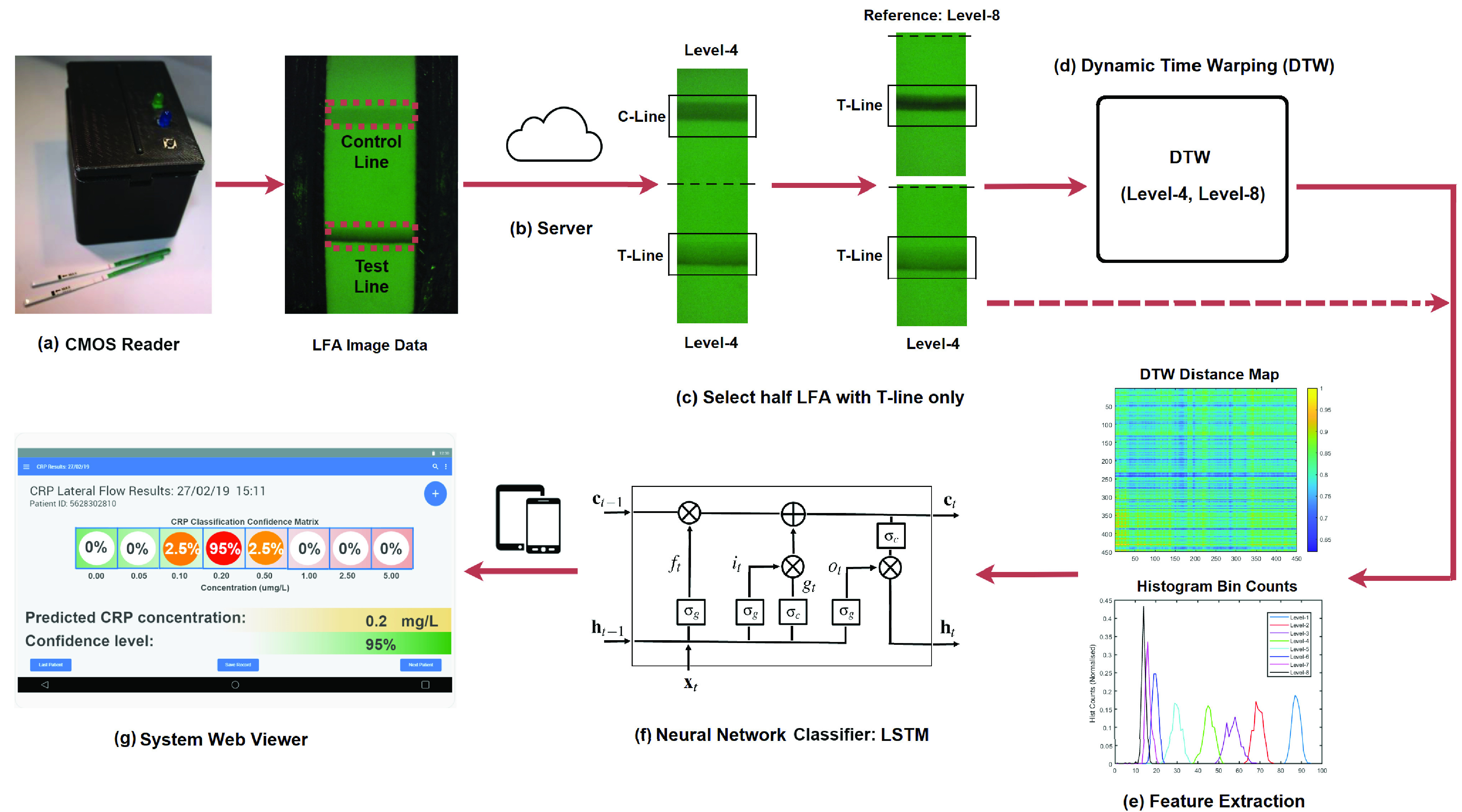
Overview of the proposed system architecture: (a) the external view of the designed CMOS reader, in which the LFA image was taken by a CMOS camera with the control line (C-Line) and test line (T-line); (b) data were transmitted to a secured internal server for data storage, analysis and results viewer; (c) half of LFA image containing the T-line only was selected for further analysis in which the concentration level-4 was used as an example; (d) DTW was applied to level-4 LFA and a reference LFA from level-8; (e) feature extraction from DTW distance map or histogram bin counts; (f) classification via the LSTM networks; (g) a web viewer user interface where the end-users can view and query the results of classification.

III. Data Acquisition

A. LFA Structure

LFA are operationally intuitive with a long shelf life and by virtue of a paper-based construction, can facilitate passive sample and reagent processing via capillary flow. Most conventional lateral flow tests use the ‘sandwich’ assay format, in which a biomolecule of interest (located in the sample) is simultaneously bound (sandwiched) between two different antibodies - one attached or conjugated to the detection label, and the other immobilised on a T-line zone on the reaction membrane. A schematic illustration of LFA is given in Fig. 2, which shows the sample pad, sample flow direction, conjugate pad, T-line, C-line and absorbent pad. The conjugate pad, containing colloidal gold, is labelled with antibodies specific to the target analyte (conjugate). When the sample is placed on the sample pad, it flows by capillary action to the conjugate pad where the target analyte can interact (bind) with these labelled conjugate antibodies. Conjugate and any conjugate-sample complexes then travel laterally along the strip. Upon reaching the T-line, any formed conjugate-sample complexes are captured and may begin to accumulate over the remainder of the assay time. Once these reach sufficient density a visual change occurs on the T-line. The qualitative indication of the presence/absence of a biomarker can be achieved through the presence/absence of a T-line. T-line label accumulation can occur in a manner proportional to biomarker concentration. The purpose of the C-line is to capture remaining colloidal gold conjugate, regardless of presence of the target analyte, therefore C-line acts as a quality control to assess whether the system is working correctly.

FIGURE 2.

The schematic illustration of the LFA structure.

B. Manufacturing and Assembly of LFA Strips

The LFA strips were manufactured by dispensing the anti-CRP antibody (1mg/ml) onto nitrocellulose membrane (Sartorius AG) at a flow rate of /cm using a front-line dispenser (Biodot, ZX1010). This line of reagent will be referred to as the T-line. A second separate and parallel C-line was dispensed exactly 5.5mm from the T-line. The C-line comprised of goat anti-mouse Immunoglobulin G (IgG) antibody (1mg/ml). Printed nitrocellulose membranes were dried at 37 1()()55(4010) 01

Eight concentrations of CRP solutions (0, 0.05, 0.1, 0.2, 0.5, 1, 2.5 and 5 mg/L) were prepared in a Phosphate-buffered saline (PBS) solution to demonstrate proof of concept of LFA. The prepared sample of CRP standard solutions ( ) were applied to the lateral flow assay with Gold-CRP-nanoparticles ( ) and running buffer ( ) as a 10 minute wet assay. A ‘sandwich’ assay was employed with the colour intensity at the T-line relating to concentration of CRP in the sample.

C. Image Acquisition Via CMOS System

Proper illumination is critical to produce precise analysis of the LFA. Since external ambient light sources can affect the image quality, the designed CMOS reader was placed in an opaque 3D printed casing to control the lighting on LFA strip. The box was constructed to be intuitive and user-friendly, which can be operated with only one push button switch installed onto the device and two external LED lights (green and blue) indicating state of data transmission (as shown in Fig. 1 (a)). The LFA strip was inserted into the small inlet near the base of the reader. Once switched on, the green LED will illuminate to indicate that the strip data was processed and sent to the cloud for analysis. Once the image acquisition was over, the green LED will turn off. However, if there were connectivity problems the blue light will turn on and stay on until a reliable and stable connection to the cloud was established.

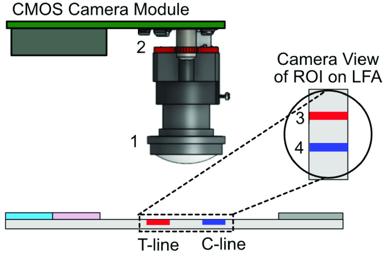
For most LFA readers, T-line and C-line alignment with the sensors is critical to avoid major discrepancies in the result. Some systems use different sensors and light sources to measure the intensity changes at the test and control line independently. Other method (such as flatbed scanner) uses a single sensor and light attached to a mechanical arm to scan the LFA strip, which increase hardware costs, power consumption and complexity of the overall system. This study used a single CMOS camera to take an image of the LFA containing both T-line and C-line areas. The inner structure of the designed CMOS reader light box is shown in Fig. 3. The CMOS camera was aligned directly above the LFA in a stationary position, removing the requirement of a mechanical arm and issue related to poor alignment with the sensor. Four green diffused Surface-Mounted LEDs with large viewing angles were positioned evenly around the CMOS camera lens to provide an even distribution of light across the testing region of the strip. Since the gold nanoparticles used in this study have a diameter of 40nm, the light of wavelength 530nm (green) was used [30] to increase the level of absorption which in turn increases the amplitude of the signal-to-noise ratio.

FIGURE 3.

Inner structure of the designed CMOS reader light box: 1) CMOS lens point downwards onto the LFA strip; 2) four green LEDs evenly distribute light onto the LFA; 3) T-line and 4) C-line on LFA strip.

Arducam’s OV5642 CMOS 5-megapixel camera module was used for image acquisition due to its low power consumption and high performance, which makes it ideal for a battery powered PoC devices. The Particle Photon WiFi development board, with a Cypress BCM43362 WiFi chip and STM32F205 120Mhz ARM Cortex M3 microcontroller, was used to send the images to the cloud as well as controlling the Arducam’s CMOS sensor timings and LED controls.

D. LFA Image Data

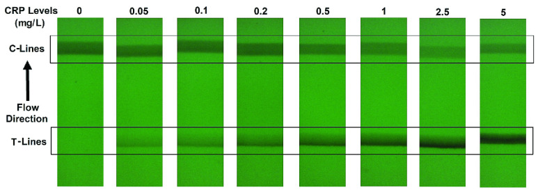
Fig. 4 gives examples of a set of LFA strip images obtained at eight hsCRP concentration levels using the designed CMOS reader system. The eight levels (in mg/L) are: 0, 0.05, 0.1, 0.2, 0.5, 1, 2.5 and 5. It can be seen that each strip contains the C-line and T-line, in which the intensity of the T-line changes according to the concentration levels. It is also noticed that the position of the T-line is not fixed in each image. For those approaches based on averaging the image intensity from T-line area (ROI), the performance can be affected by the accuracy of ROI detection. Feature based on intensity may work for simple binary classification but a more sophisticated approach is needed for detection of high-sensitivity biomarkers, especially for the LFA at low concentration level that can have a very faint T-line. The length of an LFA strip image along the sample’s flow direction is 1600 pixels, which was also considered as the time steps in this study. The width of LFA strip is 450 pixels. In this paper, the number of row of an LFA image is defined by the width of strip and the number of column is the length of LFA strip along the flow direction. Only half of LFA image containing the T-line (size pixels) was used for further analysis.

FIGURE 4.

Examples of LFA strip images at eight hsCRP concentration levels captured by the designed CMOS system.

Note that the purpose of this study was not to analyse the LFA strip at discrete or continuous time points as the assay proceeds. Instead, the LFA images were captured at a fixed time point (also known as an endpoint assay), following ‘completion’ of the lateral flow assay. The LFA image is a final snapshot of the assay containing a particular spatial phenomenon, i.e., the leading edge is stronger than the trailing edge, which also contains valuable time-dependent information that can help to enhance the classification performance.

IV. Multilevel Classification

This study developed a novel approach considering the LFA data along the sample’s flow direction as time series signals (hence no need for ROI detection), which provided a new perspective to analyse the LFA image data and explore richer information than image intensity. For classification, the LSTM networks can be directly applied to the LFA time series signals (as in our pilot study [31]) however the performance can be improved with additional features. Here, the temporal features were constructed from DTW [27] and histogram bin count. LSTM networks [29] are a special kind of RNN that are able of exhibiting dynamic behaviour and learning the long-term dependencies along a temporal sequence and have been successfully applied to speech recognition [32], language modelling [33] and ECG arrhythmia detection [34], [35]. DTW [27] developed an optimum dynamic programming (DP) based time-normalisation algorithm for spoken word recognition, which has been widely used in many applications such as to find patterns in time series [36], word recognition [37], brain signal processing [38] and motion capture [39].

A. Features Via DTW Distance Map

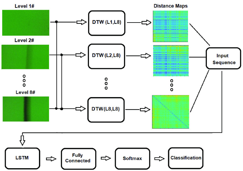
A block diagram of the framework incorporating LSTM and DTW for classification of eight hsCRP concentration levels is given in Fig. 5. Since C-line worked as a quality control, only the half of LFA image containing the T-line was selected for classification. Because LFA time series reveal the change of intensity with time steps (as in the example given in Fig. 8(a)), DTW was applied to align the LFA time series from each concentration level to one reference LFA image from level-8. The distance maps obtained from DTW capture the feature of alignment, which are arranged as the input sequences for LSTM, followed by a fully connected layer, a softmax layer and an output layer for sequence classification. Alternatively, the features can also be formed based on the histogram bin counts from the distance maps or the LFA time series (as explained in Section B), which can be used as the input sequences for LSTM.

FIGURE 5.

The block diagram for the proposed framework for multilevel hsCRP classification via incorporation of LSTM and DTW.

FIGURE 8.

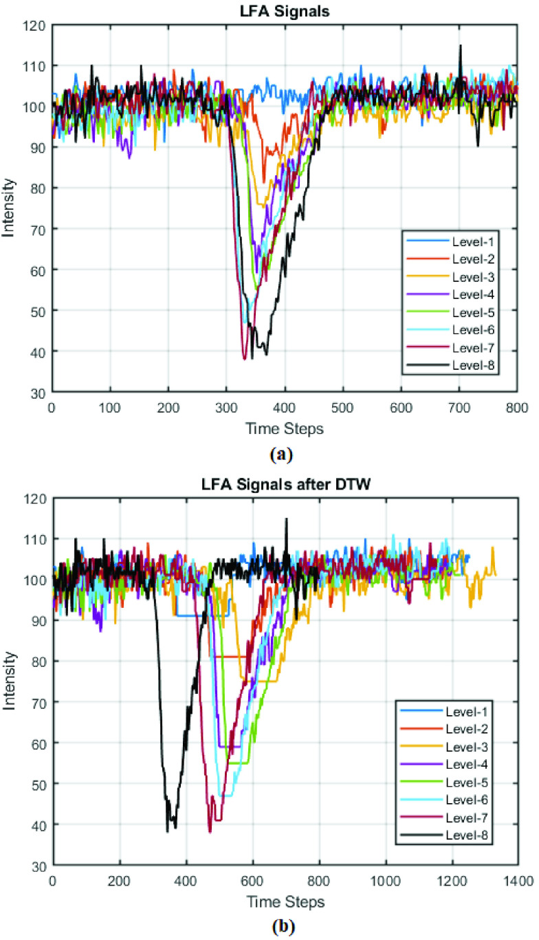
LFA time series from eight concentration levels: (a) original signals; (b) signals after DTW.

For half LFA image with size pixels, in which 450 is the width of LFA strip and 800 is the length across the strip (along the flow direction). Each row of images is considered as a time series (with 800 time-steps) since they contain the information that arises as a result of temporo-spatial interactions throughout the assay time via the gradual accumulation of label conjugate particles. To apply DTW, each row of LFA images at different concentration levels was aligned to the corresponding row in a reference LFA (from level-8), therefore, the distance map is a matrix with dimension of . One fixed LFA image from level-8 was used so that all data were compared with the same reference.

B. Features Via Histogram Bin Counts

To explore the temporal features that capture the differences across all CRP levels, the feature of histogram was investigated. After aligning eight CRP levels to the reference by DTW, each distance map was rescaled to a range of [0, 1]. Fig. 6 presents the image histogram for the rescaled distance map, which clearly shows the differences in eight CRP levels. A new feature was formed via the histogram bin counts (HBC) for each row of the rescaled distance map. The number of bin was set as 100 (hence all features have the fixed length of 100). The histogram bin counts were normalised by probability to make the sum of the bin values to be less than or equal to 1. Therefore, for each distance map (size ), the feature of HBC has a size of .

FIGURE 6.

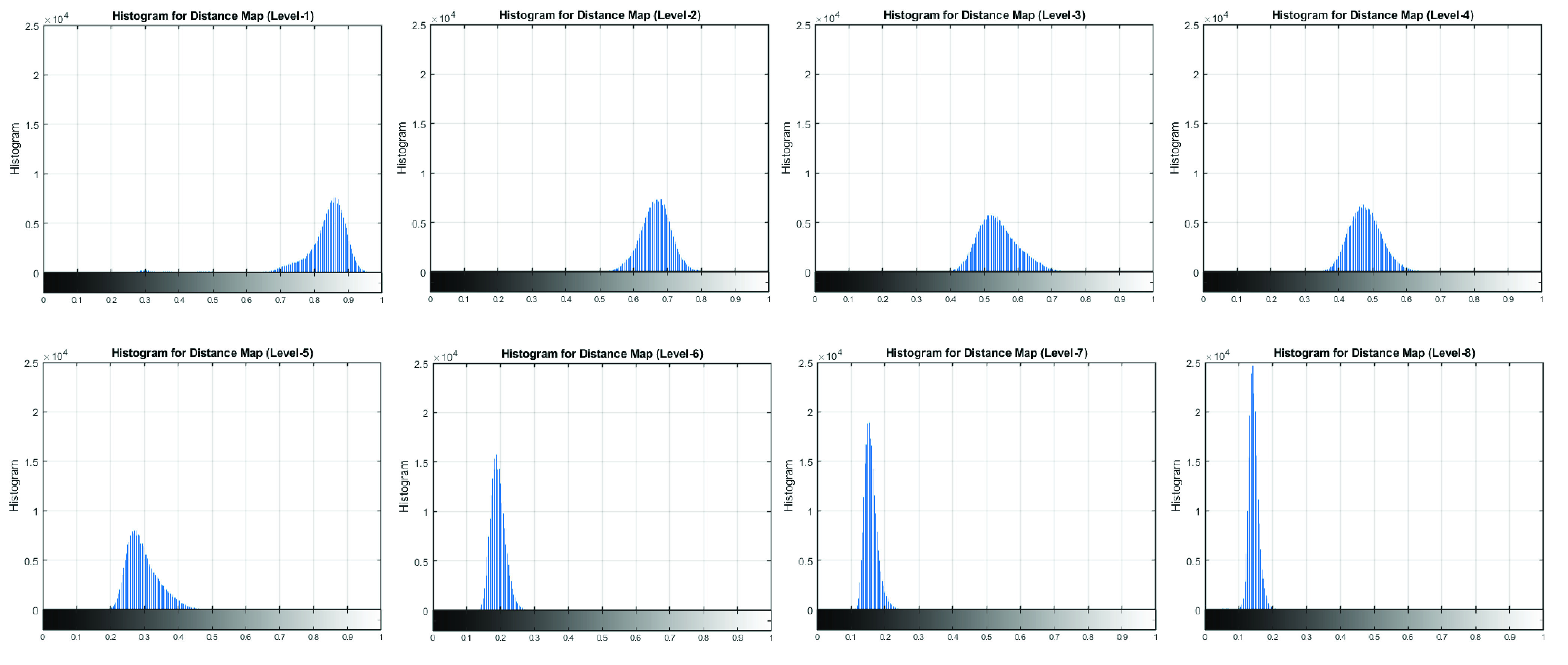
The image histogram for the distance map from DTW after aligning eight CRP levels to a reference at level-8.

The same approach was applied to obtain the HBC features from the LFA time series data (without DTW). For each level LFA (size ) the HBC feature has the same size as that from distance map ( ). The performance based on the distance map and HBC features were evaluated and compared in the experiments.

C. Arrangement for LSTM Input Sequences

It was noticed that the performance of LSTM can be affected by different feature dimensions or input sequences. Given an input sequence for LSTM sequence , which can be presented in a matrix form:

where is the feature dimension and is the feature length. For the feature based on the DTW distance map, , and for HBC features . It was noticed that by changing the feature dimension we can have different number of input sequences, such as by dividing the original features into a number of smaller-size feature sets. For example, with the maximum dimension , number of input sequence is 1; if , the number of sequences from original feature becomes 450/45 = 10, which may have impact on the performance of LSTM. In the experiment, the different combinations of and the number of sequences were investigated and performance was compared.

V. Experimental Results

In the experiments, the evaluation of designed CMOS system was carried out first followed by the classification of LFA data obtained from eight hsCRP concentration levels. Each level has 30 LFA images (hence 240 images in total). Each image (size ) contains 450 time series so the total number of time series available is . A holdout data partition was used, in which 70% were randomly selected for training and the remaining 30% for testing. The number of input sequences for training and testing under different arrangements are given in Table 1, in which the first column shows the number of feature dimensions and input sequences that can be obtained from either a distance map or the feature of HBC. The accuracy was defined as: sum(Predict = Test)/(Number of Test). The number of epochs, batch size and iteration rate for LSTM were empirically set to 30, 20 and 0.01, respectively. The distance maps were rescaled to a range of [0, 1] before being normalised by zscore and fed into the LSTM network. All numerical aspects of the experimentation were conducted using MATLAB2019b.

TABLE 1. Size of Input Sequences for Training and Testing.

(Dimension, Sequences)	Training	Testing
(10, 45)	7560	3240
(15, 30)	5040	2160
(30, 15)	2520	1080
(45, 10)	1680	720
(90, 5)	840	360

A. Performance for CMOS Reader

The performance of CMOS reader was compared to a commercial device from Lumos Diagnostic (lumosdiagnostics.com), which is a well-developed product and has been widely used in laboratories. The Lumos system is a reusable LFA reader and analyser that provides high-resolution imaging of LFA strips for qualitative and quantitative applications, however it was not designed for the purpose of this study (involving multilevel high-sensitivity biomarkers).

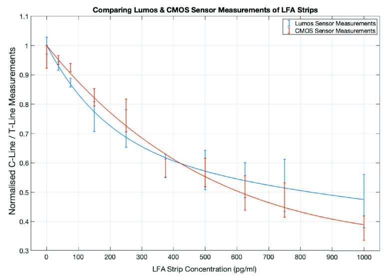
The original LFA images (RGB) were converted to the grayscale first, then manually cropped to remove unwanted sections of the image and keep the LFA strip. The change in the pixel intensity shows the change from the background of LFA to the two darker regions for T-line and C-line. The pixel values of both regions were averaged to obtain the mean intensity of the T-line and C-line regions. To mitigate the variations that might be introduced by the LFA strips and image lighting, the ratio of mean intensity from C-line and T-line was calculated, which was expected to vary for different concentration levels in biomarker sample used to produce the LFA.

Fig. 7 presents the results on the comparison of the measurements for mean intensity of Control-Test line ratio from the designed CMOS reader and Lumos system using ten commercial LFA strips (not for detection of CRP), with error bar based on the standard deviation (SD). It can be seen that the Lumos system has a steeper curve (indicating slightly more sensitive) at the lower range of concentration levels compared to the CMOS system, but the overall performance from the two systems are comparable.

FIGURE 7.

Comparison of performance from the designed CMOS reader and Lumos reader based on ten LFA strips.

B. Results from DTW

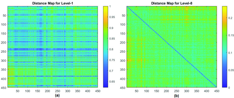
An example of one set of original LFA time series from eight hsCRP levels is shown in Fig. 8 (a), which shows that the intensity changes according to the concentration levels. Fig. 8(b) shows the results after DTW, in which the original signals from each level were aligned to the one at level-8 (which remains itself as the reference). It is noticed that the length of the signals changed as DTW stretches the original data to match the reference. The examples of two distance maps from DTW by aligning LFA level-1 and level-8 data with the reference (level-8) are given in Fig. 9 (a) and Fig. 9 (b), respectively, in which the distances are rescaled in the range of [0, 1]. It can be seen in Fig. 9 (b) that the values along the diagonal line are zeros when the rows from level-8 were aligned with themselves.

FIGURE 9.

Examples of two distance maps obtained from DTW by aligning LFA data with the reference (level-8): (a) level-1 and (b) level-8.

C. Features of HBC

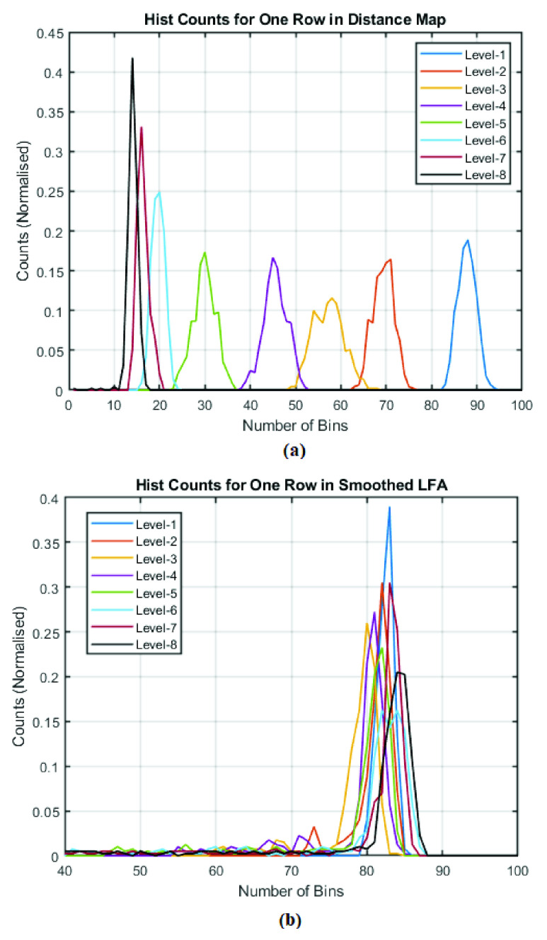
Fig. 10 presents two examples of the features from eight concentration levels based on the histogram bin counts for one row from (a) distance map and (b) LFA time series data, respectively. It can be seen that the HBC features from distance map appear to be better separated in terms of bin’s locations (along x-axis) than those obtained from LFA time series, but the latter appears to present the differences in the number of counts (in y-axis).

FIGURE 10.

The HBC features from eight concentration levels for one row in: (a) DTW distance map and (b) LFA time series data.

D. Results from Classification

The classification by the proposed method was compared to five well-known machine learning classifiers including SVM, K-Nearest Neighbours (KNN), Linear Discriminant Analysis (LDA), Decision Tree (DT) and Naive Bayes (NB). For fair comparison the same data partition was used to test all algorithms and same size of sequences as shown in Table 1. The multiclass models were trained based on the error-correcting output codes (ECOC) model [40] and the hyperparameters for each classifier were obtained via running the hyperparameter optimisation process set in Matlab.

For LSTM the performance may be affected by different settings for feature dimension and the number of hidden layers in LSTM. The experiments were carried out by changing the feature dimension as 10, 15, 30, 45 and 90 as set in Table 1. For the HBC features for LFA time series, the number of hidden layers were 10, 25, 50, 100, 150, 200, 250 and 300. The results suggest the overall good performance for all input dimensions is hidden layers 250. Similar experiments were carried for HBC features obtained from distance map, the best setting for hidden layers was 150. For the distance map, the best performance was found for hidden layer 25.

The results based on the DTW distance map, HBC features for distance map and LFA time series are given in Table 2, Table 3 and Table 4, respectively. For two features based on DTW, the results from LSTM based on distance map (Table 2) appear to perform better than those based on their HBC features (Table 3). Interestingly, the HBC features for LFA time series data (Table 4) appear to achieve the best performance. In addition, LSTM outperforms other classifiers for all three cases (with or without DTW).

TABLE 2. Classification Based on DTW Distance Map.

Accuracy (%)
Classifiers	(10,45)	(15,30)	(30,15)	(45,10)	(90,5)	Mean ± SD
SVM	86.42	87.31	87.78	87.36	87.50	87.27 ± 0.51
KNN	83.33	82.59	79.17	77.78	75.28	79.63 ± 3.35
LDA	83.33	88.15	84.81	84.86	85.83	85.40 ± 1.78
DT	78.89	76.81	70.83	73.89	71.11	74.31 ± 3.53
NB	75.96	80.74	77.5	80.69	75.83	78.14 ± 2.44
LSTM	90.15	89.35	92.59	90.83	90.28	90.73 ± 1.38

TABLE 3. Classification Based on HBC Features for DTW Distance Map.

Accuracy (%)
Classifiers	(10,45)	(15,30)	(30,15)	(45,10)	(90,5)	Mean ± SD
SVM	81.70	81.16	81.02	82.08	78.77	80.95 ± 1.29
KNN	80.96	83.75	79.81	81.53	81.67	81.54 ± 1.43
LDA	82.04	81.71	79.81	81.67	81.39	81.32 ± 0.88
DT	83.27	80.88	77.96	78.89	78.06	79.81 ± 2.26
NB	78.92	77.64	78.80	79.31	76.39	78.21 ± 1.19
LSTM	86.08	86.85	92.41	86.17	87.50	87.80 ± 2.64

TABLE 4. Classification Based on HBC Features for LFA.

Accuracy (%)
Classifiers	(10,45)	(15,30)	(30,15)	(45,10)	(90,5)	Mean ± SD
SVM	92.69	91.44	92.96	94.44	90.00	92.31 ± 1.67
KNN	87.44	84.21	89.54	86.11	75.28	84.52 ± 5.52
LDA	92.59	93.47	93.06	92.78	91.11	92.60 ± 0.90
DT	86.54	84.77	85.28	82.78	83.89	84.65 ± 1.42
NB	89.14	88.19	80.19	85.97	80.56	84.81 ±4.21
LSTM	95.80	94.81	94.17	92.92	93.06	94.15 ± 1.21

We further compared the performance at each concentration level of an LSTM model and three top ML algorithms (ranked by their average accuracy) based on three features in Table 2, Table 3 and Table 4, in which the feature dimension was 30. The results are further presented in Fig. 11 in confusion matrices. It can be seen that for all classifiers the HBC features for LFA time series lead to the highest accuracy, the higher errors are found for classifying level-5, 6, 7 and 8. For HBC features for LFA, the three ML classifiers performed better than the LSTM model at level-5 and level-6 and LDA appears to be better than SVM and KNN. For the Distance Maps and their HBC features, the three ML classifiers performed better than LSTM at level-2 and KNN has higher accuracy than SVM and LDA. The overall performance for classification suggest the ability to output of the concentration of the target analyte with a high level of accuracy by the proposed approach via applying LSTM to different features obtained from LFA time series and DTW.

FIGURE 11.

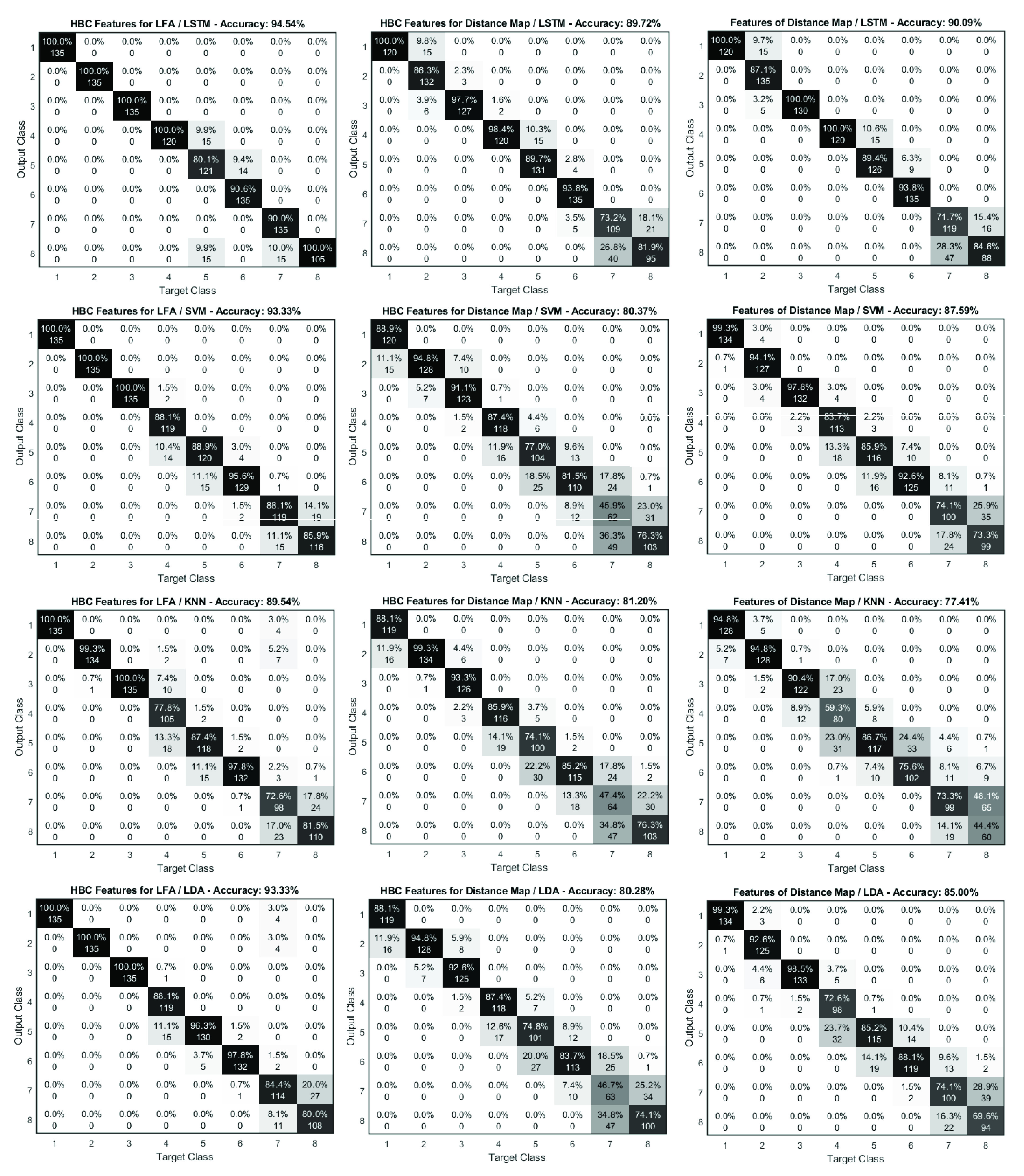
Comparison of confusion matrix from classification based on LSTM, SVM, KNN and LDA using features of distance map, HBC features for distance map and HBC features for LFA time series.

E. Comparison with ROI-Based Approach

The proposed method has two advantages over the ROI-based approach. First, ROI detection can be difficult when the sample’s concentration level is very low and an advanced method is needed as reported in some studies [23], [24]. Second, the proposed method treats the signal along the sample’s flow direction (each row of the image) as a time series, which captures the temporal information that is usually ignored by averaging the intensity within the ROI and therefore can potentially improve the classification performance.

1). ROI Detection

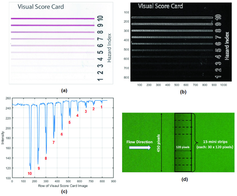
To demonstrate the impact of T-line intensity on ROI detection, a visual score card was used as an example in Fig. 12(a), which includes the T-lines at 10 intensity levels. Fig. 12(b) presents the detected T-line area using the traditional Sobel edge detection technique. It can be seen that the regions with intensity lower than level-3 were hard to detect. Fig. 12(c) plots the intensity values taken from the column in visual score card image (Fig. 12(a)). The x-axis is the number of rows of the image and y-axis is the intensity, which shows the intensity values being captured at all 10 levels (as marked in red).

FIGURE 12.

(a) A visual score card showing the T-lines with 10 intensity levels; (b) T-line regions detected by Sobel edge detection; (c) plot of intensity values at the column of visual score card; (d) define the ROI from half of LFA image containing T-line.

2). Classification

The ROI-based approach was applied to the same LFA image based on eight hsCRP levels. To extract the T-line area, firstly, the minimum intensity value was found from the half of the LFA image containing the T-line. The ROI was defined by a rectangular region from the point of minimum value plus 120 pixels along the flow direction (as illustrated in Fig. 12(d)). (Here the ROI width of 120 pixels was determined empirically, which could be wider to simplify the process). Each image was divided into 15 mini strips each with dimensions of pixels. The intensity along the flow direction was averaged so each mini strip provides the mean of intensity ( ), which were used for classification.

A holdout data partition was used, in which 70% of available data were randomly selected for training and the remaining 30% for testing. For comparison, the proposed methods were also applied to the raw LFA time series based on dimension 30 and sequence 15. The number of feature vectors is 2520 for training and 1080 for testing. The results based on accuracy are provided in Table 5, which show that using the LFA time series achieved better performance than the mean from ROI. In addition, the results from LFA time series are not as good as those (with dimension 30 and sequence 15) in Table 2, Table 3 and Table 4, because further temporal feature extraction (by either DTW or HBC) helps to improve the classification performance.

TABLE 5. Classification Accuracy (%) by the ROI-Based and Proposed Method.

Classifiers	Mean from ROI	LFA Time Series
SVM	50.46	58.61
KNN	48.24	49.17
LDA	50.46	53.33
DT	45.28	50.28
NB	48.52	62.60
LSTM	–	73.33

F. Application to LFA Images from Human Plasma

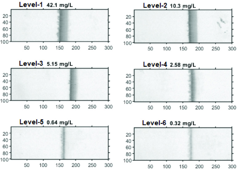
To demonstrate the application of the proposed method to actual human samples, the LFA images for human plasma were assembled based on dilution of the certified reference material ERM-DA474/IFCC, which has been used as a reference material for CRP since 2012 [41]. The original sample with concentration 42.1mg/L was diluted to produce six concentration levels (in mg/L): 42.1, 10.3, 5.15, 2.58, 0.64 and 0.32. Lumos reader was used to capture the LFA images since the CMOS reader designed in this study (for hsCRP) was not optimised for the plasma samples.

Fig. 13 shows one set of LFA images with six concentration levels obtained from the Lumos reader, in which the T-line area was cropped to a size of pixels. It can be seen that the intensity of T-line area changes according to the concentration levels. Two sets of LFA images were acquired by the Lumos initially. To increase the number of data points for classification, each image was split into half (size pixels) first, then flipped vertically and horizontally, finally produced 12 image sets in total for classification. Flipping the image will not change the mean or variance of time series, such as flipping LFA image vertically only rearranges the order the time series. Flipping LFA image horizontally does change the pattern of LFA time series since it inverses the flow direction of time series, which can affect the performance if one uses the raw LFA time series or DTW for classification, but should not affect the HBC features for LFA time series (since it is based on the histogram bin counts). For comparison, the mean from the ROI, raw LFA time series and the HBC features for time series were used for classification.

FIGURE 13.

The LFA images based on diluting the human plasma in six concentration levels.

The number of final plasma LFA image sets used for classification were 12, in which 8 sets were randomly selected for training and the rest of the 4 sets were used for testing. The size of the image (after splitting the original image into half) is . The feature dimension was set as 10 so each image contains 5 sequences (or mini strip images). For ROI-based approach, since size of each mini strip is relatively small ( pixels), we directly used it as ROI and the mean of intensity along the flow direction was calculated and each mini strip has a feature vector ( ). The total number for training and testing was 240 and 120, respectively. Since the data is too small to train LSTM network, only five traditional ML classifiers were used in this experiment.

The results based on the mean from ROI, LFA time series and HBC features for time series using five classifiers are provided in Table 6. It can be seen that the performance by the proposed method using LFA time series and HBC features are better the mean of the ROI. As expected, higher accuracy was achieved by HBC features comparing to using the LFA time series. The performance based on the LFA time series can be affected due to flipping the image horizontally which changed the flow direction of the time series. Despite this, the overall performance from LFA time series is still better than that from the mean of ROI.

TABLE 6. Comparison of Classification Accuracy (%).

Classifiers	Mean from ROI	LFA Time Series	HBC for LFA Time Series
SVM	60.0	59.2	80.0
KNN	60.0	70.8	85.8
LDA	45.0	63.3	95.8
DT	33.3	55.0	60.8
NB	43.3	65.8	48.3
Average	48.3	62.0	74.1

The confusion matrices for the top three classifiers are provided in Fig. 14. Overall, HBC features for LFA from LDA appear to perform well at all levels. The errors from the ROI-based approach are found at level-2, 3 and 4. But for level-5 and level-6, the SVM and KNN based on the mean of ROI appears to work better than the proposed methods. Note the performance of classification is not the focus here, instead, the purpose of this experiment was to demonstrate the feasibility of the proposed method for actual human samples. The overall results suggest the possible potential of the proposed system for real world applications.

FIGURE 14.

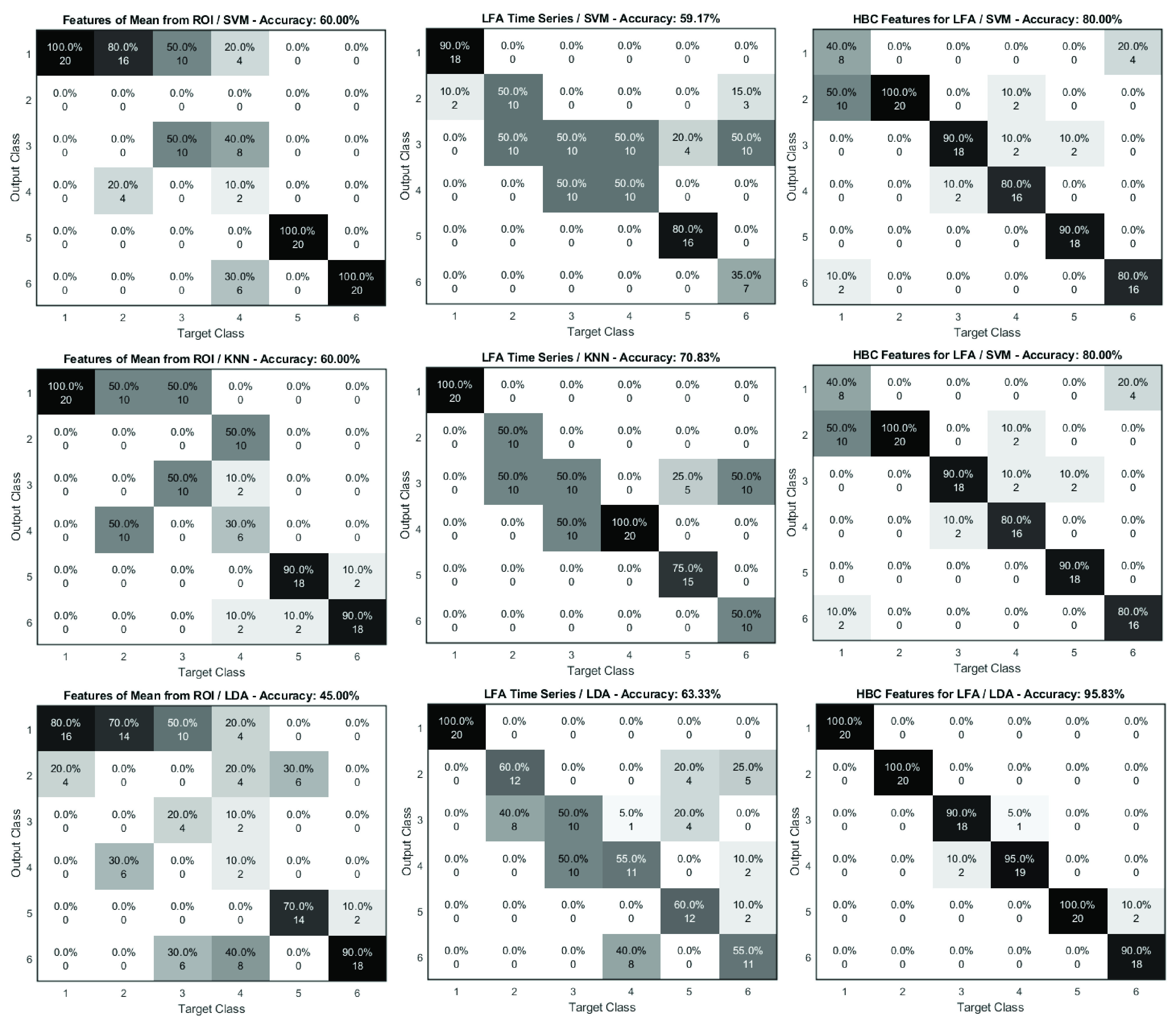
Comparison of confusion matrix from classification based on SVM, KNN and LDA based on different features: mean from ROI, LFA time series and their HBC features.

VI. Discussion

This study developed an easy-to-use LFA reader system, which can provide the user with a more in-depth quantitative analysis for LFA images than the conventional approaches. The proposed approach for considering the LFA image data along the sample’s flow direction as a time series of signals provided a new perspective to analyse the image data. By capturing the temporal information from an image provides us with more opportunity for data exploration which will potentially help to improve the system performance in general. The presented idea can be useful for various image analysis applications that involve the data containing both spatial and temporal information.

An end-to-end system has been developed and implemented whereby a light-box was constructed to control environmental variables with an intuitive design allowing the user to obtain the LFA image data at the press of a single button. The data can be sent to a remote server via IoT device, where the image data can be analysed and results are displayed on a web application.

Unlike conventional semi-quantitative analysis methods, the proposed approach encourages system calibration (model training) using samples that are more reflective of those encountered in real-world PoC system. This opens the door to accurate, non-subjective biomarker analysis that can cope with the challenge of the artefacts caused by use of heterogeneous samples and subsequential false positives/negatives against a set threshold. The use of a back-end system can ensure that the appropriate calibration in case with variability in the sample matrix may lead to the necessity of recalibration of readers.

CRP is a good predictor of heart disease, there’s a high correlation between high CRP levels and the chances of having a heart attack or cardiovascular problems. As reported in [12], of the 12 biomarkers tested, the hsCRP measurement resulted as the strongest univariate predictor for cardiovascular events. Some studies [13] suggested using hsCRP as a discriminatory tool through division of three or even five categories ranging from < 1mg/l to >5mg/l. Another study [42] shows that dividing hsCRP levels into five categories (< 0.5mg/l, 0.5-1mg/l, 1-3mg/l, 3-5mg/l, and >5mg/l) could provide further discrimination. Therefore, to investigate the capability of analysis in the CRP range associate to CVD risk assessment, we analysed the hsCRP at eight concentration levels in a range of 0-5mg/L, which were aligned with clinically actionable categories for early risk assessment of CVD. The developed method needs to be highly sensitive, which is crucial due to the minor variance at those low CRP levels that will importantly determine cardiovascular risk. The positive outcomes for classification of multilevel hsCRP in this study demonstrated the real-world applicability for the proposed approaches.

As a proof of concept, the major work in this study used CRP as a model assay in a buffer system. To demonstrate the proposed method works on actual samples of blood or plasma, the additional LFA images from human plasma were assembled by using the certified CRP reference material (as in Fig. 13). We analysed LFA from plasma as the sample matrix and results for classification are given in Table 6. The performance could be limited due to only small plasma image data was available for the experiment. Due to the complexity of real samples, more consideration will be needed when apply the proposed methods to real-world problems. (1) In term of data generation, within a biological context, blood and plasma matrix compositions are often complex and contain many small compounds of varied character, proteins, and other small to large cellular components. These many components in biological matrices can influence the result of an analysis; (2) In terms of data acquisition, the design of CMOS reader may need to be adaptive for LFA with different targets (or antibodies); (3) For data analysis, the LFA images from real samples may contain the stains (as noticed in Fig.13 for plasma sample level-2, which can simply be dust or contaminants). Also as pointed out in [23], when the user adds the sample to LFA device some interference noises can be inevitable on the strip due to variations in sample matrix (e.g. urine, blood, serum) or the actual differences in the constituents of the individual sample. The stains (or noises) on LFA image can affect the analysis performance therefore additional prepossessing (either manual or automatic) are needed to detect and ‘clean’ such artefacts before further image analysis.

The limitation of the study includes the following aspects. (1) Despite the ability of antibodies to detect target antigens in complex matrices, immunoassays have their limitations. Different LFA may be difficult to implement with the existing system due to different affinities of antibodies. This would mean that each LFA for different targets (or antibodies) would have to be optimised and validated each time via a calibration curve which is standard practice where quantitative results are required. For hardware settings, to achieve the best performance, the design of a CMOS reader may need to be adapted and optimised for LFA with different targets. Current setup using the green LEDs was designed specifically for LFA (hsCRP) used in the paper as to maximise the absorption of light photons by the gold nanoparticles at 530nm. The same setup (with green lights) can still be used with other LFA strips not using gold nanoparticles (such as in our study based on LFA with NT-proBNP for heart failure [43]), but may result in some reduced sensitivity. Alternatively, the LEDs can be changed from green to white light source to have uniform lightning throughout the visible spectrum, allowing the system to be used for multiple strips, which is currently under development. (2) CRP is a general nonspecific marker of inflammation, it is useful in helping predict the risk of heart disease. However, analysing CRP on its own may not be totally beneficial. Instead analysing CRP along with other biomarkers (e.g. cholesterol) may give a better indication of the risk of cardiovascular issues and help to evaluate disease progression and prognosis in those who already have cardiovascular disease. (3) The overall results from hsCRP suggest that LSTM has the advantages over traditional ML classifiers. For small data sets (for plasma samples), LSTM’s performance was not stable (so not reported) since it needs large data to train the network, but the traditional ML classifiers with feature extraction performed better than LSTM. (4) The performance based on human plasma samples could be limited due to only small plasma image data was available, because this study was conducted during COVID-19 pandemic and it was difficult to collect the human blood or plasma samples. A full clinical trial using human blood or plasma to validate the system will be considered in the next stage of this research. Nevertheless, the experimental results have demonstrated the applicability of the proposed method to real human samples.

Future development may consider to improve the image quality by having uniform controlled lightening in the casing, using a higher resolution CMOS camera and suitable lens to better focus on the ROI of the LFA. A fully integrated analysis system may also include a quality control to ensure the assay has performed correctly via detection of C-line before analysis of T-line. Future work may also include the image quality check during data acquisition stage, which helps to identify and exclude the images containing the stains on LFA strips thereby improve the quality of features. Ultimately, the system will be embedded into a chip (Lab-on-a-Chip), where the results can be displayed on the lightbox without transmitting to and from the cloud. More future work may conduct analysis on wet strips, variation of LFA strips, together with exploring other options of neural networks.

VII. Conclusion

This study developed a portable LFA analyser device containing a CMOS camera integrated with custom illumination and optics, in which the device was integrated with a back-end server system for data aggregation, analysis and results displaying. The development for LFA data generation, image data capture and data analysis were described in detail. A novel classification framework is presented, which enhances the detection of multilevel hsCRP biomarker in LFA testing via considering LFA image as the time series, which provides a new perspective for LFA analysis and potential to capture valuable temporal information richer than image intensity alone. Features based on DTW and HBC were investigated with different arrangement for input sequences for LSTM. The outcomes based on multilevel hsCRP with concentration below 5 mg/L are encouraging, which suggest the potential of the proposed system for early risk assessment of CVD. Furthermore, the results based on human plasma suggest the feasibility of the proposed system for real-world applications.

Funding Statement

This work is part of the Eastern Corridor Medical Engineering Centre (ECME) project and funded by the European Union (EU) European Territorial Cooperation (INTERREG VA) Cross-border Programme (2014-2020), managed by the Special EU Programmes Body (SEUPB) (Grant ID: IVA5034).

References

- [1].Cardiovascular Diseases (CVDs), World Health Org., Geneva, Switzerland, May 2017. [Google Scholar]
- [2].Boxer J., Weddell S., Broomhead D., Hogg C., and Johnson S., “Home pregnancy tests in the hands of the intended user,” J. Immunoassay Immunochem., vol. 40, no. 6, pp. 642–652, Nov. 2019. [DOI] [PubMed] [Google Scholar]
- [3].Valanis B. G. and Perlman C. S., “Home pregnancy testing kits: Prevalence of use, false-negative rates, and compliance with instructions,” Amer. J. Public Health, vol. 72, no. 9, pp. 1034–1036, Sep. 1982. [DOI] [PMC free article] [PubMed] [Google Scholar]
- [4].Peck R. B.et al. , “What should the ideal HIV self-test look like? A usability study of test prototypes in unsupervised HIV self-testing in Kenya, Malawi, and South Africa,” AIDS Behav., vol. 18, no. S4, pp. 422–432, Jul. 2014. [DOI] [PubMed] [Google Scholar]
- [5].Ndlovu Z.et al. , “Diagnostic performance and usability of the VISITECT CD4 semi-quantitative test for advanced HIV disease screening,” PLoS ONE, vol. 15, no. 4, Apr. 2020, Art. no. e0230453. [DOI] [PMC free article] [PubMed] [Google Scholar]
- [6].Rodriguez N. M., Linnes J. C., Fan A., Ellenson C. K., Pollock N. R., and Klapperich C. M., “Paper-based RNA extraction, in situ isothermal amplification, and lateral flow detection for low-cost, rapid diagnosis of influenza A (H1N1) from clinical specimens,” Anal. Chem., vol. 87, no. 15, pp. 7872–7879, Aug. 2015. [DOI] [PMC free article] [PubMed] [Google Scholar]
- [7].Atchison C.et al. , “Usability and acceptability of home-based self-testing for severe acute respiratory syndrome coronavirus 2 (SARS-CoV-2) antibodies for population surveillance,” Clin. Infectious Diseases, vol. 72, no. 9, pp. e384–e393, May 2021. [DOI] [PMC free article] [PubMed] [Google Scholar]
- [8].Pollán M.et al. , “Prevalence of SARS-CoV-2 in Spain (ENE-COVID): A nationwide, population-based seroepidemiological study,” Lancet, vol. 396, no. 10250, pp. 535–544, 2020. [DOI] [PMC free article] [PubMed] [Google Scholar]
- [9].Jing M.et al. , “User experience analysis of AbC-19 rapid test via lateral flow immunoassays for self-administrated SARS-CoV-2 antibody testing,” Sci. Rep., vol. 11, no. 1, pp. 1–13, Dec. 2021. [DOI] [PMC free article] [PubMed] [Google Scholar]
- [10].Robertson L. J.et al. , “Evaluation of the IgG antibody response to SARS CoV-2 infection and performance of a lateral flow immunoassay: Cross-sectional and longitudinal analysis over 11 months,” BMJ Open, vol. 11, no. 6, Jun. 2021, Art. no. e048142. [DOI] [PMC free article] [PubMed] [Google Scholar]
- [11].Ridker P. M., “Clinical application of C-reactive protein for cardiovascular disease detection and prevention,” Circulation, vol. 107, no. 3, pp. 363–369, Jan. 2003. [DOI] [PubMed] [Google Scholar]
- [12].Ridker P. M., Hennekens C. H., Buring J. E., and Rifai N., “C-reactive protein and other markers of inflammation in the prediction of cardiovascular disease in women,” New England J. Med., vol. 342, no. 12, pp. 836–843, Mar. 2000. [DOI] [PubMed] [Google Scholar]
- [13].Musunuru K.et al. , “The use of high-sensitivity assays for C-reactive protein in clinical practice,” Nature Rev. Cardiol., vol. 5, no. 10, p. 621, 2008. [DOI] [PMC free article] [PubMed] [Google Scholar]
- [14].Quesada-González D. and Merkoçi A., “Nanoparticle-based lateral flow biosensors,” Biosensors Bioelectron., vol. 73, pp. 47–63, Nov. 2015. [DOI] [PubMed] [Google Scholar]
- [15].Eltzov E., Guttel S., Kei A. L. Y., Sinawang P. D., Ionescu R. E., and Marks R. S., “Lateral flow immunoassays—From paper strip to smartphone technology,” Electroanalysis, vol. 27, no. 9, pp. 2116–2130, Sep. 2015. [Google Scholar]
- [16].Zangheri M.et al. , “A simple and compact smartphone accessory for quantitative chemiluminescence-based lateral flow immunoassay for salivary cortisol detection,” Biosensors Bioelectron., vol. 64, pp. 63–68, Feb. 2015. [DOI] [PubMed] [Google Scholar]
- [17].Pilavaki E., Valente V., and Demosthenous A., “CMOS image sensor for lateral flow immunoassay readers,” IEEE Trans. Circuits Syst. II, Exp. Briefs, vol. 65, no. 10, pp. 1405–1409, Oct. 2018. [Google Scholar]
- [18].Mak W. C., Beni V., and Turner A. P. F., “Lateral-flow technology: From visual to instrumental,” TrAC Trends Anal. Chem., vol. 79, pp. 297–305, May 2016. [Google Scholar]
- [19].Mudanyali O., Dimitrov S., Sikora U., Padmanabhan S., Navruz I., and Ozcan A. A., “Integrated rapid-diagnostic-test reader platform on a cellphone,” Lab Chip, vol. 12, no. 15, pp. 2678–2686, 2012. [DOI] [PMC free article] [PubMed] [Google Scholar]
- [20].Ghallab Y. H. and Yehea I., CMOS Circuits and Systems for Lab-on-a-Chip Applications. London, U.K.: Intech Open, 2016, p. 17. [Google Scholar]
- [21].Torres J. L. and Ridker P. M., “High sensitivity C-reactive protein in clinical practice,” Amer. Heart Hospital J., vol. 1, no. 3, pp. 207–211, Jul. 2003. [DOI] [PubMed] [Google Scholar]
- [22].Quesada-González D. and Merkoçi A., “Mobile phone-based biosensing: An emerging `diagnostic and communication' technology,” Biosensors Bioelectron., vol. 92, pp. 549–562, Jun. 2017. [DOI] [PubMed] [Google Scholar]
- [23].Zeng N.et al. , “Image-based quantitative analysis of gold immunochromatographic strip via cellular neural network approach,” IEEE Trans. Med. Imag., vol. 33, no. 5, pp. 1129–1136, May 2014. [DOI] [PubMed] [Google Scholar]
- [24].Zeng N., Wang Z., Zhang H., Liu W., and Alsaadi F. E., “Deep belief networks for quantitative analysis of a gold immunochromatographic strip,” Cognit. Comput., vol. 8, no. 4, pp. 684–692, 2016. [Google Scholar]
- [25].Carrio A., Sampedro C., Sanchez-Lopez J., Pimienta M., and Campoy P., “Automated low-cost smartphone-based lateral flow saliva test reader for drugs-of-abuse detection,” Sensors, vol. 15, no. 11, pp. 29569–29593, Nov. 2015. [DOI] [PMC free article] [PubMed] [Google Scholar]
- [26].Jing M.et al. , “Enhance categorisation of multilevel high-sensitivity cardiovascular biomarkers from lateral flow immunoassay images via neural networks and dynamic time warping,” in Proc. IEEE Int. Conf. Image Process. (ICIP), Oct. 2020, pp. 365–369. [Google Scholar]
- [27].Sakoe H. and Chiba S., “Dynamic programming algorithm optimization for spoken word recognition,” IEEE Trans. Acoust., Speech, Signal Process., vol. ASSP-26, no. 1, pp. 43–49, Feb. 1978. [Google Scholar]
- [28].Navarro-Paredes C., Jing M., Finlay D., and McLaughlin J., “P8 big data platform for cardiovascular healthcare data storage and data viewer,” Heart, vol. 105, no. 4, p. A8, 2019. [Google Scholar]
- [29].Hochreiter S. and Schmidhuber J., “Long short-term memory,” Neural Comput., vol. 9, no. 8, pp. 1735–1780, 1997. [DOI] [PubMed] [Google Scholar]
- [30].Link S. and Mostafa El-sayed A., “Size and temperature dependence of the plasmon absorption of colloidal gold nanoparticles,” J. Phys. Chem. B, vol. 103, pp. 103–4212, May 1999. [Google Scholar]
- [31].Jing M.et al. , “Detection and categorisation of multilevel high-sensitivity cardiovascular biomarkers from lateral flow immunoassay images via recurrent neural networks,” in Proc. 13th Int. Joint Conf. Biomed. Eng. Syst. Technol., 2020, pp. 177–183. [Google Scholar]
- [32].Fernández S., Graves A., and Schmidhuber J., “An application of recurrent neural networks to discriminative keyword spotting,” in Proc. Int. Conf. Artif. Neural Netw. Porto, Portugal: Springer, 2007, pp. 220–229. [Google Scholar]
- [33].Jozefowicz R., Vinyals O., Schuster M., Shazeer N., and Wu Y., “Exploring the limits of language modeling,” 2016, arXiv:1602.02410.
- [34].Picon A.et al. , “Mixed convolutional and long short-term memory network for the detection of lethal ventricular arrhythmia,” PLoS ONE, vol. 14, no. 5, May 2019, Art. no. e0216756. [DOI] [PMC free article] [PubMed] [Google Scholar]
- [35].Xiong Z., Nash M. P., Cheng E., Fedorov V. V., Stiles M. K., and Zhao J., “ECG signal classification for the detection of cardiac arrhythmias using a convolutional recurrent neural network,” Physiol. Meas., vol. 39, no. 9, Sep. 2018, Art. no. 094006. [DOI] [PMC free article] [PubMed] [Google Scholar]
- [36].Berndt D. J. and Clifford J., “Using dynamic time warping to find patterns in time series,” in Proc. KDD Workshop, Seattle, WA, USA, vol. 10, 1994, pp. 359–370. [Google Scholar]
- [37].Paliwal K. K., Agarwal A., and Sinha S. S., “A modification over Sakoe and Chiba’s dynamic time warping algorithm for isolated word recognition,” Signal Process., vol. 4, no. 4, pp. 329–333, Jul. 1982. [Google Scholar]
- [38].Gupta L., Molfese D. L., Tammana R., and Simos P. G., “Nonlinear alignment and averaging for estimating the evoked potential,” IEEE Trans. Biomed. Eng., vol. 43, no. 4, pp. 348–356, Apr. 1996. [DOI] [PubMed] [Google Scholar]
- [39].Olsen N. L., Markussen B., and Raket L. L., “Simultaneous inference for misaligned multivariate functional data,” J. Roy. Stat. Soc., C Appl. Statist., vol. 67, no. 5, pp. 1147–1176, Nov. 2018. [Google Scholar]
- [40].Dietterich T. G. and Bakiri G., “Solving multiclass learning problems via error-correcting output codes,” J. Artif. Intell. Res., vol. 2, pp. 263–286, Jan. 1994. [Google Scholar]
- [41].Wu C.et al. , “Application of commutable ERM-DA474/IFCC for harmonization of C-reactive protein measurement using five analytical assays,” Clin. Lab., vol. 63, no. 11, pp. 1883–1888, 2017. [DOI] [PubMed] [Google Scholar]
- [42].Albert M. A., Glynn R. J., Buring J., and Ridker P. M., “C-reactive protein levels among women of various ethnic groups living in the United States (from the women’s health study),” Amer. J. Cardiol., vol. 93, no. 10, pp. 1238–1242, May 2004. [DOI] [PubMed] [Google Scholar]
- [43].Navarro C.et al. , “A point-of-care measurement of NT-proBNP for heart failure patients,” IEEE Access, vol. 8, pp. 138973–138983, 2020. [Google Scholar]