A multi-task deep-learning method for predicting membrane associations and secondary structures of proteins

Abstract

Prediction of residue-level structural attributes and protein-level structural classes helps model protein tertiary structure and understand protein function. Existing methods are either specialized to only one class of proteins or predict one specific type of residue-level attribute. In this work, we develop a new deep-learning method, named Membrane Association and Secondary Structure Predictor (MASSP), for accurately predicting both residue-level structural attributes (secondary structure, location, orientation, and topology) and protein-level structural classes (bitopic, α-helical, β-barrel, and soluble). MASSP integrates a multi-layer 2D convolutional neural network (2D-CNN) with a long short-term memory (LSTM) neural network into a multi-tasking framework. Our comparison shows that MASSP performs equally well or better than state-of-the-art methods for predicting residue-level secondary structures, boundaries of transmembrane segments, and topology. Furthermore, it achieves outstanding accuracy in predicting protein-level structural classes. MASSP automatically distinguishes the structural classes of input sequences and identifies transmembrane segments and topologies if present, making it broadly applicable to different classes of proteins. In summary, MASSP’s good performance and broad applicability make it well suited for annotating residue-level attributes and protein-level structural classes at the proteome scale.

Graphical Abstract

Introduction

Protein structures are essential to understanding protein function, unraveling disease mechanisms, and the design of novel therapeutic molecules. While innovations in experimental techniques continue to help determine new structures at a rapid pace, determining the structures of all proteins by experimental techniques remains impractical. Thus, computational prediction of protein tertiary structures from amino acid sequences continues to be an area of active research¹. While exciting progress was made in the past few years, especially in the 14^th Critical Assessment of Techniques for Protein Structure Prediction (CASP14)², protein tertiary structure prediction is still a challenging problem for many proteins^2–4.

Accurate prediction of secondary structures provides useful information for predicting protein tertiary structures. Over the past decades, a plethora of methods were developed for secondary structure prediction^5,6. Some of the first methods relied on statistical propensities of amino acids to form particular structures⁷, simple nearest-neighbor algorithms that involve finding short sequences of known structure that closely match stretches of the query sequence⁸, or explicit modeling of the contribution that neighboring residues make to the probability of a given structure state⁹. The accuracy of these methods hovered under 70% for the so-called Q3, a three-state prediction that classifies amino acids in likely helix (H), strand (extended, E), or coil (C) states. More accurate methods, better than 70% in Q3, were developed that use machine-learning-based models¹⁰. The machine-learning models powering these methods are often artificial neural networks^11–17 that take sequence profiles generated from multiple sequence alignments as input^11,12 or couple sequence profiles with nonlocal interactions from predicted tertiary structures to boost the accuracy of secondary structure prediction¹⁷. Recently, motivated by unprecedented performance of deep neural networks in computer vision problems¹⁸, deeper neural network architectures, such as convolutional neural networks (CNNs) and recurrent neural networks were applied to protein secondary structure prediction with accuracy improving to above 80% in Q3^6,19–21.

For transmembrane proteins (TMPs), an additional essential component of predicting the tertiary structure is to first locate all the TM segments and the orientation of the protein with respect to the membrane. These tasks are collectively known as “topology prediction”. Several algorithms have been developed over the past decades for predicting the topology of α-helical TMPs (TM-alpha) or β-barrel TMPs (TM-beta)^22,23. The earliest method of Kyte and Doolittle²⁴ for TM helix (TMH) prediction computes simple “hydropathy plots” to identify probable TMHs. While this method is conceptually simple and easy to implement, it can neither predict the “inside-outside phasing” of the helices relative to the cytoplasm, i.e. topology, nor the location of TM strands in TM-beta proteins. By combining hydropathy analysis and the “positive-inside rule”, the observation that positively charged residues are more abundant in cytoplasmic as compared to periplasmic regions of bacterial inner membrane proteins²⁵, a method dubbed TOP-PRED was developed for predicting TMHs and their topologies²⁶. While TOP-PRED identified all 135 TMHs in the 24 proteins tested with only one overprediction and correctly predicted the topology of 22 proteins, no results were reported as to how accurate TOP-PRED can locate the boundaries (N- and C- terminal ends) of TMHs. Aimed at predicting both the boundaries and topology of TMHs, the PHDhtm method, whose driving predictor is a two-level neural network system trained on 69 transmembrane proteins, was developed^27,28. TMHMM and HMMTOP²⁹ are the first methods to model membrane topology of IMPs with hidden Markov models. For transmembrane segment detection, MEMSAT3³⁰, OCTOPUS³¹ (for TM‐alpha proteins), BOCTOPUS2³² and PRED-TMBB2³³ (for TM‐beta proteins) are classic methods. Recent innovations in deep learning also enabled the development of more sophisticated methods, such as TMP-SS³⁴ and DMCTOP³⁵, for membrane segment detection and topology prediction.

While these existing methods have been widely used, they are either specialized on one class of proteins or developed to predict one specific type of residue-level attributes. In the current work, we leverage recent advances in deep neural network (DNN) architectures to develop a novel method, Membrane Association and Secondary Structure Prediction (MASSP), that simultaneously predicts residue-level structural attributes (secondary structure, location, orientation, and topology) and protein-level structural classes (bitopic, TM-alpha, TM-beta, and soluble). This is achieved by integrating a multi-layer 2D-CNN with a LSTM neural network into a multi-tasking framework. We extensively compare MASSP with several classic and state-of-the-art methods and show that MASSP performs equally well or better for predicting residue-level attributes. Furthermore, MASSP achieves high accuracy in predicting protein-level structural classes and is broadly applicable to different classes of proteins. The preliminary version of this method was successfully adopted in two previous studies for de novo tertiary structure prediction of TM-alpha proteins^36,37. In this manuscript, we describe the method in detail, demonstrate its broad applicability, and discuss aspects of its improved performance compared to some of the most popular methods in the field.

Methods

Datasets

The sets of bitopic, TM-alpha, and TM-beta proteins were all obtained from the OPM database³⁸. The datasets were pruned to 25% sequence identity using the PISCES server³⁹, and structures for which the resolution is worse than 3.0 Å or were determined using techniques other than X-ray crystallography or have less than 40 residues were excluded. The final datasets consist of 240 TM-alpha protein chains, 54 bitopic, and 77 TM-beta protein chains. This dataset was augmented by adding 372 (accounting for 50% of the dataset) soluble protein chains. The set of soluble protein chains was randomly selected from the set of all X-ray only soluble protein chains with resolution better than 3.0 Å and culled at 25% sequence identity using the PISCES server³⁹. The dataset was split according to the ratio 8:1:1 as training:validation:test while maintaining an approximately constant fractions of each class of proteins in each subset. The fractions of TM-alpha, bitopic, TM-beta, and soluble proteins are 31.5%, 6.8%, 11.0%, and 50.7%, respectively, in each subset. This resulted in three subsets containing 165080, 18293, 18571 training examples (residues) for which all four target attributes are available. For TM-alpha and bitopic proteins combined, there are 1371, 143, and 154 transmembrane helices that are at least 10 residues long in the training, validation, and test sets respectively, and for TM-beta proteins, there are 855, 89, and 104 membrane spanning beta strands that are at least 5 residues long, respectively. The reference secondary structure elements for each chain were derived from the consensus identification of DSSP⁴⁰, Stride⁴¹, and PALSSE⁴². The reference residue location and topology annotations for each chain were derived from the coordinates and membrane boundaries provided by OPM⁴³.

Determining beta-strand orientation

The topology of each β-strand composing a barrel was identified by computing the difference in Z-coordinate between the first and last residue in the strand, with strands that ascend in the Z-axis labeled as up (U), while those that descend in Z-axis coordinate labeled as down (D). For orientation, residues were labeled based on whether the C_α–C_β vector points to the pore (P), lipid bilayer (L), or is in solution (s).

Conventionally, three-state Hidden Markov models use interior/exterior/bilayer states and infer strand direction afterwards. We found this state separation to be unappealing for use in training neural networks because in several known structures there are trans-pore segments that cross from intracellular to extra-cellular space, rendering assignment of any residue connected to a pore-crossing segment as intracellular or extracellular ambiguous. Creating an intra-pore state is similarly unappealing due to known structures with dynamic helical plugs that occupy several states. Conversely, while there is debate in the literature about whether topology can be inverted in TM-alpha proteins^44,45, we are aware of no TM-beta proteins in which the barrel flips under physiologically relevant conditions, leaving the assignment of U/D/s states unambiguous.

PSSM calculation

The position-specific-scoring matrix (PSSM) of an amino acid sequence contains the log-odds of each of the 20 amino acids observed at each of the sequence positions over evolutionary timescale⁴⁶. To compute the PSSM for a target amino acid sequence, we first queried the UniRef20 protein sequence database for sequences homologous to the target sequence using the HHblits method⁴⁷. The parameters used in the searching were three iterations with a e-value of 0.001, a maximum sequence identity of 0.90, a minimum coverage of 0.50 of the target sequence residues. The multiple sequence alignment generated by running HHblits was used as input to an in-house C++ utility software implementing the algorithm described in Altschul et al.⁴⁶ to compute the floating point valued PSSM for the target sequence.

Network architecture

The performance of a neural network depends on many hyperparameters specifying the architecture of the neural network. In designing MASSP, we considered the number of convolutional and densely connected layers, the number of units in each layer, and the size of the input feature matrix. We tuned hyperparameters by training models using the training set and comparing model performances on the validation set. We note that the test set was never touched before the final model was selected.

We followed a workflow of developing deep-learning models recommended in⁴⁸. Specifically, we started out with a very small architecture that has a total of 1339 trainable parameters. This model takes a 7 × 20 input feature matrix, one convolutional layer with weight ReLU units, and one densely connected layer with eight ReLU units. Our goal at this stage was to have a model that is better than a baseline model, i.e. to make sure that patterns in the input PSSM can be learned by the chosen type of neural network. In fact, after 20 epochs of training, we observed that the validation loss was still decreasing (Fig. S1A), indicating that a model with a larger architecture may achieve higher performance.

We next scaled up the architecture of the model by adding two additional convolutional layers, one additional layer of densely connected units, and increasing the number of ReLU units in each layer to 16, 32, 64, 32, and 64, respectively. We also expanded the size of the input feature matrix to cover 15 residues on each side of the central residue. The goal was to have a model that is sufficiently powerful. This was confirmed by observing the model’s performance on the validation set began to degrade only after the first four epochs of training (Fig. S1B).

Starting with this sufficiently powered model, we continued several rounds of hyperparameter tuning by scaling down the size of the architecture and adding regularization (see Fig. S1C and S1D for two examples). In the end, we selected a model with the flattened layer regularized by a 0.25 dropout rate and that appeared to have the optimal overall prediction accuracy on the validation set. The architecture of the final model is shown in Fig. 1B.

Figure 1. Design of the MASSP framework.

MASSP is a hierarchical prediction system with two predictors. The first predictor is a multi-layer 2D convolutional neural network-based (2D-CNN) residue-level classifier trained to predict structural attributes of each residue in the input protein sequence (A and B). MASSP predicts four categories of residue-level attributes, namely secondary structure types (helix, strand, or coil, indicated by H, E, or C), location (membrane or solution, indicated by M or s), orientation (lipid-, pore-facing, or soluble indicated by L, P, or s), and transmembrane topology (up, down, or soluble indicated by U, D, or s). The second predictor is a long short-term memory (LSTM) recurrent neural network-based sequence-level classifier trained to predict the protein class (bitopic, TM-alpha, TM-beta, soluble) of the input amino acid sequence (C). As input to this LSTM, we create a four-letter token by collapsing residue-level predictions made by the 2D-CNN for each residue. Thus, for a protein sequence that has l residues, the input to the LSTM will be l four-letter tokens.

Network construction and training

MASSP is a two-tier neural network system designed for simultaneous prediction of four 1D structural attributes and the protein class for the input amino acid sequence. The first tier is a multi-output deep 2D-CNN and was constructed using the functional API of the Keras (version 2.3.1) model-level deep-learning framework for Python (version 3.7.10), with TensorFlow (version 2.0.0) serving as the backend engine. The output layer of this multi-output 2D-CNN consists of four heads each representing a separate one of the four target structural attributes. The final model was trained using the Adam optimizer⁴⁹ with the following hyperparameters: maximum learning rate = 0.001, β₁ = 0.9, β₂ = 0.999. Kernel weights of the model were initialized using the Glorot uniform initializer and updated after processing each batch of 64 training examples. The activation of the last layer was the softmax function and the loss function was the categorical cross entropy function for all output heads. By default, Keras sums all four losses into a global loss that is back propagated to update trainable weights of the 2D-CNN. We did not reweigh individual losses because no one target attribute can be said more important than another. We set the maximum number of training epochs to 100. However, the training was stopped when the loss on the validation set stopped decreasing for 5 consecutive epochs. The LSTM model was similarly trained except that the maximum number of training epochs was set to 20.

Generating predictions using other methods

PSIPRED and MEMSAT3 predictions were generated by running PSIPRED and MEMSAT3 on test set protein sequences locally with the recommended UniRef90 sequence database (PSIPRED version 4.02, MEMSAT version 3.0). SPINE-X predictions were similarly generated by running SPINE-X 2.0 locally with the UniRef90 sequence database. RaptorX-Property predictions were generated by running RaptorX-Property version 1.02 on test protein sequences with the recommended UniRef20 sequence database. Source code of these locally run methods were downloaded and compiled locally, and the programs were set up following recommendations. TMHMM2 predictions were generated by submitting test sequences to the TMHMM web server at http://www.cbs.dtu.dk/services/TMHMM/. Similarly, OCTOPUS predictions were obtained from its web server at http://boctopus.bioinfo.se/octopus/. BOCTOPUS2 predictions were generated by submitted all test protein sequences to the BOCTOPUS2 web server at http://boctopus.bioinfo.se/pred/ with default settings. PRED-TMBB predictions were generated by submitting all test protein sequences to the PRED-TMBB web server at http://www.compgen.org/tools/PRED-TMBB2 in single-sequence mode with default settings. NetSurfP-2.0 predictions were generated by submitting test sequences to the NetSurfP-2.0 server at https://services.healthtech.dtu.dk/service.php?NetSurfP-2.0. Similarly, TOPCONS2 predictions were generated by submitting test sequences to the TOPCONS server at https://topcons.cbr.su.se/pred/.

Performance measures

We employed two of the most used performance measures to evaluate MASSP and to compare it with other methods. The first measure, called the Q3 accuracy, is defined as the fraction of residues for which the three-state target attributes are correctly predicted. For secondary structure prediction in this work,

$$Q_3=\frac{P_{\mathit{\text{helix}}}+P_{\mathit{\text{strand}}}+P_{\mathit{\text{coil}}}}{N},$$

where N is the total number of predicted residues and P_x is the number of correctly predicted secondary structures of type x. The accuracy measure for evaluating the prediction of location, orientation, and membrane topology were similarly defined. For example, the Q3 accuracy for residue-level topology prediction is defined as

$$Q_3=\frac{P_{\mathit{\text{up}}}+P_{\mathit{\text{down}}}+P_s}{N}.$$

The other measure is known as the fractional overlap of segments (SOV) originally proposed by Rost et al⁵⁰. SOV measures the percentage of correctly predicted secondary structure segments rather than individual residue positions, and it pays less attention to small errors in the ends of structural elements. Consistent with previous studies, we used the definition of SOV introduced by Zemla et al.⁵¹ and implemented in Perl by Liu et al⁵². For secondary structure prediction,

$$SOV=\frac{100}{N_{SOV}}\sum _{S_o}\left[\frac{minov\left(s_{obs},s_{pred}\right)+\delta \left(s_{obs},s_{pred}\right)}{maxov\left(s_{obs},s_{pred}\right)}len\left(s_{obs}\right)\right]$$

where s_obs and s_pred represent all observed and predicted segments of helices, strands, and coils. S_o is the set of all overlapping pairs of s_obs and s_pred for which the segments are in the same state. len(s_obs) is the length in residues of any segment s_obs; minov(s_obs, s_pred) is the length of the actual overlap between any segment pair (s_obs, s_pred) in S_o and maxov(s_obs, s_pred) is the total extent to which at least one residue is that state. N_SOV is the total number of residues in s_obs in all pairs in plus the number of residues in any s_obs that are not overlapped by a predicted segment of the same state. The summation represents the fraction of the segment pair that the observed and predicted states agree. δ(s_obs, s_pred) is added to allow for some variation in segment boundaries and is defined as

$$\delta \left(s_{obs},s_{pred}\right)=\text{min}\left\{\left[maxov\left(s_{obs},s_{pred}\right)-minov\left(s_{obs},s_{pred}\right)\right],minov\left(s_{obs},s_{pred}\right),int\left[\frac{len\left(s_{obs}\right)}{2}\right],int\left[\frac{len(s_{pred})}{2}\right]\right\}.$$

While SOV is typically used to evaluate performance on secondary structure prediction, it is a general measure that is well suited for, and thus was also used in, evaluating prediction of the other three structural attributes in this study. To this end, we adopted the SOV_refine metric introduced by Liu et al.⁵² for computing the SOVs for the other three structural attributes.

Results

Overview of MASSP

We designed MASSP as a two-tier prediction system to work with both soluble and membrane proteins (Fig. 1). The first tier is a multi-task multi-layer 2D-CNN that predicts residue-level structural attributes. The second tier is an LSTM neural network that treats the predictions of the first tier as natural language input and predicts the structural class of the input sequence.

Given an amino acid sequence, MASSP calls HHblits (version 3.0)⁴⁷ to search against the UniRef20 sequence database for homologous proteins and to create a multiple sequence alignment (MSA) of the hits to the input sequence. The MSA contains essential evolutionary information and is then used as input to an in-house C++ utility to compute the corresponding position-specific scoring matrix (PSSM, see Methods). To predict the target attributes of a given residue, MASSP takes as input a 21 × 20 matrix consisting of a sliding window of 21 positions around the residue of interest (Fig. 1A). The core algorithm of MASSP is a multi-output deep 2D-CNN that simultaneously predicts the secondary structure (helix, strand, or coil, indicated by H, E, or C in Fig. 1B), location (membrane or solution, indicated by M or s in Fig. 1B), orientation (lipid-, pore-facing, or soluble indicated by L, P, or s in Fig. 1B), and topology of the residue of interest (up, down, or soluble indicated by U, D, or s in Fig. 1B). While a separate model could be trained for each of the target attributes, we chose to learn to jointly predict all target attributes simultaneously, because these attributes are not necessarily independent. Once all the four 1D residue-level structural attributes of the input protein sequence are predicted by the first tier 2D-CNN, the predicted symbols for each residue are combined to form four-letter “tokens”, which are then concatenated to form a “sentence”. Thus, a protein sequence with l residues will be represented by a sentence of l tokens. The “semantic” meaning of this sentence (i.e. the structural class of the input protein sequence) is classified using an LSTM network (Fig. 1C).

We tuned the architecture of MASSP by following a workflow of developing deep-learning models recommended in⁴⁸ (see Methods). For the 2D-CNN, we started out with a model that has a total of 1339 parameters. This “small” model confirmed that patterns in the input matrix are learnable (Fig. S1A). We then scaled up the model to 198187 parameters, which is sufficiently powerful to the point that overfitting is obvious (Fig. S1B). We continued several rounds of hyperparameter tuning by scaling down the size of the architecture and adding regularization (see Fig. S1C and S1D for two examples). The architecture of LSTM was similarly tuned. In the end, we selected a model with 136,651 parameters for training, shown in Fig. 1B, that has the optimal overall prediction accuracy on the validation set.

We developed MASSP using the experimental structures of 240 TM-alpha, 54 bitopic, and 77 TM-beta proteins. This data set was further augmented by adding 372 (accounting for 50% of the dataset) soluble protein subunits homology-reduced at 25% pairwise sequence identity level. The dataset was split according to the ratio 8:1:1 as training:validation:test (Tables S1, S2, S3). We used the validation set to tune hyperparameters of MASSP, such as number of layers and number of neurons in each layer, of the neural networks, and size of the input matrix (see Methods). The final selected models of MASSP, as described above, was evaluated on the test set that consists of 5 bitopic, 23 TM-alpha, 8 TM-beta, and 37 soluble proteins, contributing a total of 19416 residues for which all four target attributes are available.

Dataset statistics

We split the data set according to the ratio 8:1:1 as training:validation:test while maintaining the constant fractions of each class of proteins in each subset. As shown in Fig. 2A, each of the three secondary structure types is about evenly represented in the three subsets for TM-alpha, TM-beta, and soluble proteins. Some biases exist for bitopic proteins because a single bitopic protein with a large soluble domain could easily skew their representation among the three subsets. Likewise, membrane topologies are also similarly represented in the three subsets for all integral membrane protein classes (Fig. 2B). Soluble proteins are all considered to have a topology of outside the membrane. These three subsets each have 165979, 18293, 19416 instances (residues) for which all four target attributes are available. For TM-alpha and bitopic proteins combined, there are 1371, 143, and 154 transmembrane helices that are at least 10 residues long in the training, validation, and test sets respectively, and for TM-beta proteins, there are 855, 89, and 104 membrane-spanning beta strands, respectively.

Figure 2. Residue secondary structures and topologies are evenly partitioned across protein types for training and evaluation.

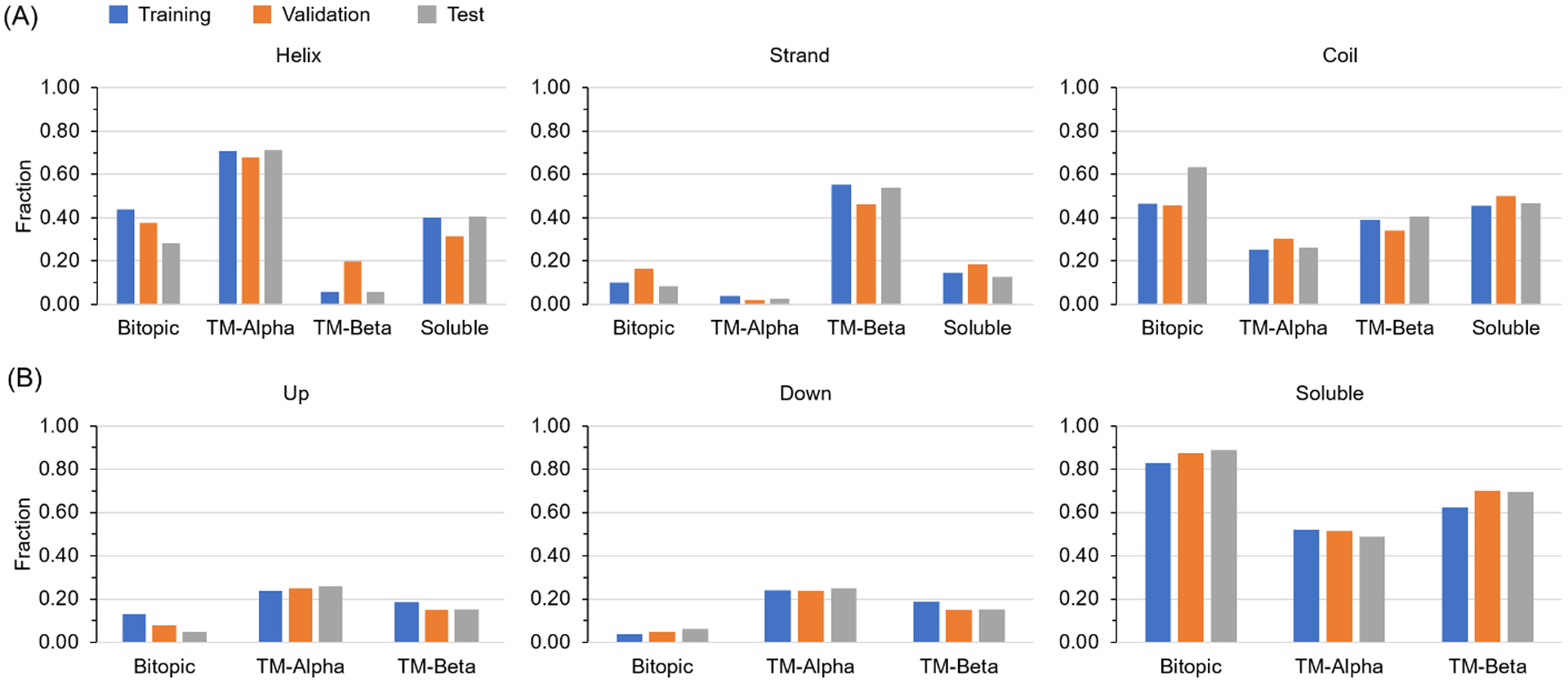
(A) The distribution of secondary structure types among training, validation, and test sets for all four protein classes. (B) The distribution of residue topology types among training, validation, and test sets for three protein classes. The distribution for soluble proteins is omitted because the topology types of all soluble protein residues are labeled as “s”.

MASSP accurately predicts residue-level attributes

We evaluated the performance of MASSP using the Q3 (or Q2 in the case of residue location prediction) and the fractional segment overlap (SOV) accuracy measures. Q3 is the percentage of correctly predicted residues on all three types of secondary structure, transmembrane topology, or in the case of TM-beta proteins, residue orientation. The SOV measure counts the fractional extent to which predicted and experimental segments of secondary structure or transmembrane region overlap, with some allowance for non-matching residues at the ends^50,51 (see Methods).

Overall, MASSP achieves accurate simultaneous prediction of residue-level secondary structure, orientation, and transmembrane topology, with Q3s of 0.844, 0.944, and 0.928, respectively, over 19416 test set residues (Fig. 3A). The Q2 accuracy for residue location prediction over the same set of residues is 0.946. When the overall accuracy was decomposed according to protein classes, MASSP achieved the highest secondary structure prediction Q3 for TM-alpha proteins (0.884) and the lowest for soluble proteins (0.809) (Fig. 3B). This is likely because the lipid bilayer imposes several constraints on structures of integral membrane proteins, simplifying their secondary structure prediction. Remarkably, MASSP rarely predicts residues of soluble proteins to be membrane associated, as manifested by the near perfect accuracy in predicting location, orientation, and topology of residues of soluble proteins (Fig. 3B). Among the three classes of membrane associated proteins, the three membrane related attributes are much easier to predict for both bitopic and TM-beta proteins than for TM-alpha proteins. This is likely because the folds of TM-alpha proteins are generally much more complex than bitopic or TM-beta proteins.

Figure 3. Performance of MASSP on predicting structural features as tested using a held-out test set.

(A) Overall accuracy achieved by MASSP for each target attribute. (B) Overall accuracy for each target attribute decomposed according to protein class. (C) Distribution of prediction accuracy for each target attribute on test set proteins. (D) Distribution of SOV metric for each target attribute on test set proteins.

We also computed the per-protein distributions of the Q3 and the SOV measures (Fig. 3C and 3D). For secondary structure prediction, the median Q3 and SOV are 0.845 and 0.792, respectively. For the other three membrane protein-related attributes, the median accuracies for location, orientation, and topology are 0.881, 0.890, and 0.867, and the median SOVs are 0.755, 0.803, and 0.852, respectively, across 36 membrane proteins in the test set. These results indicate that MASSP achieved excellent performance in predicting residue-level attributes.

Accurate prediction of protein classes via a LSTM neural network

Knowing the structural class of a protein (soluble vs. transmembrane, TM-alpha vs. TM-beta, and bitopic vs. multi-spanning) is essential toward understanding its potential cellular function. MASSP builds on the residue-level predictions of secondary structures, membrane associations, residue orientations, and transmembrane topologies and leverages the power of the LSTM recurrent neural network architecture⁵³ to accurately predict protein classes. In this LSTM model, each sequence is treated as a single data point and is processed by iterating through the sequence elements and maintaining a state containing information relative to what it has seen so far. When applied to protein class prediction, the network maintains information about all residues in the sequence. This is akin to sentiment analysis in natural language processing⁴⁸. To achieve this, we tokenize protein sequences at residue level by representing each residue with a “word” composed of their residue-level predictions. For instance, a residue predicted to be helix-forming (H), membrane associated (M), lipid facing (L), and going toward the cytoplasmic side (D) would be represented by the word “HMLD”, and a strand-forming (E) residue in a soluble protein would be represented by the word “Esss”. As shown in Table 1, the LSTM model achieved a notable four-class classification accuracy of 98.6%. Specifically, it correctly classified all bitopic, TM-alpha, and soluble proteins. The only mis-classified protein in the held-out test set is the pore-forming TM-beta subunit 7ahlA, which has a predominantly large soluble domain (95.9% of all residues are outside the membrane). Our results suggest a remarkable effectiveness of LSTM neural networks in predicting protein classes by learning from predicted residue-level attributes that are combined in a residue-wise manner.

Table 1.

Summary of the performance of the LSTM-based protein class predictor.

	Bitopic	TM-alpha	TM-beta	Soluble
Bitopic	5	0	0	0
TM-alpha	0	23	0	0
TM-beta	0	0	7	1
Soluble	0	0	0	37

Row headers indicate true protein classes; column headers indicate predicted protein classes; numbers in the matrices are protein counts.

MASSP achieves state-of-the-art performance

We evaluated the performance of MASSP relative to other methods in the field using the same test set. We first compared it to Jufo9D, which was previously developed in our group⁵⁴, and five other popular secondary structure prediction methods (PSIPRED¹¹, RaptorX-Property⁵⁵, SPINE-X^56,57, NetSurfP-2.0⁵⁸, and TMP-SS³⁴). MASSP performs comparably or better than all secondary structure prediction methods evaluated in this work (Figure 4). Specifically, MASSP achieved a median Q3 of 0.845, which is comparable to the best method NetSurfP-2.0 (0.850), but substantially better than PSIPRED (0.829), SPINE-X (0.819), RaptorX-Property (0.750), TMP-SS (0.821). Our previous method Jufo9D achieved a moderate median Q3 of 0.766. We note that due to the unavailability of NetSurfP-2.0 training set, we were not able to check if any proteins used to train NetSurfP-2.0 was in our test set (No downloadable training data at https://services.healthtech.dtu.dk/service.php?NetSurfP-2.0, last accessed April. 13^th 2021). We also compared these methods in terms of the SOV metric. With a median SOV of 0.792, MASSP is ranked the best among all evaluated methods and is substantially better than TMP-SS (0.768) and NetSurfP-2.0 (0.729) whose SOVs are ranked next. PSIPRED (0.690) and SPINE-X (0.705) performed similarly in both evaluations, while RaptorX-Property (0.651) was significantly worse. Our evaluation also indicates that Jufo9D has the lowest SOVs.

Figure 4. MASSP predicts secondary structure accurately.

(A) Distribution of Q3 secondary structure accuracies of MASSP on the test set compared to six other representative methods. (B) Distribution of performance at secondary structure prediction in terms of the SOV metric for MASSP and six other representative methods.

We then compared the performance of MASSP with six other commonly used methods (JUFO9D⁵⁴, MEMSAT3³⁰, OCTOPUS³¹, TMHMM2⁵⁹, TMP-SS³⁴, and TOPCONS2⁶⁰) in predicting transmembrane segments and topology for TM-alpha and bitopic proteins (Tables 2 and 3). Our comparison shows that MASSP has the best performance in predicting the number and location of TMHs. MASSP correctly identified 151 out of all 154 TMHs that are at least 10 residues long, ~9% higher than the MEMSAT3 and OCTOPUS, which are the second best. For topology prediction, OCTOPUS performs the best both at the protein level and residue level for both TM-alpha and bitopic proteins. OCTOPUS only mis-predicted the topology of 1 bitopic protein, whereas MASSP mis-predicted the topology of 1 TM-alpha and 2 bitopic proteins. At the residue level, MASSP attained a Q3 of 0.871 and SOV of 0.850 for TM-alpha proteins, which are comparable to OCTOPUS (Q3: 0.874, SOV: 0.861). However, MASSP’s residue-level performance is substantially lower than OCTOPUS for bitopic proteins, due to its worse prediction of protein-level topology.

Table 2.

Comparison on the performance of TMH and topology prediction for TM-alpha proteins (23 proteins in total).

Method	Correct #TMH	Correct topology	Q3	SOV
Jufo9D	131 / 149 (87.9%)	NA	NA	NA
MASSP	146 / 149 (98.0%)	22 / 23 (95.6%)	0.871	0.850
MEMSAT3	134 / 149 (89.9%)	20 / 23 (87.0%)	0.851	0.813
OCTOPUS	134 / 149 (89.9%)	23 / 23 (100%)	0.874	0.861
TMHMM2	129 / 149 (86.6%)	16 / 23 (69.7%)	0.790	0.772
TMP-SS	130 / 138 (94.2%)	NA	NA	NA
TOPCONS2	130 / 149 (87.2%)	20 / 23 (87.0%)	0.830	0.801

NA: not available, Jufo9D and TMP-SS do not predict residue-level three-state topology. A predicted TMH is considered correct if it overlaps with the true TMH for at least 10 residues. Our local run of TMP-SS was not successful for 3dh4A, hence the total number of TMHs is 138.

Table 3.

Comparison on the performance of TMH and topology prediction for bitopic transmembrane proteins (5 proteins in total).

Method	Correct #TMH	Correct topology	Q3	SOV
Jufo9D	4 / 5	NA	NA	NA
MASSP	5 / 5	3 / 5	0.551	0.531
MEMSAT3	4 / 5	4 / 5	0.831	0.819
OCTOPUS	4 / 5	4 / 5	0.865	0.869
TMHMM2	4 / 5	3 / 5	0.629	0.630
TMP-SS	5 / 5	NA	NA	NA
TOPCONS2	3 / 5	4 / 5	0.589	0.584

NA: not available, Jufo9D and TMP-SS do not predict residue-level three-state topology. A predicted TMH is considered correct if it overlaps with the true TMH for at least 10 residues.

We next compared the performance of MASSP in predicting TM strands of TM-beta proteins with Jufo9D⁵⁴, BOCTOPUS2³², and PRED-TMBB2³³. The latter two methods were recently developed methods and were shown to have improved performance over previous methods. As shown in Table 4, MASSP achieved the highest accuracy (Q3: 0.775, SOV: 0.775) in residue-level topology prediction and in predicting the number and location of TM strands (98 out of 104 TM strands that have at least 5 residues). BOCTOPUS2 correctly predicted the highest number of protein-level topology (6 out of the 8 TM-beta proteins in the held-out test set) and achieved the same level of accuracy as MASSP in predicting the number and location of TM strands. However, the residue-level accuracy of BOCTOPUS2 (Q3: 0.696, SOV: 0.745) is substantially worse than MASSP.

Table 4.

Comparison on the performance of TMS and topology prediction for TM-beta proteins (8 proteins int total).

Method	Correct #TMS	Correct topology	Q3	SOV
Jufo9D	82 / 104 (78.8%)	NA	NA	NA
MASSP	98 / 104 (94.1%)	5 (64.3%)	0.775	0.775
BOCTOPUS2	98 / 104 (94.1%)	6 (75.0%)	0.696	0.745
PRED-TMBB2	85 / 104 (81.7%)	5 (64.3%)	0.714	0.716

NA: not available, Jufo9D does not predict residue-level three-state topology. A predicted TMS is considered correct if it overlaps with the true TMS for at least 5 residues.

In summary, our extensive comparison on secondary structure and membrane association/topology prediction tasks demonstrates that MASSP performance is comparable to or better than state-of-the-art methods, while being more versatile and applicable to any protein sequences.

Examples of accurate MASSP predictions

We demonstrate the predictions made by MASSP on two proteins by mapping secondary structures and topologies predicted by MASSP onto tertiary structures (Fig. 5). We selected the subunit B from the caa3-type cytochrome oxidases from Thermus thermophilus (PDB ID: 2yevB) and the TamA protein from the E. coli (PDB ID: 4c00A) as two representative examples, because they both consist of large transmembrane and soluble domains and all three types of secondary structures are also well represented. The subunit B from the caa3-type cytochrome oxidases consists of an alpha-helical TM domain and a large extracellular soluble domain, resolved at a resolution of 2.4 Å. TamA is an E. coli Omp85 protein involved in autotransporter biogenesis. It comprises a 16-stranded transmembrane β-barrel and three cytoplasmic POTRA domains, resolved at a resolution of 2.3 Å. For 2yevB, MASSP achieved a Q3 of 0.936 and a SOV of 0.893 for secondary structure prediction, and Q3 of 0.984 and a SOV of 0.977 for topology prediction. For 4c00A, MASSP achieved a Q3 of 0.815 and a SOV of 0.780 for secondary structure prediction, and Q3 of 0.938 and a SOV of 0.911 for topology prediction. These two examples illustrate that even for proteins composed of mixed large transmembrane and soluble domains, MASSP can accurately predict both secondary structures and transmembrane topologies.

Figure 5. Examples of accurate secondary structure and transmembrane topology prediction by MASSP.

(A) Comparisons of experimental and predicted secondary structures mapped to tertiary structures for cytochrome C oxidase subunit 2 (PDB: 2yevB) and translocation and assembly module subunit TamA (PDB: 4c00A) illustrating high accuracy. (B) Comparisons of experimental and predicted residue topologies mapped to tertiary structure for the same proteins.

Discussion

Prediction of secondary structures and transmembrane regions are fundamental problems in bioinformatics with broad downstream applications. Decades of research into these problems have produced dozens of methods that can be broadly categorized into knowledge-based analyses, generative probabilistic modeling, and discriminative machine learning. However, methods with better performance are still needed giving the increasingly large gap between the set of known sequences and known structures^5,22. Among machine-learning methods, those mainly based on neural networks, have been shown to generally perform best, with Q3 accuracies for secondary structure prediction around 80%⁵; however, their accuracies in predicting transmembrane segments and topologies have been low²². A newly sequenced protein can be of any one of the structural classes of soluble, bitopic, TM-alpha, or TM-beta. Thus, methods are needed for simultaneous prediction of secondary structures, transmembrane regions, topologies, and protein class.

In this work, we introduced MASSP, a multi-task deep-learning framework designed for simultaneous prediction of secondary structures, transmembrane regions, topologies, and protein classes. MASSP simultaneously predicts residue-level structural attributes for all four classes of proteins. The core algorithm behind MASSP is a two-tier deep neural network. Our framework is conceptually similar to several recent works that reported substantially improved performances in predicting signal peptides⁶¹, protein subcellular localization⁶², the topology of TM-alpha proteins³⁵. The first tier is a multi-layer multi-task 2D-CNN that predicts residue-level 1D structural attributes. The second tier is a LSTM neural network that treats the predictions of the first tier from the perspective of natural language and predicts the protein class of the input amino acid sequence. We demonstrated that MASSP accurately predicts residue-level secondary structures, locations, orientations, and residue topologies, and protein-level structural classes. We also show that the performance of MASSP is comparable or better than several widely used methods for secondary structure and membrane topology prediction.

In addition to performance that is better than or comparable to existing methods, the MASSP framework has several other important strengths. First, the multi-tasking nature of MASSP makes it a versatile tool that simultaneously predicts residue-level 1D structural features. Specifically, the multi-output architecture of the 2D-CNN would allow us to easily extend MASSP to predict other structural properties, such as solvent accessibility and contact order, from amino acid sequence without the requirement of training a different network for each target property. Second, the fact that MASSP does not make a priori assumptions about whether the given amino acid sequence represents a TM-alpha protein, TM-beta protein, or a soluble protein gives the user a one-stop shop where the secondary structures and membrane associations of a given amino acid sequence of any protein class can be predicted. Thus, MASSP could be applied to wholly sequenced proteomes of an organism to predict the protein class composition of the proteome as well as residue-level secondary structures and membrane associations.

Despite half-a-century of research into the problems of secondary structure prediction and transmembrane segment and topology prediction, these problems are still open and the field seems to have reached a bottleneck where improvement in prediction accuracy is small and progress is slow⁵. It strikes us as remarkable that the approach that we took in developing MASSP, i.e. learning patterns in PSSMs with deep 2D-CNNs, achieved comparable or better performance than previously developed, more sophisticated methods. This can be partially attributed to applying the “right” type of neural network to the “right” representation of input features, i.e. we leveraged the image-processing power inherent in 2D-CNNs and the fact that PSSMs can be thought of images with real-valued “pixels”. Recent advances in protein tertiary structure prediction also demonstrated that a boost in performance can be achieved by developing novel neural network architectures that leverage the problem’s fundamental mathematical essence^4,63–65. For example, AlphaFold, the algorithm that outperformed all entrants in CASP13, relies on the fundamental principle of the interconvertibility of probability and energy, and predicts the probability distributions of residue pair distances and converts distance distributions to energy landscapes^4,64. In the recent CASP14 competition, AlphaFold2, which is based on an attention-based neural network system, trained end-to-end, that attempts to interpret protein structures as “spatial graphs”, outperformed all its competitors with an unprecedented margin^2,66. These advances in tertiary structure prediction together with our work here suggest that completely solving these problems will likely require the development novel neural network architectures and representation of input features.

References

- (1).Li B; Fooksa M; Heinze S; Meiler J Finding the needle in the haystack: towards solving the protein-folding problem computationally. Crit Rev Biochem Mol Biol 2018, 53 (1), 1–28. [DOI] [PMC free article] [PubMed] [Google Scholar]
- (2).Jumper J; Evans R; Pritzel A; Green T; Figurnov M; Tunyasuvunakool K; Ronneberger O; Bates R; Žídek A; Bridgland A et al. Fourteenth Critical Assessment of Techniques for Protein Structure Prediction, 2020.
- (3).Shrestha R; Fajardo E; Gil N; Fidelis K; Kryshtafovych A; Monastyrskyy B; Fiser A Assessing the accuracy of contact predictions in CASP13. Proteins 2019, 87 (12), 1058–1068. [DOI] [PMC free article] [PubMed] [Google Scholar]
- (4).Senior AW; Evans R; Jumper J; Kirkpatrick J; Sifre L; Green T; Qin C; Zidek A; Nelson AWR; Bridgland A et al. Improved protein structure prediction using potentials from deep learning. Nature 2020, 577 (7792), 706–710. [DOI] [PubMed] [Google Scholar]
- (5).Yang Y; Gao J; Wang J; Heffernan R; Hanson J; Paliwal K; Zhou Y Sixty-five years of the long march in protein secondary structure prediction: the final stretch? Brief Bioinform 2018, 19 (3), 482–494. [DOI] [PMC free article] [PubMed] [Google Scholar]
- (6).Torrisi M; Pollastri G; Le Q Deep learning methods in protein structure prediction. Comput Struct Biotechnol J 2020, 18, 1301–1310. [DOI] [PMC free article] [PubMed] [Google Scholar]
- (7).Chou PY; Fasman GD Prediction of protein conformation. Biochemistry 1974, 13 (2), 222–245. [DOI] [PubMed] [Google Scholar]
- (8).Frishman D; Argos P Seventy-five percent accuracy in protein secondary structure prediction. Proteins 1997, 27 (3), 329–335. [DOI] [PubMed] [Google Scholar]
- (9).Garnier J; Gibrat JF; Robson B GOR method for predicting protein secondary structure from amino acid sequence. Methods Enzymol 1996, 266, 540–553. [DOI] [PubMed] [Google Scholar]
- (10).Rost B; Sander C Prediction of protein secondary structure at better than 70% accuracy. J Mol Biol 1993, 232 (2), 584–599. [DOI] [PubMed] [Google Scholar]
- (11).Jones DT Protein secondary structure prediction based on position-specific scoring matrices. J Mol Biol 1999, 292 (2), 195–202. [DOI] [PubMed] [Google Scholar]
- (12).Rost B PHD: predicting one-dimensional protein structure by profile-based neural networks. Methods Enzymol 1996, 266, 525–539. [DOI] [PubMed] [Google Scholar]
- (13).Qian N; Sejnowski TJ Predicting the secondary structure of globular proteins using neural network models. J Mol Biol 1988, 202 (4), 865–884. [DOI] [PubMed] [Google Scholar]
- (14).Rost B; Sander C Prediction of Protein Secondary Structure at Better Than 70-Percent Accuracy. Journal of Molecular Biology 1993, 232 (2), 584–599. [DOI] [PubMed] [Google Scholar]
- (15).Rost B; Sander C Improved prediction of protein secondary structure by use of sequence profiles and neural networks. Proc Natl Acad Sci U S A 1993, 90 (16), 7558–7562. [DOI] [PMC free article] [PubMed] [Google Scholar]
- (16).Meiler J; Zeidler A; Schmaschke F; Muller M Generation and evaluation of dimension-reduced amino acid parameter representations by artificial neural networks. Journal of Molecular Modeling 2001, 7 (9), 360–369. [Google Scholar]
- (17).Meiler J; Baker D Coupled prediction of protein secondary and tertiary structure. Proc Natl Acad Sci U S A 2003, 100 (21), 12105–12110. [DOI] [PMC free article] [PubMed] [Google Scholar]
- (18).LeCun Y; Bengio Y; Hinton G Deep learning. Nature 2015, 521 (7553), 436–444. [DOI] [PubMed] [Google Scholar]
- (19).Wang S; Peng J; Ma J; Xu J Protein Secondary Structure Prediction Using Deep Convolutional Neural Fields. Sci Rep 2016, 6, 18962. [DOI] [PMC free article] [PubMed] [Google Scholar]
- (20).Zhavoronkov A; Ivanenkov YA; Aliper A; Veselov MS; Aladinskiy VA; Aladinskaya AV; Terentiev VA; Polykovskiy DA; Kuznetsov MD; Asadulaev A et al. Deep learning enables rapid identification of potent DDR1 kinase inhibitors. Nat Biotechnol 2019, 37 (9), 1038–1040. [DOI] [PubMed] [Google Scholar]
- (21).Liu S; Xu LY; Guan FH; Liu YT; Cui YX; Zhang Q; Zheng X; Bi GQ; Zhou ZH; Zhang XK et al. Cryo-EM structure of the human alpha 5 beta 3 GABA(A) receptor. Cell Res 2018, 28 (9), 958–961. [DOI] [PMC free article] [PubMed] [Google Scholar]
- (22).Koehler Leman J; Ulmschneider MB; Gray JJ Computational modeling of membrane proteins. Proteins 2015, 83 (1), 1–24. [DOI] [PMC free article] [PubMed] [Google Scholar]
- (23).Fleishman SJ; Ben-Tal N Progress in structure prediction of alpha-helical membrane proteins. Curr Opin Struct Biol 2006, 16 (4), 496–504. [DOI] [PubMed] [Google Scholar]
- (24).Kyte J; Doolittle RF A simple method for displaying the hydropathic character of a protein. J Mol Biol 1982, 157 (1), 105–132. [DOI] [PubMed] [Google Scholar]
- (25).von Heijne G The Distribution of Positively Charged Residues in Bacterial Inner Membrane-Proteins Correlates with the Trans-Membrane Topology. Embo Journal 1986, 5 (11), 3021–3027. [DOI] [PMC free article] [PubMed] [Google Scholar]
- (26).von Heijne G Membrane-Protein Structure Prediction - Hydrophobicity Analysis and the Positive-inside Rule. Journal of Molecular Biology 1992, 225 (2), 487–494. [DOI] [PubMed] [Google Scholar]
- (27).Rost B; Casadio R; Fariselli P; Sander C Transmembrane helices predicted at 95% accuracy. Protein Sci 1995, 4 (3), 521–533. [DOI] [PMC free article] [PubMed] [Google Scholar]
- (28).Rost B; Fariselli P; Casadio R Topology prediction for helical transmembrane proteins at 86% accuracy. Protein Sci 1996, 5 (8), 1704–1718. [DOI] [PMC free article] [PubMed] [Google Scholar]
- (29).Tusnady GE; Simon I Principles governing amino acid composition of integral membrane proteins: application to topology prediction. J Mol Biol 1998, 283 (2), 489–506. [DOI] [PubMed] [Google Scholar]
- (30).Jones DT Improving the accuracy of transmembrane protein topology prediction using evolutionary information. Bioinformatics 2007, 23 (5), 538–544. [DOI] [PubMed] [Google Scholar]
- (31).Viklund H; Elofsson A OCTOPUS: improving topology prediction by two-track ANN-based preference scores and an extended topological grammar. Bioinformatics 2008, 24 (15), 1662–1668. [DOI] [PubMed] [Google Scholar]
- (32).Hayat S; Peters C; Shu N; Tsirigos KD; Elofsson A Inclusion of dyad-repeat pattern improves topology prediction of transmembrane beta-barrel proteins. Bioinformatics 2016, 32 (10), 1571–1573. [DOI] [PubMed] [Google Scholar]
- (33).Tsirigos KD; Elofsson A; Bagos PG PRED-TMBB2: improved topology prediction and detection of beta-barrel outer membrane proteins. Bioinformatics 2016, 32 (17), i665–i671. [DOI] [PubMed] [Google Scholar]
- (34).Liu Z; Gong Y; Bao Y; Guo Y; Wang H; Lin GN TMPSS: A Deep Learning-Based Predictor for Secondary Structure and Topology Structure Prediction of Alpha-Helical Transmembrane Proteins. Front Bioeng Biotechnol 2020, 8, 629937. [DOI] [PMC free article] [PubMed] [Google Scholar]
- (35).Yang Y; Yu J; Liu Z; Wang X; Wang H; Ma Z; Xu D An Improved Topology Prediction of Alpha-Helical Transmembrane Protein Based on Deep Multi-Scale Convolutional Neural Network. IEEE/ACM Trans Comput Biol Bioinform 2020, PP. [DOI] [PubMed] [Google Scholar]
- (36).Li B; Mendenhall J; Nguyen ED; Weiner BE; Fischer AW; Meiler J Improving prediction of helix-helix packing in membrane proteins using predicted contact numbers as restraints. Proteins 2017, 85 (7), 1212–1221. [DOI] [PMC free article] [PubMed] [Google Scholar]
- (37).Fischer AW; Heinze S; Putnam DK; Li B; Pino JC; Xia Y; Lopez CF; Meiler J CASP11--An Evaluation of a Modular BCL::Fold-Based Protein Structure Prediction Pipeline. PLoS One 2016, 11 (4), e0152517. [DOI] [PMC free article] [PubMed] [Google Scholar]
- (38).Lomize MA; Lomize AL; Pogozheva ID; Mosberg HI OPM: orientations of proteins in membranes database. Bioinformatics 2006, 22 (5), 623–625. [DOI] [PubMed] [Google Scholar]
- (39).Wang G; Dunbrack RL Jr. PISCES: a protein sequence culling server. Bioinformatics 2003, 19 (12), 1589–1591. [DOI] [PubMed] [Google Scholar]
- (40).Kabsch W; Sander C Dictionary of protein secondary structure: pattern recognition of hydrogen-bonded and geometrical features. Biopolymers 1983, 22 (12), 2577–2637. [DOI] [PubMed] [Google Scholar]
- (41).Heinig M; Frishman D STRIDE: a web server for secondary structure assignment from known atomic coordinates of proteins. Nucleic Acids Res 2004, 32 (Web Server issue), W500–502. [DOI] [PMC free article] [PubMed] [Google Scholar]
- (42).Majumdar I; Krishna SS; Grishin NV PALSSE: a program to delineate linear secondary structural elements from protein structures. BMC Bioinformatics 2005, 6, 202. [DOI] [PMC free article] [PubMed] [Google Scholar]
- (43).Lomize MA; Pogozheva ID; Joo H; Mosberg HI; Lomize AL OPM database and PPM web server: resources for positioning of proteins in membranes. Nucleic Acids Research 2012, 40 (D1), D370–D376. [DOI] [PMC free article] [PubMed] [Google Scholar]
- (44).Woodall NB; Hadley S; Yin Y; Bowie JU Complete topology inversion can be part of normal membrane protein biogenesis. Protein Sci 2017, 26 (4), 824–833. [DOI] [PMC free article] [PubMed] [Google Scholar]
- (45).Fluman N; Tobiasson V; von Heijne G Stable membrane orientations of small dual-topology membrane proteins. Proc Natl Acad Sci U S A 2017, 114 (30), 7987–7992. [DOI] [PMC free article] [PubMed] [Google Scholar]
- (46).Altschul SF; Madden TL; Schaffer AA; Zhang J; Zhang Z; Miller W; Lipman DJ Gapped BLAST and PSI-BLAST: a new generation of protein database search programs. Nucleic Acids Res 1997, 25 (17), 3389–3402. [DOI] [PMC free article] [PubMed] [Google Scholar]
- (47).Remmert M; Biegert A; Hauser A; Söding J HHblits: lightning-fast iterative protein sequence searching by HMM-HMM alignment. Nat Methods 2012, 9 (2), 173–175. [DOI] [PubMed] [Google Scholar]
- (48).Chollet F Deep Learning with Python; Manning Pulications: Shelter Island, NY, 2018. [Google Scholar]
- (49).Kingma DP; Ba J, 2014.
- (50).Rost B; Sander C; Schneider R Redefining the Goals of Protein Secondary Structure Prediction. Journal of Molecular Biology 1994, 235 (1), 13–26. [DOI] [PubMed] [Google Scholar]
- (51).Zemla A; Venclovas C; Fidelis K; Rost B A modified definition of Sov, a segment-based measure for protein secondary structure prediction assessment. Proteins 1999, 34 (2), 220–223. [DOI] [PubMed] [Google Scholar]
- (52).Liu T; Wang Z SOV_refine: A further refined definition of segment overlap score and its significance for protein structure similarity. Source Code Biol Med 2018, 13, 1. [DOI] [PMC free article] [PubMed] [Google Scholar]
- (53).Hochreiter S; Schmidhuber J Long short-term memory. Neural Comput 1997, 9 (8), 1735–1780. [DOI] [PubMed] [Google Scholar]
- (54).Leman JK; Mueller R; Karakas M; Woetzel N; Meiler J Simultaneous prediction of protein secondary structure and transmembrane spans. Proteins 2013, 81 (7), 1127–1140. [DOI] [PMC free article] [PubMed] [Google Scholar]
- (55).Buchan DWA; Jones DT The PSIPRED Protein Analysis Workbench: 20 years on. Nucleic Acids Res 2019, 47 (W1), W402–W407. [DOI] [PMC free article] [PubMed] [Google Scholar]
- (56).Wang S; Li W; Liu S; Xu J RaptorX-Property: a web server for protein structure property prediction. Nucleic Acids Res 2016, 44 (W1), W430–435. [DOI] [PMC free article] [PubMed] [Google Scholar]
- (57).Faraggi E; Zhang T; Yang Y; Kurgan L; Zhou Y SPINE X: improving protein secondary structure prediction by multistep learning coupled with prediction of solvent accessible surface area and backbone torsion angles. J Comput Chem 2012, 33 (3), 259–267. [DOI] [PMC free article] [PubMed] [Google Scholar]
- (58).Klausen MS; Jespersen MC; Nielsen H; Jensen KK; Jurtz VI; Sonderby CK; Sommer MOA; Winther O; Nielsen M; Petersen B et al. NetSurfP-2.0: Improved prediction of protein structural features by integrated deep learning. Proteins 2019, 87 (6), 520–527. [DOI] [PubMed] [Google Scholar]
- (59).Kall L; Krogh A; Sonnhammer ELL A combined transmembrane topology and signal peptide prediction method. Journal of Molecular Biology 2004, 338 (5), 1027–1036. [DOI] [PubMed] [Google Scholar]
- (60).Tsirigos KD; Peters C; Shu N; Kall L; Elofsson A The TOPCONS web server for consensus prediction of membrane protein topology and signal peptides. Nucleic Acids Res 2015, 43 (W1), W401–407. [DOI] [PMC free article] [PubMed] [Google Scholar]
- (61).Almagro Armenteros JJ; Tsirigos KD; Sonderby CK; Petersen TN; Winther O; Brunak S; von Heijne G; Nielsen H SignalP 5.0 improves signal peptide predictions using deep neural networks. Nat Biotechnol 2019, 37 (4), 420–423. [DOI] [PubMed] [Google Scholar]
- (62).Almagro Armenteros JJ; Sonderby CK; Sonderby SK; Nielsen H; Winther O DeepLoc: prediction of protein subcellular localization using deep learning. Bioinformatics 2017, 33 (21), 3387–3395. [DOI] [PubMed] [Google Scholar]
- (63).Xu J Distance-based protein folding powered by deep learning. Proc Natl Acad Sci U S A 2019, 116 (34), 16856–16865. [DOI] [PMC free article] [PubMed] [Google Scholar]
- (64).AlQuraishi M A watershed moment for protein structure prediction. Nature 2020, 577 (7792), 627–628. [DOI] [PubMed] [Google Scholar]
- (65).AlQuraishi M End-to-End Differentiable Learning of Protein Structure. Cell Syst 2019, 8 (4), 292–301 e293. [DOI] [PMC free article] [PubMed] [Google Scholar]
- (66).Dauparas J; Fuchs F; https://fabianfuchsml.github.io/alphafold2/, 2021; Vol. 2021.
Associated Data
This section collects any data citations, data availability statements, or supplementary materials included in this article.