Contact tracing as a measure to combat COVID-19 and other infectious diseases

Abstract

Background

Most of the mathematical modeling studies on COVID-19 transmission are based on continuous deterministic models that do not consider the characteristics of social networks.

Methods

The effect of contact tracing on mitigating COVID-19, and other infectious diseases in general, is studied in a small-world network. This network has its advantages over the commonly used continuous deterministic mathematical models in that the characteristics of social networks can be properly incorporated.

Results

Simulation results show that for the original strain of SARS-CoV-2, contact tracing can play an important role in reducing and delaying the peak daily new cases. New cases can be reduced by using symptom onset to isolate tracked individuals, but the benefit can be greatly enhanced by testing asymptomatic and presymptomatic individuals on the sixth to eighth day of infection. For the delta variant, or other variants of much higher infectivity, contact tracing alone cannot significantly lower the number of daily new cases but is able to delay the peaks greatly, thus affording more time to explore and implement pharmaceutical interventions.

Conclusions

Contact tracing can be a very powerful tool to combat COVID-19 caused by the original strain or any variant of SARS-CoV-2. In order to make contact tracing effective, every effort is needed to expand the pool of contact tracing and provide all necessary support to the self-quarantined.

Nonpharmaceutical Interventions (NPIs), such as facemask wearing, business and school lockdowns, and contact tracing, are effective tools to combat infectious diseases such as COVID-19 that have devastated people's lives around the globe.¹ When a vaccine is not available, NPIs can help “flatten the curve” which helps gain valuable time to develop, manufacture, and distribute the vaccine. Even after a significant fraction, or even most, of the general population has been vaccinated, breakthrough infection by new variants of the virus among vaccinated people may still pose imminent threats,² and NPIs can play an important role to combat the spread of infections. A vivid example is the delta variant of the new coronavirus (SARS-CoV-2) that caused significant breakthrough infections among the fully vaccinated population in the summer of 2021. Although contact tracing imposes restrictions and greatly disrupts the normal lives of those who are quarantined, compared to other NPIs, it is still probably the least intrusive and the most economical since it does not interfere with most of the population.

Mathematical modeling plays an essential role in combating infectious diseases.³ Modeling results provide insight to how various NPIs slow down the spread of infections and rationalize when to initialize and terminate the NPIs. Up to now, most of the epidemiological modeling works are based on continuous deterministic compartment models.^{3 , 4} An example is the popular continuous SIR model in which the general population is distributed in 3 compartments: susceptible, infectious, and recovered. Of course, different variants of SIR models allow different or additional states such as reinfected, latent, etc. An intrinsic and vital shortcoming of the continuous deterministic models is that the infection transmission is assumed to be homogeneous,⁵ that is, all susceptible people have equal chances of getting infected by a given infectious person regardless of whether they have direct contact with the infected. More fundamentally, continuous deterministic models fail to take into consideration the interactions among people in society since no contact network can be homogeneous. This deficiency inevitably diminishes the validity of the modeling results.

The homogeneous assumption associated with the continuous deterministic compartment models can be avoided if the spread of infectious diseases is studied in complex networks.⁶ For infectious disease transmissions, several important metrics of the networks must be taken into consideration. The first is the shortest path length that characterizes the distance among vertices in the network. Another is the clustering coefficient that represents the relative propensity of 2 vertices, given that they share a common neighbor (in the layman's words, a friend's friend is likely a friend). The third is the degree distribution which reflects that some vertices have more connected vertices than others. There are 2 types of networks that possess 2 (out of 3) ideal characteristics. Scale-free networks have the right short distances among vertices and a scale-free degree distribution which is supposed to be the correct feature for social networks, but their clustering coefficients are usually too small.⁷ On the other hand, small-world networks have the correct short distances among vertices and a high clustering coefficient, but they have an exponential degree distribution.⁸ It is true that certain scale-free networks can be designed to have the right clustering coefficient, but at the same time, doing so will introduce unwanted features into the networks. For example, a scale-free network can be developed to have the correct short distances among vertices and a high clustering coefficient, but some vertices in the network are connected to all other vertices,⁹ a feature that does not resemble social networks. Additionally, a recent study has shown that social networks are not necessarily scale-free, and many of them are at best weakly scale-free.¹⁰ This implies that a scale-free network may not be the best choice as the paradigm on which infection transmission is studied.

It is the author's choice to use a small-world network to study the infection transmission and in particular, the effects of contact tracing as one of the NPIs to mitigate infectious diseases such as COVID-19. As mentioned previously, 2 desirable features possessed by small-world networks are the short distances among vertices and a large clustering coefficient. It is not clear how the unappealing characteristic of non-scale-free degree distribution affects the modeling results. As such, the primary hypothesis of this study is that small-world networks can be used to study how infection spreads.

It is helpful to give a brief description of the objectives of the present study. First of all, it exposes a potentially important flaw embedded in the most widely used continuous deterministic mathematical models of infection transmission and offers a more rigorous and physically sound alternative, the small-world network model. Secondly, it demonstrates that the small-world network model can meaningfully redress the shortfall of underestimating the effectiveness of contact tracing. Thirdly, it provides insights for public health officials and the means to enhance the efficacy of contact tracing. By expanding the pool for contact tracing, testing effectively, and making every effort to ensure that all quarantined people are provided with reasonable accommodations so that they can remain in quarantine until they are cleared to go back to their normal lives.

Methods

The small-world network

The original Watts-Strogatz small-world network⁸ connects a total of N vertices along a circle by both short-range regular edges and long-range random edges. Each vertex is connected to its k neighbors on each side by regular edges, and some of these edges are re-wired randomly to connect remote vertices. The number of random edges is specified by a parameter p, which is the percentage of edges that are rewired. For example, p = .01 means that 1% of the regular edges are rewired, and those edges are called random edges. In this study, N, k, and p are set to be 100,000, 100 and 0.01. A constraint that needs to be satisfied is that $N\gg k\gg \text{ln}\left(N\right)\gg 1$ so that the network is connected by random edges.

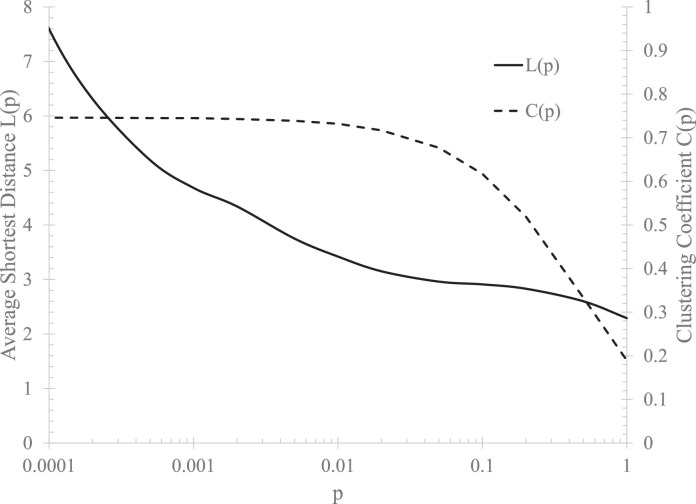
A variant¹¹ of the Watts-Strogatz model⁸ is used in the present study. Instead of rewiring regular edges to get random edges, random edges are randomly added to connect vertices to remote ones. In this variant, p signifies the ratio of random edges to total edges. Figure 1 shows that, over a wide range of p, the network model has the correct average short distance and a large clustering coefficient.

Fig 1.

The average shortest distance between vertices and clustering coefficient with N = 100,000 and k = 100.

Infection transmission in the network and epidemiological parameters

In the network, each vertex represents a person in society. The state of each vertex can be susceptible, infected, recovered, or dead. A susceptible vertex can get infected by any one of its connected infectious vertices. The newly infected goes through the recovery process in a given period of time, and during this process, it can be reclassified as dead with a probability specified as the fatality rate of the disease. In the meantime, the vertex can infect other susceptible vertices. The recovered vertex gains immunity and normally will not get infected again; however, for COVID-19, evidence exists thatimmunity can be lost.¹²

In each realization of the simulation, a randomly selected vertex is set to be infected as the index case for the outbreak. If all the infected vertices die or recover before they have a chance to infect others while most of the vertices are still susceptible, the infection is “crushed” (ie, the infection is eliminated completely from society) and the process of infection transmission stops. Otherwise, the infection continues to spread.

Several epidemiological parameters are needed in the simulation. The first one is the basic reproduction number, R ₀, which represents how contagious the disease is and quantifies, on average, the number of persons an infected person can infect when the population is almost entirely susceptible. For the original strain of SARS-CoV-2, the reported values are in the range of 2.24-3.58.^{13 , 14} To be consistent with the majority of the continuous deterministic modeling studies, it is set to be 2.5.^{3 , 15} R ₀ can be different for other variants of SARS-CoV-2. For example, the delta variant possesses a hugely different R ₀ that is estimated to be about 6.^{16 , 17}

Another parameter is the fraction of asymptomatically infected among all infected people, R _asymp. It is reported that among all the infected, 27%-57% could be asymptomatic,^{18 , 19} so in this work, I set R _asymp = 0.3. The fatality rate, R _fatality, is also highly uncertain, as in certain regions it was high but substantially lower in other regions. Without loss of generality, I assume it to be 0.05 since it accounts for only a very small fraction of the infected, so it barely changes the dynamics of the spread of disease on the network. Finally, based on epidemiological data,¹² it is assumed that a recovered individual has a probability of 20% to get reinfected within 180 days.

Infectivity profile, latent period, and incubation period

Wells et al²⁰ specified the infectivity profile for the original SARS-CoV-2 based on the database reported by He et al²¹ The profile incorporated a latent period of approximately 3 days. The same dataset reveals an average incubation period of 8.29 days. The infectivity gradually increases and peaks on day 8 after infection and then decreases until the infection is over. The entire period of infection is approximately 21 days. The latent period accommodated in the infectivity profile essentially makes the network model in alignment with an SEIR model.

Since the infectivity profile as mentioned above reflects the original SARS-CoV-2 and is consistent with R ₀ = 2.5, for a variant virus of different R ₀, the infection profile is scaled to be F _v(t) = R ₀ F _o(t)/2.5, where F _o(t) is the infection profile for the original virus.

A comprehensive review by McAloon et al²² reveals that the incubation period is log-normally distributed with m = 1.63 and s = 0.50, corresponding to an average incubation period of 5.8 days. This set of parameters is used in the present study because the 8.29- day incubation period has drawn some criticism for being unrealistically large.²³

Contact tracing

Once a decision is made to start contact tracing, all subsequently infected vertices are tagged and traced. This corresponds to the real-world situation that once some individuals are confirmed to be infected, all persons that have had meaningful close contacts with these infected individuals are contacted and instructed to take appropriate steps to reduce the chances of passing on the infection to others. Here, “meaningful” means the contact is long enough and close enough so that the virus can be transmitted from 1 person to another. The U.S. Centers for Disease Control and Prevention (CDC) issued guidance that requires the contact to be within 6 feet for at least 30 minutes. It might be argued that the guidance is too restrictive and may fail to tag and track many potentially infected people.

The individuals being tagged and tracked are to be instructed to watch for symptoms and/or take a test on a predetermined date. If symptoms show up or if the test result is positive, the individual will be put in self-quarantine for a certain period. Many jurisdictions including the CDC set the period to be 14 days.

There are 2 possible scenarios of quarantine. The first one does not involve testing and is solely based on the onset of symptoms, that is, the tagged and tracked individuals put themselves in quarantine once they exhibit certain symptoms. The second scenario involves testing which allows both the symptomatically and asymptomatically infected to be quarantined. According to Wells et al,²⁰ the optimal testing time is day 6 after being exposed to the virus.

The infection profile implies that, on average, all infected individuals recover in a period of 21 days,^{20 , 21} but in reality, this is hardly the case. Therefore, testing results should be used to determine if an individual is fully recovered and allowed to exit quarantine.

Simulation scenarios

The small-world network model is set up with N = 100,000, k = 100, and p = .01. Throughout the study, the following epidemiological parameters are chosen as follows: upon infection, the infected vertex is classified as asymptomatic with a probability of 0.3; the fatality rate among the symptomatically infected is 0.05, and the fraction of recovered vertices losing immunity in 180 days is 0.2. The functional form of the infection profile is the same as reported by Wells et al,²⁰ but in this study, it is scaled to allow different basic reproduction numbers. Additionally, the incubation period for each newly symptomatically infected vertex is randomly generated as lognormally distributed with m = 1.63 and s = 0.50.

A number of scenarios are modeled to examine the effects of various contact tracing strategies: when to start contact tracing in terms of the number of daily new cases of symptomatically infected individuals, N _start; what percentage of newly infected (including both symptomatically and asymptomatically infected) can be tracked, f _tracked; when the tracked individuals are to be isolated, t _isolated; how many individuals already have immunity when the simulation starts, N _immune – this corresponds to the situation when a new variant of virus causes an outbreak and a significant part of the population has already gained immunity either from vaccination or infection with previous strains.

In each simulation, 100 realizations are carried out so that stable statistics can be obtained for each simulation scenario.

Modeling results

Numerical simulations are conducted with 2 different basic reproduction numbers as well as different contact tracing strategies. Modeling results are organized by basic reproduction number. The first subsection presents results obtained with R ₀ (=2.5) for the original strain of SARS-CoV-2, and the second subsection shows results for the delta variant of SARS-CoV-2 which has a basic reproduction number R ₀ = 6.

R₀ = 2.5

Several factors that affect the outcome of contact tracing are studied: the time when the tracked individuals are to be isolated so that further virus transmission from them is terminated, the time to start the implementation of contact tracing in terms of the daily count of newly symptomatic cases, and the percentage of the new infection cases that can be tracked and isolated. For R ₀ = 2.5, N _immune, the number of vertices that have immunity, is assumed to be 0 since the intention of the modeling is to study the effect of contact tracing on the outbreak with the original strain of SARS-CoV-2.

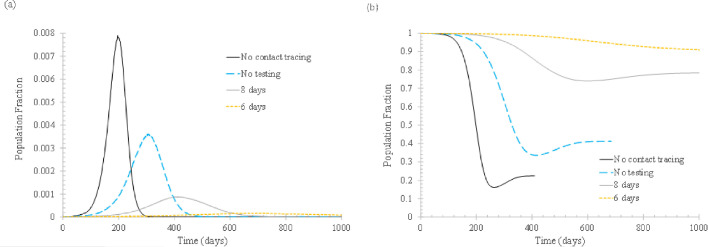
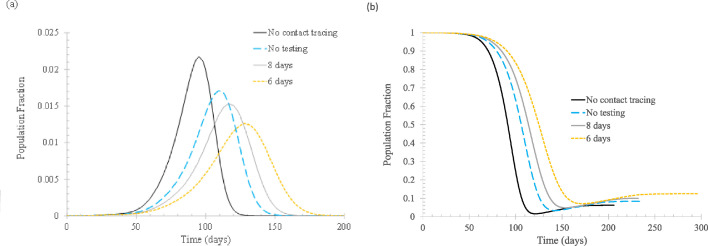
First of all, the effect of t _isolated, the time when the newly infected and tagged individuals are isolated to prevent the spread of the virus, is examined, as shown in Figure 2 . For comparison, the base case, that is, the case without implementing vertex tagging and isolation, is also shown.

Fig 2.

The effect of isolation time t_isolated. In the simulation, f_tracked = 0.5, N_start = 0, N_immune = 0. (A) Daily new cases of symptomatic infections. (B) Fraction of susceptible population. Meaning of the curve labels: no contact tracing – no vertex is tagged when infected and isolated afterwards; no testing – tagged vertices are isolated when symptoms start to appear; 8 days – tagged vertices are isolated when confirmed to be infected and the test result becomes available 8 days after infection; 6 days – similar to 8 days, but the test result is available 6 days after infection.

Clearly, contact tracing plays an important role in slowing down the spread of infection. When half of the symptomatic infections can be isolated upon symptom onset, the peak daily cases can be cut by more than a half. The effect can be further augmented if testing is conducted on the tracked individuals. If test results become available so that the infected can be isolated on the eighth day of infection, the daily new cases can be reduced significantly since both presymptomatic and asymptomatic cases can be partly isolated. If the infected can be isolated on the sixth day of infection, the effect is almost equivalent to “crush the virus,” that is, the infection transmission can be stopped. One important implication of this finding is, for the original strain of SARS-CoV-2 (its basic reproduction number has been widely shown to be around 2.5), the 50% tracking rate is not reachable since “crush the virus” is rarely seen as the outcome of implementing all NPIs. Thus, it is impossible that contact tracing alone can be as effective as implementing all NPI measures.

Figure 2(B) shows that with more infected individuals being isolated, more people remain susceptible after the outbreak is over. This is not desirable because it leaves a greater possibility for new outbreaks to occur.

It also should be noted that, according to Wells et al,²⁰ the optimal test day is day 6 since the average latent period is about 3 days. This means that isolating the tracked individuals in 6-8 days is probably the best that can be done if only 1 test is to be conducted to decide entry to quarantine. For all quarantined people to exit quarantine, another test is to be conducted so that exiting quarantine is allowed only for the fully recovered.

The rebound of the fraction of susceptible population after reaching the lowest reflects the effect of reinfection. As mentioned previously, it is assumed that 20% of the recovered will lose their immunity within 180 days.

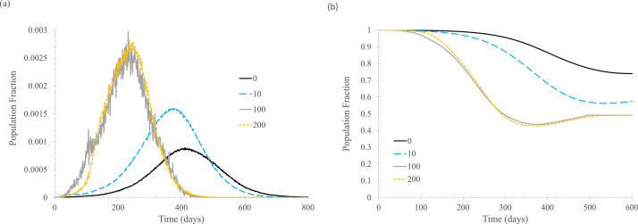
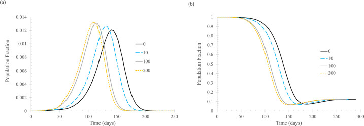
Figure 3 examines the timing to start contact tracing in terms of daily new cases of symptomatic infections. In the calculation, it is assumed that 50% of the newly infected can be tracked and will be isolated either when symptoms show up or 6 days after being infected, whichever comes first. Obviously, contact tracing should be started as early as practically possible, which is confirmed by the plots. Figure 3(A) shows that starting the process early, and in particular, starting contact tracing at the very beginning of the outbreak, can substantially reduce the daily number of new cases.

Fig 3.

The effect of when to start contact tracing in terms of daily new cases for symptomatic infections (N_start). In the simulation, f_tracked = 0.5, t_isolated = 6 days. (A) Daily new cases of symptomatic infections. (B) Fraction of susceptible population. Curve labels indicate the thresholds (of daily new symptomatically infected cases) at which contact tracing is initiated.

Comparing the curves in Figure 3 and the base case in Figure 2 indicates that it is never too late to start contact tracing. Even when it is started after the daily new cases of symptomatic infections reach 200 (out of 100,000 vertices in the entire network), contact tracing is still a meaningful NPI to mitigate the infection transmission.

Again, the modeling results show that the more effective contact tracing is at reducing daily new infection numbers, the more people will remain susceptible when the outbreak is over.

Finally, it is time to examine the effect of the percentage of newly infected that can be tagged and tracked from close contact with known cases of infection. In this study, an individual is counted as tagged and tracked only if that individual can be isolated later in the process. That is, the situation is complicated if an individual is successfully tagged and tracked by the public health authority and instructed to self-quarantine upon symptom appearance but fails to follow the order. Therefore, the percentage of tracked and isolated here represents the actual percentage of newly infected that is tracked and isolated when either symptoms show up or when the test result positively confirms the infection.

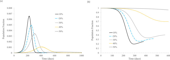
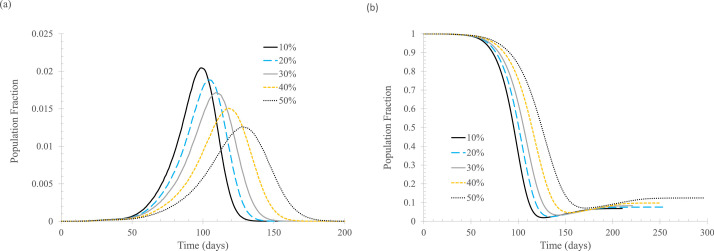
Figure 4 shows modeling results for the situation where contact tracing is implemented when the first case is known, and isolation of the tracked individual starts when symptoms appear or when the infection is confirmed through testing on the sixth day. As expected, tracking and isolating more infected people leads to lower daily new cases.

Fig 4.

The effect of percentage of newly infected, f_tracked. In the simulation, t_isolated = 6 days, N_start = 0. (A) Daily new cases of symptomatic infections. (B) Fraction of susceptible population. Curve labels indicate percentage quarantined for those being tagged and tracked.

A comparison between Figures 2 and 4 indicates that 50% isolation upon symptom onset alone is equivalent to 30% isolation when both symptom- and testing-based 6-day isolation are used. This is not surprising because the average incubation period is taken to be 5.8 days, that is, a half of the symptomatically infected will not show any symptoms in the first 6 days of infection, so the testing results will drive both the asymptomatically infected and presymptomatically infected into self-quarantine.

As the percentage of tracking and isolation increases, the effect of “flatten the curve” becomes “crush the virus.” As shown in Figure 4(B), although “crush the virus” is good for controlling the current outbreak, it leaves essentially the entire population susceptible for infection.

It is seen that contact tracing can be a very effective means to reduce the spread of the original strain of SARS-CoV-2. Tracking and isolating only 10% of infected people can make a meaningful difference. Therefore, every effort should be made to track as many potentially infected people as possible, including relaxing the definition of close contact, so that more infected people can be tracked and isolated. For example, many jurisdictions define close contact as within 6 feet for more than 15 minutes (or 30 minutes). This 6-foot rule is certainly not consistent with the findings for COVID-19 transmission in indoor environments.²⁴

It is worth noting that the virus spread reduction due to contact tracing in the present small-world network model is much more significant than that in the continuous deterministic models. For example, results^{25 , 26} from continuous deterministic models with comparable input parameters show a much less profound reduction of infection cases. A specific example²⁶ is with a 40% testing coverage, 1 day turnaround time of test results, and 60% contact tracing ratio, the peak infection number is reduced by only 50%, a level much lower than Figures 2 and 4 imply.

R₀ = 6

This subsection explores the effect of contact tracing on the behavior of infection transmission for a variant virus that has a much larger basic reproduction number than the original strain of SARS-CoV-2. It is now known that the delta variant, which was raging in the summer of 2021 in the United States, has a basic reproduction number around 6.^{16 , 17} This subsection presents modeling results obtained with R ₀ = 6. In the modeling, all other epidemiological parameters are assumed to be the same as in the previous section, and the infection profile is scaled up so that the sum of the daily infectivity rate is R ₀ = 6.

Figure 5 shows the differences between the no-contact-tracing base case and various approaches of isolation. It is seen that the progressively more stringent measures from depending on symptom onset alone to testing all tracked individuals have an increasing effect at lowering the daily peak infection numbers and at the same time, delaying the peaks, although the effect is not as appreciable as that for the case of R ₀ = 2.5.

Fig 5.

The effect of isolation time t_isolated. In the simulation, f_tracked = 0.5, N_start = 20, N_immune = 0. (A) Daily new cases of symptomatic infections. (B) Fraction of susceptible population. Curve labels are the same as those in Figure 2.

Unlike the original strain of SARS-CoV-2, when the delta variant starts to spread, the number of daily new cases does not start from 0, so the contact tracing is initiated with a nonzero daily new symptomatic cases. Thus, N _start is set to 20 in the simulation to obtain the results presented in Figure 5.

Figure 6 shows the effect of N _start. For completeness and for the purpose of examining the impact of starting contact tracing at the earliest possible stage, a case with N _start = 0 is included in the simulation. As expected, implementing contact tracing earlier in the process will bring better outcomes in terms of lowering and delaying the peak daily cases.

Fig 6.

The effect of when to start contact tracing in terms of daily new cases for symptomatic infections (N_start). In the simulation, f_tracked = 0.5, t_isolated = 6 days. (A) Daily new cases of symptomatic infections. (B) Fraction of susceptible population. Curve labels are the same as those in Figure 3.

Figure 7 shows that tracking and isolating a higher percentage of infected individuals can lower the peak daily cases and delay the occurrence of the peaks.

Fig 7.

The effect of percentage of newly infected, f_tracked. In the simulation, t_isolated = 6 days, N_start = 20, N_immune = 0. (A) Daily new cases of symptomatic infections. (B) Fraction of susceptible population. Curve labels are the same as those in Figure 4.

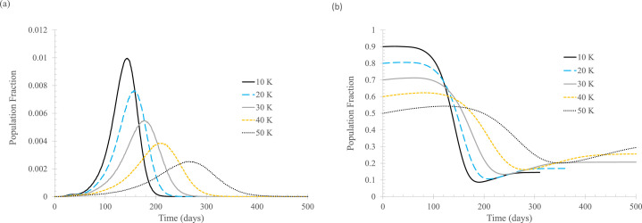
Finally, the fraction of the population with immunity at the beginning of a new outbreak is shown to have a significant effect. Figure 8 shows that with an increasing fraction of immune population, regardless of whether the immunity is gained from vaccination or previous infection, the peaks of daily new cases are lowered substantially, and these peaks occur much later in the process. An unexpected result is, as shown in Figure 8(B), the higher the initial percentage of the population that is susceptible, the lower the final percentage. This seems counterintuitive, but it makes sense: when the outbreak starts, the infection transmission is less widespread if a higher percentage of the population has immunity, so the infection is more likely to be extinguished.

Fig 8.

The effect of percentage of newly infected, N_immune. In the simulation, t_isolated = 6 days, N_start = 20, f_tracked = 0.5. (A) Daily new cases of symptomatic infections. (B) Fraction of susceptible population. Curve labels show the number of vertices that are immune to the infection at the beginning of the simulation.

The “crush the virus” phenomenon is absent for this example of high infectivity. The reason for its presence in the R ₀ = 2.5 case is as follows: when 50% of the new cases can be tracked and isolated, the effective reproduction number will be reduced to about 1.25. According to the continuous deterministic model, the infection is still sustainable at this low level of R ₀, but in the more realistic small-world network model, in 64 out of 100 realizations, the infection dies out on its own (that is, without any NPIs including contact tracing). Even with R ₀ = 2, simulation results show that in 25 out of 100 realizations, the infection ceases to continue after a very small number of infections. However, when R ₀ = 6, if the transmission is cut by half, the effective reproduction number is still about 3, higher than the R ₀ for the original strain of SARS-CoV-2.

Compared to the results obtained with R ₀ = 2.5, the effectiveness of contact tracing in bringing down the number of infections is not so great. Nonetheless, contact tracing is still quite a useful mitigation measure. Compare the curve for the nonmitigation base case in Figure 5(A) with those in Figure 7(A). It is seen that if 30% of the new cases can be tracked and isolated, the peak daily new cases can still be lowered from 2,171 to 1,715 (out of 100,000 vertices). Even if the isolation is solely based on symptom onset, the peak number is still reduced to 1,920 with a 30% tracking and isolation rate.

Discussion and conclusion

Among all NPIs to combat COVID-19, contact tracing is the least intrusive measure to the general public. As such, it should be utilized as the first choice for mitigation. It also works for other infectious diseases because it can reduce the spread of the disease in the broad public.

A small-world network model is used to study how contact tracing affects the infection transmission for COVID-19 and infectious diseases in general. It is better based than the conventional continuous deterministic mathematical models since it accounts for the essential characteristics of social networks. The continuous deterministic models tend to underestimate the efficacy of contact tracing, which may negatively affect public health officials allocating resources to this effort.

For the original strain of SARS-CoV-2, contact tracing alone can play a significant role in lowering and delaying the peak of daily new cases. Using symptom onset to decide entry to quarantine can help, but the benefit can be augmented greatly if test results are used to isolate asymptomatic and presymptomatic individuals. Another finding is that the sooner contact tracing is implemented, the better the outcome.

For the delta variant and other variants with high infectivity, contact tracing alone may not be a winning strategy, but it can certainly make a difference. Unlike the original strain of virus with a moderate basic reproduction number, starting contact tracing sooner seems to reduce the peak daily new cases only slightly. However, it can delay the peaks significantly, affording more time for medical professionals and public health authorities to develop pharmaceutical intervention measures.

To deal with outbreaks caused by variants of SARS-CoV-2, preexisting immunity (gained either from vaccination or previous infection) can play a vitally important role to reduce the number of daily new cases. Therefore, vaccinating the general public not only helps combat the current outbreak but also makes future outbreaks easier to deal with.

For both low and high infectivity diseases, increasing the percentage of tracked and isolated individuals among all the infected always leads to lowered numbers of new cases. This means that every effort should be made to enable more infected people to be tracked and isolated. This may include defining “close contact” more reasonably, making use of digital equipment such as smartphones to find individuals who may have close contact with those known to be infected, using test results to determine entry and exit to quarantine, providing support to the self-quarantined so they do not need to make trips to grocery stores and restaurants, maintaining daily contact with the self-quarantined, and providing support wherever and whenever necessary.

References

- 1.Baker RE, Park SW, Yang W, et al. The impact of COVID-19 nonpharmaceutical interventions on the future dynamics of endemic infections. Proc Natl Acad Sci U.S.A. 2020;117:30547–30553. doi: 10.1073/pnas.2013182117. [DOI] [PMC free article] [PubMed] [Google Scholar]
- 2.Bergwerk M, Gonen T, Lustig Y, et al. Covid-19 breakthrough infections in vaccinated health care workers. N Engl J Med. 2021;385:1474–1484. doi: 10.1056/NEJMoa2109072. [DOI] [PMC free article] [PubMed] [Google Scholar]
- 3.Giordano G, Blanchini F, Bruno R, et al. Modelling the COVID-19 epidemic and implementation of population-wide interventions in Italy. Nat Med. 2020;26:855–860. doi: 10.1038/s41591-020-0883-7. 2020. [DOI] [PMC free article] [PubMed] [Google Scholar]
- 4.Thompson RN. Epidemiological models are important tools for guiding COVID-19 interventions. BMC Med. 2020;18:152–155. doi: 10.1186/s12916-020-01628-4. [DOI] [PMC free article] [PubMed] [Google Scholar]
- 5.Brauer F, Castillo-Chavez C, Feng Z, et al. Springer; New York, NY: 2019. Mathematical Models in Epidemiology (vol. 69 of Texts in Applied Mathematics) [Google Scholar]
- 6.Pastor-Satorras R, Castellano C, Van Mieghem P, et al. Epidemic processes in complex networks. Rev Mod Phys. 2015;87:925–979. [Google Scholar]
- 7.Albert R, Barabási A. Statistical mechanics of complex networks. Rev Mod Phys. 2002;74:47–97. [Google Scholar]
- 8.Watts DJ, Strogatz SH. Collective dynamics of ‘small-world’ networks. Nature. 1998;394:440–442. doi: 10.1038/30918. [DOI] [PubMed] [Google Scholar]
- 9.Klemm K, Equiluz VM. Highly clustered scale-free network. Phys Rev E. 2002;65 doi: 10.1103/PhysRevE.65.036123. [DOI] [PubMed] [Google Scholar]
- 10.Broido AD, Clauset A. Scale-free Networks are Rare. Nat Commun. 2019;10:1017. doi: 10.1038/s41467-019-08746-5. [DOI] [PMC free article] [PubMed] [Google Scholar]
- 11.Newman MEJ, Watts DJ. Scaling and percolation in the small-world network model. Phys Rev E. 1999;60:7332–7342. doi: 10.1103/physreve.60.7332. [DOI] [PubMed] [Google Scholar]
- 12.Hansen CH, Michlmayr D, Gubbels SM, et al. Assessment of protection against reinfection with SARS-CoV-2 among 4 million PCR-tested individuals in Denmark in 2020: a population-level observational study. Lancet. 2021;397:1204–1212. doi: 10.1016/S0140-6736(21)00575-4. [DOI] [PMC free article] [PubMed] [Google Scholar]
- 13.Zhao S, Lin Q, Ran J, et al. Preliminary estimation of the basic reproduction number of Novel Coronavirus (2019-nCoV) in China, from 2019 to 2020: a data-driven analysis in the early phase of the outbreak. Int J Infect Dis. 2020;92:214–217. doi: 10.1016/j.ijid.2020.01.050. [DOI] [PMC free article] [PubMed] [Google Scholar]
- 14.D’Arienzo M, Coniglio A. Assessment of the SARS-CoV-2 basic reproduction number, R0, based on the early phase of COVID-19 outbreak in Italy. Biosaf Health. 2020;2:57–59. doi: 10.1016/j.bsheal.2020.03.004. [DOI] [PMC free article] [PubMed] [Google Scholar]
- 15.Weitz JS, Beckett SJ, Coenen AR, et al. Modeling shield immunity to reduce COVID-19 epidemic spread. Nat Med. 2020;26:849–854. doi: 10.1038/s41591-020-0895-3. [DOI] [PMC free article] [PubMed] [Google Scholar]
- 16.Xia F, Yang X, Cheke RA, Xiao Y. Quantifying competitive advantages of mutant strains in a population involving importation and mass vaccination rollout. Infect Dis Model. 2021;6:988–996. doi: 10.1016/j.idm.2021.08.001. 2006.2005.21258365. [DOI] [PMC free article] [PubMed] [Google Scholar]
- 17.del Rio C, Malani PN, Omer SB. Confronting the delta variant of SARS-CoV-2, summer 2021. JAMA. 2021;326:1001–1002. doi: 10.1001/jama.2021.14811. 2021.2006.2003.21258293. [DOI] [PubMed] [Google Scholar]
- 18.Oran DP, Topol EJ. Prevalence of asymptomatic SARS-CoV-2 infection: a narrative review. Ann Intern Med. 2020;173:362–367. doi: 10.7326/M20-3012. [DOI] [PMC free article] [PubMed] [Google Scholar]
- 19.Treibel TA, Manisty C, Burton M, et al. COVID-19: PCR screening of asymptomatic health-care workers at London hospital. Lancet. 2020;395:1608–1610. doi: 10.1016/S0140-6736(20)31100-4. [DOI] [PMC free article] [PubMed] [Google Scholar]
- 20.Wells CR, Townsend JP, Pandey A, et al. Optimal COVID-19 quarantine and testing strategies. Nat Commun. 2021;12:356. doi: 10.1038/s41467-020-20742-8. [DOI] [PMC free article] [PubMed] [Google Scholar]
- 21.He X, Lau EHY, Wu P, et al. Temporal dynamics in viral shedding and transmissibility of COVID-19. Nat Med. 2020;26:672–675. doi: 10.1038/s41591-020-0869-5. [DOI] [PubMed] [Google Scholar]
- 22.McAloon C, Collins A, Hunt K, et al. Incubation period of COVID-19: a rapid systematic review and meta-analysis of observational research. BMJ Open. 2020;10 doi: 10.1136/bmjopen-2020-039652. 2020. [DOI] [PMC free article] [PubMed] [Google Scholar]
- 23.Slifka MK, Gao L. Is presymptomatic spread a major contributor to COVID-19 transmission? Nat Med. 2020;26:1531–1533. doi: 10.1038/s41591-020-1046-6. [DOI] [PubMed] [Google Scholar]
- 24.Bazant MZ, Bush JWM. A guideline to limit indoor airborne transmission of COVID-19. Proc Natl Acad Sci. 2021;118 doi: 10.1073/pnas.2018995118. [DOI] [PMC free article] [PubMed] [Google Scholar]
- 25.Gardner BJ, Kilpatrick AM. Contact tracing efficiency, transmission heterogeneity, and accelerating COVID-19 epidemics. PLoS Comput Biol. 2021;17 doi: 10.1371/journal.pcbi.1009122. [DOI] [PMC free article] [PubMed] [Google Scholar]
- 26.Kim YJ, Koo PH. Effectiveness of testing and contact-tracing to counter COVID-19 pandemic: designed experiments of agent-based simulation. Healthcare. 2021;9:625. doi: 10.3390/healthcare9060625. [DOI] [PMC free article] [PubMed] [Google Scholar]