The distribution of COVID‐19–related risks

Abstract

We document two COVID‐19–related risks, viral risk and employment risk, and their distributions across the Canadian population. The measurement of viral risk is based on the VSE COVID‐19 Risk/Reward Assessment Tool, created to assist policy‐makers in determining the impacts of pandemic‐related economic shutdowns and re‐openings. Women are more concentrated in high‐viral‐transmission‐risk occupations, which is the source of their greater employment loss over the first part of the pandemic. They were also less likely to maintain contact with their former employers, reducing employment recovery rates. Low‐educated workers face the same viral risk rates as high‐educated workers but much higher employment losses. This is largely due to their lower likelihood of switching to working from home. For both women and the low‐educated, existing inequities in their occupational distributions and living situations have resulted in them bearing a disproportionate amount of the risk emerging from the pandemic. Assortative matching in couples has tended to exacerbate risk inequities.

1. Introduction

Risk is a pervasive element of the labour market. Workers face both exposure to illness and injury while at work and income risks associated with variation in wages, hours and job loss. Those risks are not equally distributed. For example, less‐educated workers have greater variability in employment over the business cycle (Hoynes et al. 2012, Delaney and Devereux 2019, Jaimovich and Siu 2009). And lower income workers may be compelled to go to work even when they are sick or when there is illness at their place of work because of their precarious income position—a point of interaction of the two types of risk. The COVID‐19 pandemic introduced substantially heightened risks of both types: it represents a new health risk that can be transmitted in close work arrangements and it required the shut‐down of whole industries, with associated job losses. Our goal in this paper is to characterize these two types of work‐related COVID‐19 risks with a focus on understanding how the risks vary across different groups of workers defined by gender, immigrant status, age and education. That is, we want to understand who is bearing the risks from COVID‐19 and how the health and job loss risks interact.

Workers can vary in their exposure to risks but the ultimate impact of that exposure depends on their ability to adjust to mitigate the risk. For COVID‐19–related health risks, one key way to adjust is to switch to working at home, where the worker is not exposed to risk of sickness from co‐workers. For job loss risk, labour hoarding by firms will reduce the risk for some workers. For others, they may be placed on some form of temporary lay‐off or put on an extended sick leave with or without pay. To the extent these adjustments are without pay, these forms of adjustment are less about helping workers with income loss during the firm downsizing than potentially allowing them to move more quickly back into work when the economy begins to recover. A third form of adjustment may come within households. If members of a household work in different industries with different levels of virus risk and job loss risk then the household can do some amount of self‐insuring, smoothing income to some degree. Access to these forms of adjustment is likely unequally distributed, implying that differential exposures to the initial risks could be exacerbated by differential ability to mitigate the risks if they do materialize. Moreover, an inability to adjust to mitigate the effects of job loss (because, e.g., of a lack of assets and savings) could lead to workers going to work sick, increasing their health risks and those of their co‐workers. We also examine these various forms of adjustment and how they differ by groups in society.

Carrying out this investigation requires a measure of the risk of acquiring the virus by workers at different workplaces. We use a measure we created to advise the federal and some provincial governments in the early part of the pandemic. In late March 2020, the director of the British Columbia Centre for Disease Control (BCCDC), Dr. Réka Gustafson, approached the Vancouver School of Economics (VSE) to analyze the economic impacts of the growing pandemic. The VSE formed several teams to examine different aspects of that impact, but a central component was to develop a means to characterize which parts of the economy were likely to be most affected. It is worth noting that at that point, there were no comprehensive surveys that included information on who was getting sick and where they worked. Shortly after starting this work, the VSE team became aware of researchers in Montréal and Halifax who were also working on this issue and a collaboration was undertaken between the two teams. A key part of the work concerned developing a list of characteristics of workers and their jobs that were most likely to put them at risk of contracting the virus. We worked with the BCCDC and its Quebec counterpart, the Institut national de santé publique du Québec (INSPQ), to create that list. The result was an index of riskiness (described in more detail below) that became the central element of the VSE COVID‐19 Risk/Reward Assessment Tool. We describe the tool in section 2 of the paper.

Several other researchers have developed measures of viral risk exposure. To the best of our knowledge, all other approaches have used only occupational workplace characteristics from the Occupational Information Network (O*NET hereafter) to conduct their analyses. For example, Dingel and Neiman (2020) focus on how likely it is that workers in a given occupation can work from home. They use a set of O*NET “work context” conditions (e.g., physical proximity, whether a worker spends the majority of the time on the job walking) and “work activities” conditions (e.g., handling and moving objects and operating vehicles), categorizing jobs as able to be done from home if any of the criteria do not apply. Similarly, a media outlet analysis by the The New York Times (Gamio 2020) and one by the Brookfield Institute (Vu and Malli 2020) consider the O*NET measures of physical proximity and exposure to disease and infection to rate occupations by COVID‐19 risk.

Our approach differs from other investigations in two important ways. First, we used input from public health experts to determine the set of characteristics that were most relevant for viral transmission. Second, our analysis includes characteristics of workers and their circumstances outside of work, not simply occupational characteristics from the O*NET. Part of what we learned from public health experts is that the spread of the SARS‐CoV‐2 virus depends not just on workplace conditions and interactions but also critically on non‐work conditions.1 This combination of workplace and worker information is unique. We were able to include worker characteristics because Statistics Canada provided remote access to non‐public use census and Labour Force Survey (LFS) data. We approached Statistics Canada early in our work regarding issues faced in developing useful measures for the BCCDC and the INSPQ on the basis of only public use microdata. Statistics Canada responded with remarkable speed and helpful assistance in working with the data.

The result is an interactive tool that includes our measure of viral transmission risk, the individual job and worker characteristics that underlie that measure, as well as measures of the economic importance of occupations. Our measures are available by four‐digit occupation and four‐digit sector level at the national and provincial levels.

Access to the administrative census data allows for further analysis. We are able to investigate who works in high‐risk occupations along dimensions such as gender, income/poverty and immigrant status. Combining census data with LFS data at the four‐digit occupation level, we examine what groups were most exposed to viral risk and what groups faced the largest job losses during the pandemic, and how these two risks interacted. In section 3, we describe the distribution of the virus risk, showing that women faced much higher exposure to this risk because of the occupations in which they are concentrated.

In section 4, we examine the risk of job loss, providing evidence for the claim that this is a “she‐cession” relative to earlier recession and also showing much larger job losses for the low‐educated and recent immigrants. We bring the two types of risk together in section 5, finding that high‐risk occupations experienced much higher rates of job loss and that extra job loss for women can be entirely explained by their concentration in high‐viral‐transmission‐risk occupations. In contrast, the low‐educated job loss happens across occupations, regardless of their level of virus risk. We follow up this analysis in section 6 with an examination of modes of adjustment to these risks. We find that women are further disadvantaged by having forms of work loss that involve lower ongoing connections with the firm. Using a rough counterfactual, we also find that the low‐educated experienced extra job loss because they were less able to make the switch to working from home. This may reflect different living arrangements. In this and in the concentration of women in virus exposed occupations, the pandemic has revealed and amplified inequities in society. The path forward involves not just income support but paying real attention to gender differences in occupations and to inequalities in living arrangements.

2. Risk/Reward Assessment Tool

The VSE COVID‐19 Risk/Reward Assessment Tool (VSE COVID‐19 Risk Tool hereafter) was created to help policy‐makers assess which occupations and sectors face the greatest risk of SARS‐CoV‐2 virus transmission. This was done in April of 2020 to provide guidance on the “re‐opening” of provincial economies and to aid in the monitoring of economic renormalization. The tool is also potentially useful in determining which sectors should be closed down in any subsequent waves of viral spread and where to target vaccine delivery to reduce work related viral risk.

The VSE COVID‐19 Risk Tool allows comparison of the viral transmission risks of occupational‐and‐sectoral activity relative to its importance to the economy. Our measure of viral transmission risk (VSE Risk Index hereafter)—the primary element of importance for this paper—is constructed at the four‐digit 2016 National Occupational Classification (NOC) code level, the finest level available in the census and LFS. The characteristics we use in the VSE Risk Index (detailed below) were determined in close consultation with public health experts at the BCCDC and INSPQ as those deemed most likely to expose workers to risk on the basis of what they were seeing in the population. They highlight specific concerns related both to the physical conditions at work and the living conditions for workers outside of the workplace. The analysis is performed separately for each province (except in the case of New Brunswick and Prince Edward Island, which were combined for data disclosure reasons) and for the Canadian economy as a whole. In this section, we provide details on the tool itself, the construction of the risk index and economic importance measures.

2.1. Interactive tool

In creating the VSE COVID‐19 Risk Tool, we followed three general design principles. First, the tool should be intuitive so that new users have minimal difficulty comparing the viral transmission risk and economic importance for the set of sectors and occupations that comprise each province's economy. Second, it should make disaggregated data available, allowing users to obtain a wide range of relevant sector, occupation and household characteristics. Third, the aggregated and disaggregated views into the data should be linked in a straightforward manner.

To fulfill the principle of being intuitive, the primary figure in the tool (see figure 1 below) is simply a scatterplot, with one of a set of measures of economic importance of a sector on the horizontal axis and the VSE Risk Index value on the vertical axis. Each point in the plot represents a sector‐occupation combination, scaled to indicate the occupation's within‐sector labour share. Users select different indicators of economic importance (all given at the three‐digit subsector level), including average sector employment in 2019, change in employment between February and April 2020, change in employment between February and April 2020 for jobs with wages that would place them in the lowest quartile of the wage distribution in 2019 and sectoral share of GDP.

FIGURE 1.

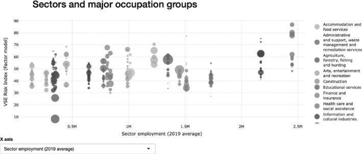
VSE COVID‐19 Risk Tool: Exhibit 1

NOTE: The online application can be accessed at https://COVID19.economics.ubc.ca/projects/project‐1/.

The table that follows the figure in the tool (see figure 2) fulfills the second principle of making disaggregated data available. Because these data represent the most granular occupation and subsector data available and include a large range of variables, there are thousands of rows and more than 30 columns to be displayed. To overcome this challenge, the tool uses a dynamic table: “pages” limits the number of rows displayed at once, “tabs” groups variables by type and filtering is available for all variables. Figure 2 shows a view of the table filtered to the “Retail trade” (code 44) sector and “Sales representatives and salesperson – wholesale and retail trade” occupation group (code 64). Third and finally, the figure and table are linked together. Users can click points in the figure to apply the relevant occupation and sector filters to the table to obtain detailed information on all of the disaggregated occupations within the larger occupation group.

FIGURE 2.

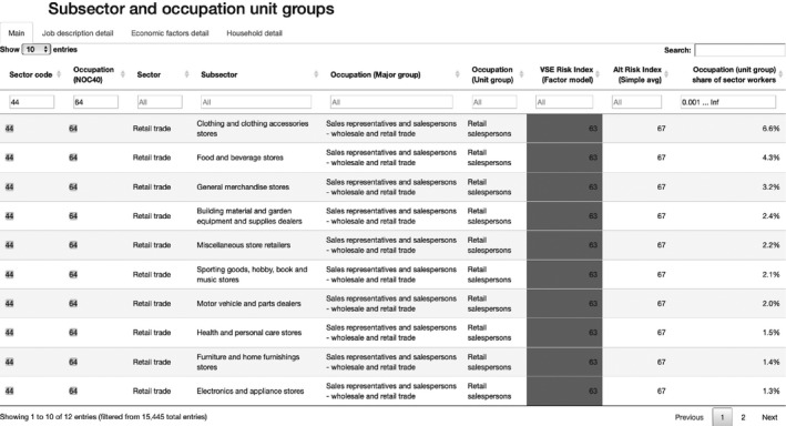
VSE COVID‐19 Risk Tool: Exhibit 2

NOTE: The online application can be accessed at https://COVID19.economics.ubc.ca/projects/project‐1/.

The online tool is an interactive application, which can be accessed at https://COVID19.economics.ubc.ca/projects/project‐1/. All of the code used to build the tool is available on the GitHub repository at www.github.com/pbaylis/vse‐risk‐tool, where more detail on its construction is available as well as instructions for running it on a user's own system.2

2.2. Viral transmission factors: Job characteristics

The VSE Risk Index is constructed using two principal data sources. The first source documents occupational work characteristics from the O*NET Version 24.2. This is a US‐based data source that provides information on approximately 300 characteristics of an occupation including skills required in performing job tasks and abilities possessed by workers in that occupation.

For our purposes, we focus on the “occupational requirements” domain of O*NET, detailing work activities, behaviours and physical work conditions. Under the “work context” and “work activities” categories of this domain, individuals employed in an occupation as well as experts on the occupation rate aspects of a job on a scale from 1 to 5 (the response scale is provided below). We use responses for:

1. Physical proximity: To what extent does this job require the worker to perform job tasks in close physical proximity to other people? [1 = Don't work near other people (i.e., beyond 100 ft.), 2 = Work with others but not closely (e.g., private office), 3 = Slightly close (e.g., shared office), 4 = Moderately close (at arm's length), 5 = Very close (near touching)].

2. Exposed to disease or infections: How often does this job require exposure to disease/infections? [1 = Never, 2 = Once a year or more but not every month, 3 = Once a month or more but not every week, 4 = Once a week or more but not every day, 5 = Every day].

3. Outdoors: How often does this job require working outdoors? We use both measures provided in the O*NET, working “exposed to weather” and “under cover” [same scale as exposed to disease or infections].

4. Contact with others: How much does this job require the worker to be in contact with others (face‐to‐face, by telephone, or otherwise) in order to perform it? [1 = No contact with others, 2 = Occasional contact with others, 3 = Contact with others about half the time, 4 = Contact with others most of the time, 5 = Constant contact with others].

5. Performing for or working directly with the public: Performing for people or dealing directly with the public. [1 = Not important at all, 2 = Somewhat important, 3 = Important, 4 = Very important, 5 = Extremely important].

The O*NET provides information for 974 occupations coded according to the Standard Occupational Classification (O*NET‐SOC) system. We use a crosswalk developed by Marc Frenette at Statistics Canada (StatCan) to map these into the NOC 2016, which has approximately 500 occupation unit groups at the finest four‐digit level of granularity.3

2.3. Viral transmission factors: Worker characteristics

The second important source of information is the 2016 Census of Population, from which we obtained worker characteristics by occupation. Because we wanted to examine those characteristics at the narrowest (four‐digit) occupation level, the public use version of the census was not sufficient for our purposes. Because of pandemic‐related closures, the confidential files could not be accessed via StatCan's regional data centres (RDCs). We approached StatCan and were given very rapid remote access to the data we required, in walled‐off parts of their servers. StatCan adapted RDC protocols so that we could access the confidential data and have our research results vetted to make sure confidentiality requirements were met. Because SARS‐CoV‐2 transmission depends importantly on factors outside of the workplace, characteristics of workers obtained from the census play an important role in our measurement of viral transmission risk. The inclusion of these characteristics is unique to our analysis. The variables listed below correspond to the proportion of workers employed in a four‐digit NOC occupation code that have a certain characteristic:

1. Works from home: Job is located in the same building as their place of residence, lives and work on the same farm or spends most of their work week working at home.

2. Public transit: Takes public transit, including bus, subway/elevated rail, light rail/streetcar/commuter train and passenger ferry, but excluding carpooling, as the main mode of commuting to work.

3. Lives with health worker: Lives with someone who works in ambulatory healthcare services, hospitals or nursing and residential care facilities.

4. Crowded dwelling: Lives in an “unsuitable dwelling,” where a dwelling is deemed unsuitable if it has too few bedrooms for the size and composition of the household, according to the National Occupancy Standard.

Again, the characteristics listed in subsections 2.2 and 2.3 were chosen in collaboration with public health officials as those most relevant to viral transmission risk.

2.4. VSE Risk Index

Currently available data do not allow us to directly observe SARS‐CoV‐2 transmission risk. Hence, a key issue is determining how to aggregate the various occupational and worker characteristics listed above into a single risk index. To the extent that these characteristic measures vary together, they capture changes in an underlying or latent risk of transmission. We exploit this intuition in the construction of the VSE Risk Index.

We do so via factor analysis, in which a set of observed variables are portrayed as combinations of an underlying subset of unobserved latent variables called “factors.” The coefficients associating factors to each of the observed variables are called “factor loadings.” For the VSE Risk Index, we focus on the first factor, which involves finding the combination of measures that accounts for the largest proportion of their covariance.4 The first factor represents a common element in the set of characteristics listed above; in that sense, it is a natural candidate for the VSE Risk Index. To facilitate interpretation as an index, we normalize this factor to [0, 100] scale.

The factor analysis delivers intuitive results with respect to the ranking of occupations by viral transmission risk. Health‐related occupations uniformly occupy the top of the distribution. At greatest risk are dentists; general practitioners and family physicians; and respiratory therapists, clinical perfusionists and cardiopulmonary technologists, with VSE Risk Index scores of 100, 94 and 91, respectively. The riskiest non‐health occupations are Pursers and flight attendants and Food service supervisors, largely because of their very close physical proximity and constant contact with others. At the other extreme, occupations with the lowest risk scores are chain saw and skidder operators; managers in agriculture; and conductors, composers and arrangers, with VSE Risk Index scores of 0, 7 and 10, respectively. For the sake of brevity, we refer readers to the VSE COVID‐19 Risk Tool for details regarding other occupations and associated sector risk measures, at https://COVID19.economics.ubc.ca/projects/project‐1/.

2.5. Economic importance variables

In addition to the VSE Risk Index, the VSE COVID‐19 Risk Tool provides several measures of the relative economic importance of specific sectors. These measures are constructed at the three‐digit (or “subsector”) categorization level in the North American Industry Classification System (NAICS), Canada 2017 Version 3.0. In terms of importance, sectors can be compared along three dimensions.

The first is simply the size of the sector, in terms of employment or GDP. The second is in terms of sectoral employment losses between February and April 2020, which varied widely across sectors. For instance at the national level, employment was essentially halved in Accommodation and Food Services, while Finance and Insurance saw very little change in employment. The tool also allows users to focus on job loss in the bottom quartile of the wage distribution. As is well known, the effects of recessions are disproportionately borne by those most economically disadvantaged; the unprecedented shutdown in this episode is no exception (as discussed below). Finally, sectors can be organized by a measure of network centrality: how essential they are to the functioning of all other sectors of the economy, in terms of intersectoral input–output linkages.

2.6. The tool's role in public policy

The VSE COVID‐19 Risk Tool was created to aid policy‐makers assess the risks and benefits of re‐starting various sectors of the economy and, as needed, re‐introduction of closures or restrictions in subsequent waves of virus transmission. Because the VSE Risk Index is measured at the occupational level, the tool also allows policy‐makers to identify, within sectors, jobs or areas that require particular attention as economic activity renormalizes.

To date, results have been shared in British Columbia with senior officials within the premier's office, the ministries of Finance, Health and Social Policy and Poverty Reduction and the BCCDC and with WorkSafe BC, the agency responsible for workplace injury and illness that is overseeing safety in the province's Restart plan. In Quebec, results have been shared with the finance ministry and the INSPQ.

At the federal level, the VSE COVID‐19 Risk Tool has been shared with senior officials at Health Canada, Public Health Agency of Canada, Public Safety Canada, the Canadian Centre for Occupational Health and Safety, Statistics Canada, the Bank of Canada and numerous federal ministries. The Labour Market Information Council (LMIC) generously supported our research to extend the analysis beyond BC and Quebec to all provinces and the Canadian economy at the national level. Through the LMIC, the VSE COVID‐19 Risk Tool has been shared with its constituent ministries (those principally of labour and skills development) from each province and territory. In addition, the tool has been shared with public health officials from each province and territory.

The VSE COVID‐19 Risk Tool is also potentially useful in prioritizing vaccinations, especially given short‐run supply constraints. Prioritization of the elderly and those residing and working in long‐term care facilities indicates the public health rationale for prioritizing those at highest risk of infection. The VSE Risk Index is a measure of viral transmission risk across occupations and therefore provides additional information that can be incorporated into such decisions. For instance, while front‐line workers in hospital settings are obvious candidates, the VSE Risk Index indicates that other health‐care workers, such as dentists and dental hygienists, face important occupational risk. Finally, the Tool also provides sectoral measures of economic importance that may be worthy of prioritization. For instance, Green et al. (2020) extends the network centrality analysis discussed above; they find that in‐person K–12 schooling is of critical importance in “freeing up” time of parents with school‐aged children to be supplied as labour to all sectors of the economy. This indicates the importance of elementary and secondary school teachers in such considerations.

3. Who bears the risk of viral transmission?

We begin by using the VSE Risk Index and its component series to investigate who is most exposed to workplace viral risk from COVID‐19. We do this at the four‐digit occupational level, asking whether certain demographic and skill groups are disproportionately employed in occupations with high‐viral‐transmission‐risk scores.

In figure 3, we present results from regressing the VSE Risk Index on the proportion of workers in a given occupation who are female, belong to different age groups, are recent immigrants (i.e., immigrated to Canada in the previous 10 years), have lower educational attainment (high school or less) and live in low‐income households (as defined by the after‐tax Market Basket Measure poverty line). These are characteristics that may be associated with risk but are not included in the construction of the risk index. Results in figure 3, panel A, come from bivariate regressions, with the exception of the age variables, which are included together in a single regression (with 15‐ to 24‐year‐olds as the excluded group). Results in figure 3, panel B, come from a (multivariate) regression of the VSE Risk Index on the full set of variables.

FIGURE 3.

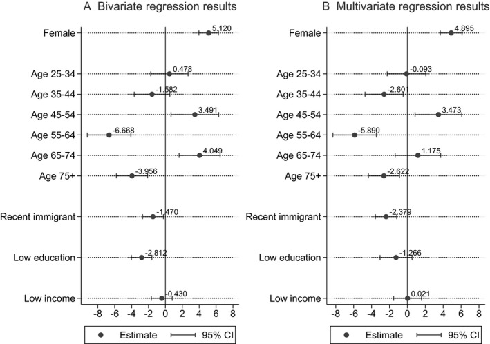
Regression of risk on occupation‐level characteristics: All occupations

NOTES: Point estimates and 95% confidence intervals of VSE Risk Index regressed on demographic characteristics of four‐digit NOC occupations. Panel A presents bivariate regression results. Panel B presents multivariate results. See text for details.

Our principle finding is that gender is an important correlate of viral transmission risk: a one‐standard‐deviation increase in the proportion of workers who are female is associated with a 5.12 point increase in the average risk index, or approximately one third of a standard deviation.5 By comparison, risk is only modestly (and negatively) associated with the prevalence of immigrants across both specifications. Risk displays a negative relationship with low education only in the bivariate case and is not associated with the proportion of individuals from low‐income families. Age bears a non‐linear relationship to viral risk, with occupations with a high concentration of workers aged 45 to 54 being relatively high risk and those with more workers in the 55‐ to 64‐year‐old range being relatively low risk.

In figure 4, we unpack the patterns in figure 3 by presenting the relationship between the demographic and skill factors and the different components of the risk index. Each entry in a line shows the marginal effect of the corresponding factor (e.g., proportion of workers who are female) in a multivariate regression of the risk component on the full set of factors. The results are expressed in fractions of a standard deviation of the risk component. Women tend to work in occupations with much greater viral transmission risk with respect to all O*NET characteristics compared with men; this is indicated in the left‐most figure in the first row of figure 4 (note that “working outdoors” is associated with lower risk). In addition, while female‐dominated jobs feature a lower proportion of workers that cohabitate with a healthcare worker, they are more associated with all other census‐based characteristics included in the VSE Risk Index. Thus, female workers have both home and work characteristics associated with greater virus risk.

FIGURE 4.

Regression of risk factors on occupation‐level characteristics: All occupations

NOTES: Point estimates and 95% confidence intervals of risk components regressed on demographic characteristics of four‐digit NOC occupations. Results come from multivariate regressions of each risk component on the set of demographic characteristics. Each panel presents the marginal effect of the corresponding characteristic in each of these regressions.

By contrast, the weak relationship between immigrant status and overall viral risk shown in figure 3 is the result of offsetting occupational and worker characteristics. Immigrant‐dominated occupations tend to have lower direct contact with others, especially the public (lowering their viral transmission risk), but their workers have a greater tendency to live in crowded dwellings and to take public transit to work (increasing their risk). This is important given recent concerns that racialized populations face greater risk from the virus (Gross et al. 2020, Millett et al. 2020, Price‐Haywood et al. 2020). Our results indicate that this is not true in terms of workplace arrangements but is true in terms of living conditions.6

For occupations with high proportions of low‐educated and low‐income workers, there is no consistent pattern in the set of occupational characteristics nor in the home characteristics of workers.

Figure 3 indicates that occupations with a high proportion of 45‐ to 54‐year‐old workers are associated with greater viral transmission risk, while those with many 55‐ to 64‐year‐olds are lower risk. The corresponding panels in figure 4 show that these two age groups are essentially mirror images in terms of workplace characteristics, with 45‐ to 54‐year‐olds being in jobs with greater proximity, disease risk, contact with others (particularly the public) and 55‐ to 64‐year‐olds being the opposite. We do not have an explanation for these differences but note that they hold up even when controlling for immigrant status, education level and low‐income status.7

4. Who bears the risk of job loss?

In this section, we investigate how the loss of employment has been distributed across workers in the Canadian economy, using monthly data from the LFS from January to June 2020. As has been widely reported, employment losses during the initial stages of the pandemic shutdown are far‐and‐away the largest recorded during the postwar era (Lemieux et al. 2020). Employment has since rebounded but is still well below pre‐COVID‐19 levels. In figure 5, we show employment losses in both absolute and percentage changes, relative to February 2020 employment levels, for all workers, as well as separately for female, immigrant and low‐educated workers.

FIGURE 5.

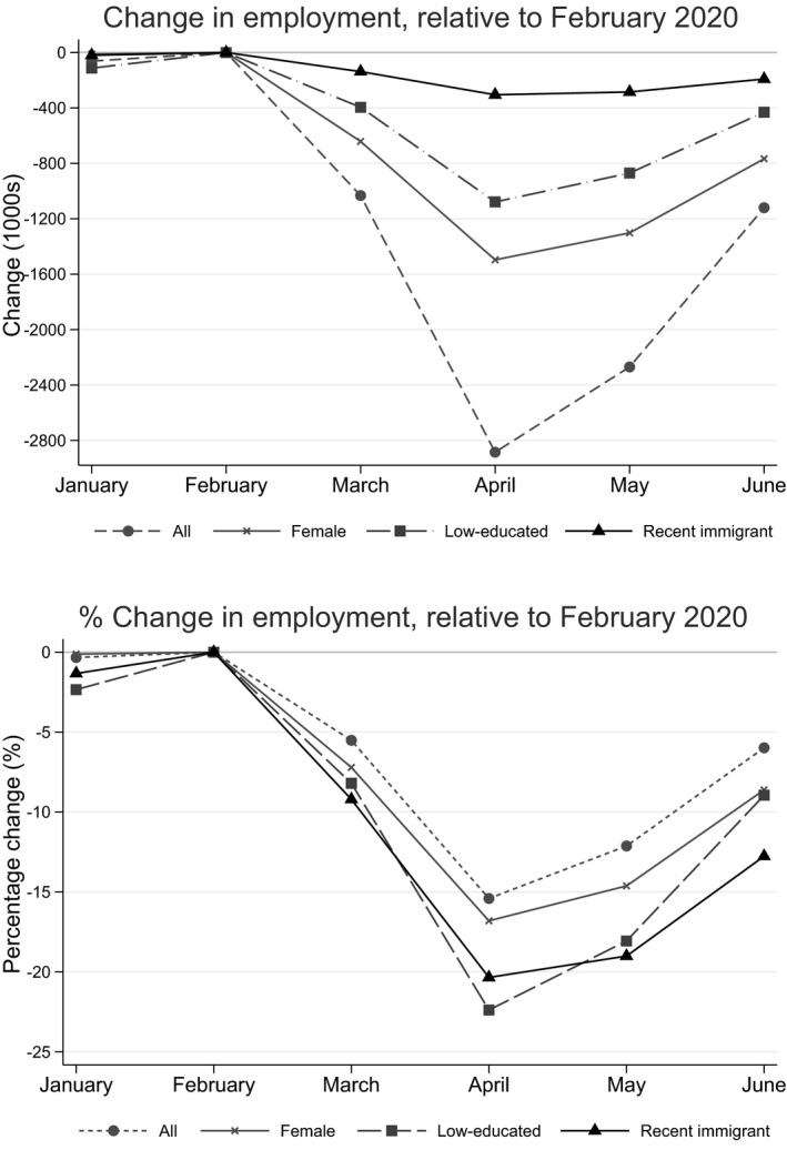
Employment loss, for all and by demographics

NOTES: Changes in employment are computed relative to February and percent changes are normalized using the February level of employment. Employment incorporates both being at work and being absent from work.

To provide context, in the left panel of figure 6, we plot percentage changes in employment for all workers and our demographic sub‐groups for the 2008/2009 recession. In particular, we plot percentage changes relative to September 2008 for the period from September 2008 through April 2009 (from one definition of the start of the recession through to its trough). The patterns reflect the standard pattern that recessions are most harmful for the most economically marginalized: lower‐educated and immigrant workers (see Jaimovich and Siu 2020). Moreover, the 2008/2009 recession reflects the standard finding that women tend to face smaller job losses than men in recessions.

FIGURE 6.

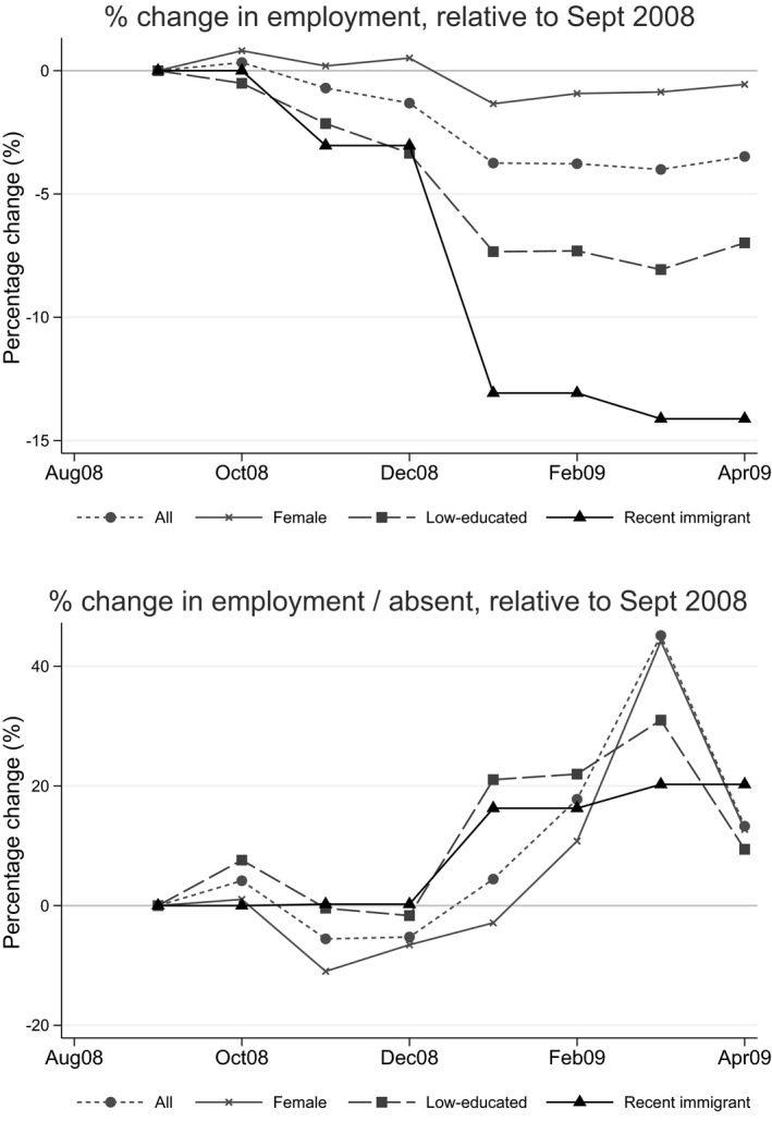
Employment loss, for all and by demographics, 2008 recession

NOTES: Percent changes are normalized using the September 2008 level of employment. Employment incorporates both being at work and being absent from work.

The 2020 recession shown in figure 5 also included larger negative employments effect for immigrant and lower‐educated workers. This is particularly evident in the percentage changes shown on the right, in panel B. While total employment fell by 15.4% (for all workers) between February and April, it fell by 22.4% for the less‐educated (those with high school attainment or less) and by 20.4% for recent immigrants (landed immigrants, arrived in Canada between 2010 and 2020 inclusively). A similar discrepancy is evident, particularly for immigrants, when we include the subsequent partial recovery, April to June. By comparison, in the 2008/2009 recession, immigrant employment followed the same pattern of an initial sharp drop followed by a relatively anemic recovery, but the drop amounted to a smaller, 15%, decline. For the low‐educated, similarly, employment losses were larger than for the higher‐educated but, again, much smaller than in the 2020 recession (an 8% decline compared with over 20% in the current recession).

The most striking characteristic of the current recession is that job loss for female workers has also been disproportionately high. In the 2008/2009 recession, female job loss was relatively negligible, with the male decline being over 6% greater. This is also true in earlier recessions, arising because of the greater concentration of male workers in both routine production occupations and in cyclically sensitive construction occupations. However, in the current “pandemic” recession, the pattern has been flipped: women have borne the disproportionate share of employment loss. Total employment fell by 15.4% (for all workers) between February and April and by 6.0% between February and June. By contrast, female employment fell by 16.8% and by 8.6% over those same time periods. Put differently, women have accounted for 68.5% of total job loss since February, despite accounting for 47.6% of employment averaged over January and February of 2020. Job loss effects are certainly more evident for low‐educated and immigrant workers; however, there is reason to call this a “she‐cession” when viewed in comparison to earlier recessions.8 Thus, women bear a greater burden from both types of risk created by the pandemic: risk of contracting the virus at work and risk of job loss. We investigate the relationship between these two risks in the next section.

The employment numbers in figure 5 correspond to the standard Statistics Canada definition of employment, including everyone who reports that they are employed during the LFS survey week. However, employment can have different forms and the LFS also asks respondents whether they are employed and present at work, employed and absent from work for the whole week and, if absent, whether they were being paid. In figure 7, we show changes in the numbers of individuals who report being employed but absent from work for the survey week. We provide numbers for the 2008/2009 recession for comparison in the right panel of figure 6.

FIGURE 7.

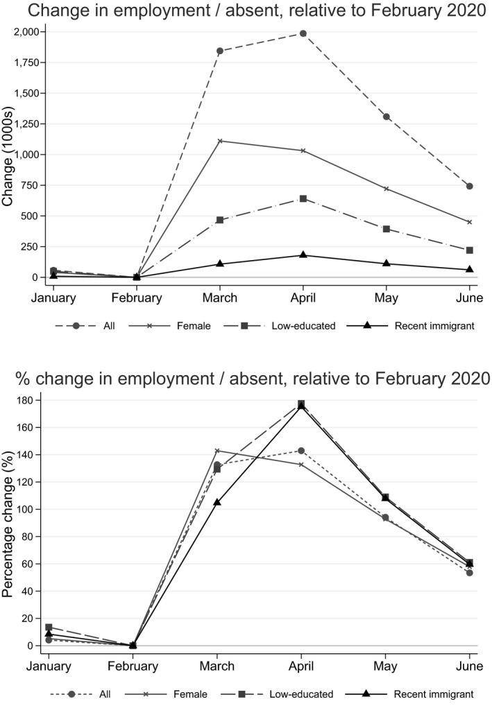
Increase in being employed but absent, for all and by demographics

NOTE: Changes in employment are computed relative to February and percent changes are normalized using the February level of employment.

Comparison to the left panel of figure 5 affords an understanding of the magnitude of work disruption. From February to April, over 2.8 million jobs were lost. Figure 7 indicates the extent to which that understates the amount of “work lost”: during that same time period, an additional 2.0 million individuals were employed but absent from work, amounting to almost $\frac{3}{4}$'s (71%) of job loss. From April to June there was a reduction in the number who were employed/absent, mirroring the recovery in employment, but still remained far from pre‐COVID‐19 values.

Comparing figure 7 with the right panel of figure 6, we see that the use of the employed but absent state has been much greater in the 2020 recession than in the previous one. For all workers combined, the employed but absent state increased in size by about 40% in the 2008/2009 recession but by 140% in the 2020 recession. This likely reflects the nature of the 2020 recession as one that was purposefully induced, with firms unsure about when they could re‐open and, so, interested in maintaining an attachment to their workers. Gender effects again switch signs between the two recessions, with women having smaller increases (or larger decreases) in their probability of being employed but absent in the 2008/2009 recession and slightly larger increases in probability in the first part of the 2020 recession, but the differences are small. The effects for the low‐educated and immigrants also switch signs, with them being pushed less into the employed‐but‐absent state in the later part of the 2008/2009 recession than higher‐educated and non‐immigrant workers but more into that state in the most recent months of this recession.

A key difference between the COVID‐19 recession and earlier recessions is the likely importance of labour supply side factors in the employment patterns we have shown here. By and large, recessions are seen as labour demand side phenomena: for reasons that are only partially understood and much debated, there is a co‐ordinated decline in demand for workers on the part of firms. With COVID‐19, these demand reductions also existed—in part because of public health orders shutting down certain sectors and in part because consumers were cautious about engaging with firms in person—but there have also been supply side factors. In particular, schools and daycares were closed through much of the end of the 2019/2020 school year. This resulted in some parents having to withdraw from work to take care of their children. The results in Green et al. (2020), which show that the K–12 education sector accounts for as much as 11.5% of GDP if one takes account of its role in enabling parents to go to work, imply that this supply‐side channel could have been substantial. In addition, some workers likely chose not to continue working out of concern about contracting COVID‐19 in their workplaces. With the data we have, we have no way to disentangle the effects of these two forces in driving the decline in employment through April of 2020. In May and June of 2020, only Quebec fully re‐opened its schools, and even there, it was only schools outside of Montréal. Given that, it seems likely that the strong rebound in May and June of 2020 shown in figure 5 was mainly a demand side phenomenon. The fact that the rebound was somewhat slower for women than men may fit with this as well. In future work, it would be interesting to use differences by gender and by jurisdiction (in terms of school openings) to identify the relative importance of the demand and supply channels. It would also be interesting to try to identify the effects of major government transfers, with transfers like the Canada Emergency Response Benefit (CERB) likely being expected to reduced labour supply while the Canada Emergency Wage Subsidy might have maintained employment links at a higher level than would otherwise have occurred.

5. The relationship between employment and viral transmission risks

Viral risk and employment risk are not independent. Viral risk leads to job losses through multiple channels, such as governments shutting down or restricting non‐essential businesses—hitting especially retail; manufacturing, business services and entertainment; and the hospitality industry—businesses closing out of precautionary reasons for employees and customers or being unable to meet newly introduced requirements on safe working conditions, or due to a decline in demand for their goods or services produced.9 Some of the job losses also stem from voluntary resignation or decrease of labour supply, for reasons such as caring of elderly and children at home. From the public health perspective of minimizing viral transmission, policy would prioritize shutting down sectors where viral risk is greatest. To the extent this is true, the two risks may interact and exacerbate negative impacts. As discussed in section 3, women face greater viral risk and, from the numbers in section 4, also experienced greater employment loss.

We take a first step at assessing these interactions in figure 8. In both panels, employment losses are displayed separately for health‐ and non‐health‐related occupations.10 Non‐health occupations are further disaggregated by (2019 employment weighted) terciles of the VSE Risk Index. We do this because health‐related occupations—while associated with the highest levels of viral transmission risk according to our methodology—exhibited very different employment dynamics compared with other high‐viral‐transmission‐risk occupations because of their obvious essential service function.

FIGURE 8.

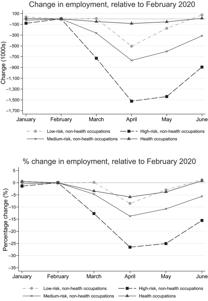
Employment loss by VSE Risk Index

NOTES: Changes in employment are computed relative to February and percent changes are normalized using the February level of employment. Non‐health occupations are classified into three equal categories (low/medium/high) on the basis of their VSE Risk Index, weighted by the share of 2019 employment in a given four‐digit occupation. Employment incorporates both being at work and being absent from work.

Figure 8 makes it clear that job loss was not experienced evenly across the distribution of viral transmission risk: occupations with high‐viral‐transmission‐risk scores lost many more jobs than lower‐risk occupations. Relative to February, top tercile occupations lost about 1.5 million jobs, compared with around 500,000 jobs for bottom tercile occupations. By June, employment in low‐risk occupations exceeded February levels, whereas high‐risk occupations were still well short. In percentage terms, by June, the high‐risk occupations were still 15.5% below their February employment levels, medium risk occupations were 5.6% below, while both low‐risk and health occupations were above their February levels. In comparison, figure 9 shows employment changes for the 2008/2009 recession broken down by the same COVID‐19 viral risk categories. In that recession, what would years later turn out to be the high‐viral‐transmission‐risk occupations actually experienced employment increases and it was the low‐risk occupations that had the greatest employment declines. This finding validates the VSE Risk Index because one would expect occupations ranked as high risk to be more likely to be shut down when the virus is present but not necessarily when it is not. Interestingly, health occupations were relatively “recession‐proof” in both recessions.

FIGURE 9.

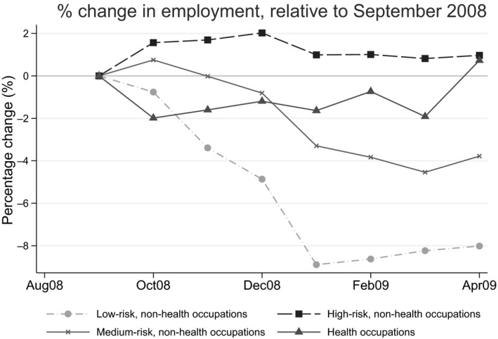
Employment loss, by virus risk categories, 2008 recession

NOTES: Percent changes are normalized using the September 2008 level of employment. Non‐health occupations are classified into three equal categories (low/medium/high) on the basis of their VSE Risk Index, weighted by the share of 2019 employment in a given four‐digit occupation. Employment incorporates both being at work and being absent from work.

Figure 10 presents employment numbers by viral risk separately for our main demographic groups. Here, the interaction of viral risk and job loss amplifies effects for disadvantaged groups. For the low‐educated, employment in high‐risk occupations dropped by 34% between February and April and recovered to only about 20% below its February level by June. For immigrants, the loss is more severe, with June employment still almost 30% below its February level. For immigrants, June employment in health occupations is well below its February level, though overall employment is slightly above. For women, the employment loss in high‐risk occupations is slightly greater than that displayed in figure 8; employment loss in middle risk occupations is large relative to men by the end of our period. Note that the non‐health occupation terciles are defined for the overall population and from section 3, women are overrepresented in higher‐risk occupations. This leads to the higher job losses for women discussed above in section 4.

FIGURE 10.

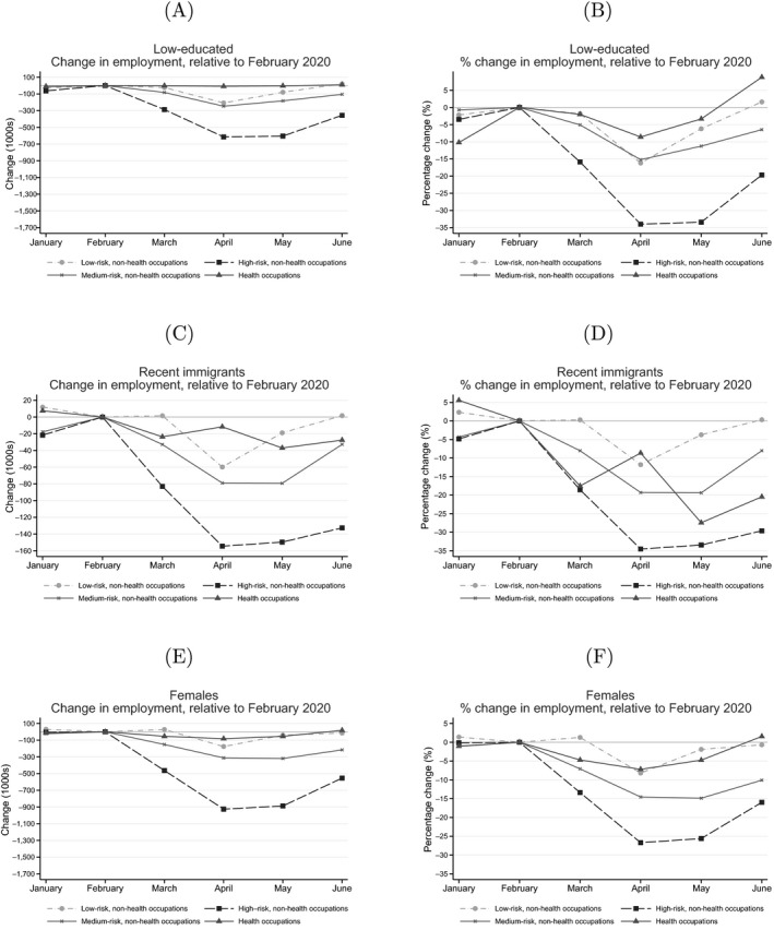
Detailed employment loss by VSE Risk Index and demographics.

NOTES: Changes in employment are computed relative to February and percent changes are normalized using the February level of employment. Non‐health occupations are classified into three equal categories (low/medium/high) on the basis of their VSE Risk Index, weighted by the share of 2019 employment in a given four‐digit occupation. Employment incorporates both being at work and being absent from work.

Tables 1 and 2 present regression analysis to further illustrate that job loss was not experienced evenly across the distribution of viral transmission risk. We do so at the granular, four‐digit occupation level (as opposed to risk terciles). Table 1 presents results for employment change in non‐health occupations between February and April; table 2 presents results for April to June. In both tables, absent workers are excluded from the definition of employment and change in employment is expressed relative to occupational employment observed in February.

TABLE 1.

Regression of change in employed, at work (February–April, relative to February) on VSE Risk Index and components

Independent variable:	Occupational employment change
	(1)	(2)	(3)	(4)	(5)	(6)	(7)
Std. VSE Risk Index	−0.145**				−0.122**		−0.118**
	(0.024)				(0.020)		(0.018)
Std. O*NET measures
Proximity		−0.172**	−0.129**	−0.146**		−0.144**
		(0.023)	(0.027)	(0.028)		(0.028)
Disease		0.047	0.039	0.024		0.030
		(0.035)	(0.027)	(0.023)		(0.029)
Outdoor		$0.{041}^{+}$	0.048	$0.{061}^{+}$		0.055
		(0.020)	(0.025)	(0.026)		(0.031)
Contact		0.081**	0.031	0.035		0.037
		(0.022)	(0.023)	(0.025)		(0.025)
Public		−0.084*	$-0.{060}^{+}$	−0.044		−0.042
		(0.025)	(0.025)	(0.024)		(0.023)
Std. census share measures
Live with health worker			−0.020	−0.016		−0.024
			(0.033)	(0.031)		(0.033)
Unsuitable dwelling			−0.075**	−0.009		−0.014
			(0.021)	(0.025)		(0.041)
Public transit for work			$0.{035}^{+}$	0.014		0.015
			(0.016)	(0.018)		(0.018)
Working from home			−0.015	−0.015		−0.015
			(0.013)	(0.015)		(0.015)
Low education				−0.081*	−0.096**	$-0.{077}^{+}$	−0.094**
				(0.026)	(0.017)	(0.030)	(0.018)
Female						−0.013	−0.007
						(0.031)	(0.018)
Recent immigrant						0.005	−0.015
						(0.033)	(0.013)
Constant	−0.277**	−0.291**	−0.272**	−0.277**	−0.259**	−0.277**	−0.255**
	(0.023)	(0.023)	(0.021)	(0.021)	(0.017)	(0.021)	(0.019)
Observations	458	458	458	458	458	458	458

Table shows the estimated linear regression coefficients of the change in employment on standardized measures of viral transmission risk, where one observation corresponds to a four‐digit occupation. Standard errors are in parentheses and are clustered at the two‐digit occupation level. Statistical significance is denoted by ** at the 1% level, * at the 5% level and at the 10% level. Health occupations are excluded from the sample. Regressions are weighted by the share of 2019 employment in a given four‐digit occupation.

TABLE 2.

Regression of change in employed, at work (April–June, relative to February) on VSE Risk Index and components

Independent variable:	Occupational employment change
	(1)	(2)	(3)	(4)	(5)	(6)	(7)
Std. VSE Risk Index	0.016				−0.009		0.008
	(0.027)				(0.031)		(0.032)
Std. O*NET measures
Proximity		0.075*	0.032	0.046		0.025
		(0.023)	(0.032)	(0.032)		(0.044)
Disease		$-0.{069}^{+}$	−0.060*	$-0.{048}^{+}$		−0.066
		(0.027)	(0.019)	(0.018)		(0.039)
Outdoor		0.057	0.057	0.047		0.056
		(0.042)	(0.056)	(0.055)		(0.070)
Contact		−0.083*	−0.048	−0.051		−0.046
		(0.029)	(0.027)	(0.028)		(0.031)
Public		0.048	0.029	0.017		−0.0022
		(0.035)	(0.033)	(0.033)		(0.024)
Std. census share measures
Live with health worker			0.003	0.000		0.003
			(0.023)	(0.023)		(0.034)
Unsuitable dwelling			0.060**	0.006		0.108
			(0.016)	(0.021)		(0.065)
Public transit for work			−0.0261	−0.009		−0.006
			(0.017)	(0.019)		(0.021)
Working from home			−0.013	−0.013		−0.007
			(0.018)	(0.020)		(0.021)
Low education				0.066*	0.104*	0.010	0.103*
				(0.023)	(0.031)	(0.037)	(0.034)
Female						0.017	$-0.{035}^{+}$
						(0.046)	(0.013)
Recent immigrant						−0.094	−0.032
						(0.054)	(0.029)
Constant	0.193**	0.206**	0.190**	0.194**	0.174**	0.189**	0.188**
	(0.026)	(0.020)	(0.017)	(0.016)	(0.019)	(0.017)	(0.021)
Observations	458	458	458	458	458	458	458

Table shows the estimated linear regression coefficients of the change in employment on standardized measures of viral transmission risk, where one observation corresponds to a four‐digit occupation. Standard errors are in parentheses and are clustered at the two‐digit occupation level. Statistical significance is denoted by ** at the 1% level, * at the 5% level and at the 10% level. Health occupations are excluded from the sample. Regressions are weighted by the share of 2019 employment in a given four‐digit occupation.

The first column considers the bivariate relationship between occupational employment change and the VSE Risk Index and reinforces the findings of figure 8. Table 1 indicates a much larger drop in employment for higher‐risk occupations between February and April; table 2 indicates no significant difference in employment recovery by VSE Risk Index from April to June. In combination with the difference in baseline employment changes, as captured by the estimated regression constants, riskier occupations have exhibited larger job losses during the pandemic to date, February to June.

Columns 2 and 3 show the marginal effects of the various characteristics included in the VSE Risk Index. In column (2) of table 1, we regress changes in employment on occupational characteristics alone. We view this as informative given the emphasis on O*NET characteristics in other work (see, e.g., Dingel and Neiman 2020). The coefficient signs, and the relative size and significance, accords with intuition. In particular, proximity is clearly associated with employment loss: of all standardized O*NET measures, its estimated effect is largest and is significant at the 1% level.11 Column (2) of table 2 indicates that more proximate occupations experienced stronger recovery April to June, though the effect is noticeably smaller. This finding rationalizes the emphasis that the literature has placed on proximity in analysis of employment dynamics during the crisis (see, for instance, Mongey et al. 2020 and Montenovo et al. 2020).

The third column includes worker characteristics. Inclusion of the census‐based covariates diminishes the point estimates on almost all the O*NET characteristics and drives them to insignificance. The main exception is proximity, which continues to have an effect that is statistically significant at the 1% level. However, its effect is diminished by about a third during the initial downturn and by an order of magnitude in table 2. What emerges is a sizeable relationship of employment change to the (standardized) share of workers in an occupation living in an unsuitable dwelling, significant at the 1% in tables 1 and 2. This is consistent with the interpretation that in column (2), an occupation's proximity score and other job characteristics are, to some extent, proxying for the extent to which an occupation employs economically marginalized individuals, as captured by the share living in crowded residences (see Mongey and Weinberg 2020).

To explore this point further, and to bridge to the analysis in section 4, we include the share of an occupation's workers with at most high school educational attainment as a regressor. This is done in column (4), where viral risk characteristics are included individually, and in column (5), where they are included via the VSE Risk Index. As is well known, an occupation's educational requirement is a very good proxy for its wage and/or income (Beyer and Knight 1989, Deming and Kahn 2018).

The inclusion of the proportion of workers in the occupation with low education generates several notable findings. First, proximity continues to be a key determinant of job loss, though to a lesser extent than when not including education and worker characteristics. Second, the proportion of workers living in an unsuitable dwelling no longer has a coefficient that is either economically substantial or statistically significant. Thus, that worker condition seemed actually to be proxying for occupations having low education (and, hence, low wage) workers. Third, and strikingly, the effect of the share of workers with high school education or less is large and significant at the 1% level in table 1 (and at the 5% level in table 2). Hence, lower‐educated occupations have been more cyclically sensitive during the pandemic. This represents greater economic risk for low‐wage/low‐education occupations that—importantly—cannot be accounted for by differences in viral transmission risk, as embodied in the viral risk characteristics we consider. In other words, higher virus risk is associated with greater job loss, but the disproportionate job loss of lower‐educated workers occurred for reasons independent of the virus risk of their occupations. This corroborates the lack of relationship between education and virus risk in section 3 but much larger declines in employment for this group in section 4. Seemingly, the pandemic resulted in labour hoarding of more highly educated workers relative to the low‐educated, even after accounting for viral risk.

The same is not true for differences along the dimensions of gender and immigrant status. This is evidenced in columns 6 and 7, where we include the occupations’ proportion of females and recent immigrants. The estimated coefficients on these occupational characteristics are small and statistically insignificant, that is, controlling for the riskiness of the occupation drives the female effect (Which we know is sizeable from section 4) to zero. Hence, an important takeaway can be drawn regarding the “she‐cession” effect discussed in section 4: this is accounted for by the fact that women work in riskier occupations, as opposed to firms choosing to fire women before men in any given occupation.12 This contrasts with low‐educated workers seemingly being used as the absorptive buffer for employment change. In a sense, they act as insurance for the higher‐educated. Interestingly, the same is not true of recent immigrants, the effects of which are insignificant in the last columns of the table.

Overall, our conclusion is that the large employment losses experienced by women and the low‐educated (especially measured relative to patterns in the 2008/2009 recession) reflect systematic risk exposures of different types. For women, it is their greater exposure to disease in the work environment. For the low‐educated, it is their greater exposure to job loss during downturns that is in evidence, also, in earlier recessions. Thus, as many people have stated, the COVID‐19 pandemic has exposed deep‐seated inequalities in the labour market. Our risk index allows us to investigate the nature of the inequalities and how they have been important in this pandemic. Interestingly, they point to independent problems for the two groups: the employment problems for women do not reflect extra exposure to job loss once we control for the riskiness of their jobs and the employment problems of the low‐educated do not reflect any differential exposure to virus risk. The nature of the risk revealed in the pandemic is multifaceted but important in each case.

6. Adjustment mechanisms

The findings for employment change presented above reflect the net result of exposure to risk combined with adjustments to mitigate that risk. The larger job losses for females, low‐educated workers and recent immigrants in figure 5 may reflect these groups facing more negative demand shocks for their labour, fewer opportunities to mitigate those shocks or a combination of the two. For example, lower‐ and more‐educated workers in a firm may face different declines in demand for their services to the extent they can be, say, replaced with technology. But even if the declines in demand do not differ, more‐educated workers may have a greater ability to adjust through, for example, working from home. In this section, we consider potential adjustment channels for workers as well as insurance mechanisms that could help workers smooth the employment shocks they face. More specifically, we consider adjustment through being kept on as an employee and being paid even though the worker is absent from work, being an absent employee but not paid and shifting to working from home. We also consider intrahousehold risk sharing as an insurance mechanism.

6.1. Adjustment by being employed but absent from work

Recall that in section 4 we documented a large increase in the “employed but absent from work” status during the pandemic that is substantially larger than what was observed in the 2008/2009 recession. In this section, we look more closely at this form of employment adjustment, examining changes in the number of individuals in four key categories using monthly LFS data: (i) employed and at work in the LFS survey week, (ii) (employed but) absent from work and being paid, (iii) (employed but) absent from work and not being paid13 and (iv) not employed (unemployed or not in the labour force). In figure 11, we present changes in the number of individuals in each of these states relative to February 2020, in both absolute and percentage terms for our main groups of interest: low‐ and high‐educated workers (first row), women and men (second row) and (recent) immigrants and non‐immigrants (third row). For each of the groups, the left column (absolute numbers) makes clear that the unprecedented increase in employed/absent observed in section 4 did not represent an increase in workers who were paid for their absence.14 Hence, the increase in absenteeism largely represents an increase in lost employment income.

FIGURE 11.

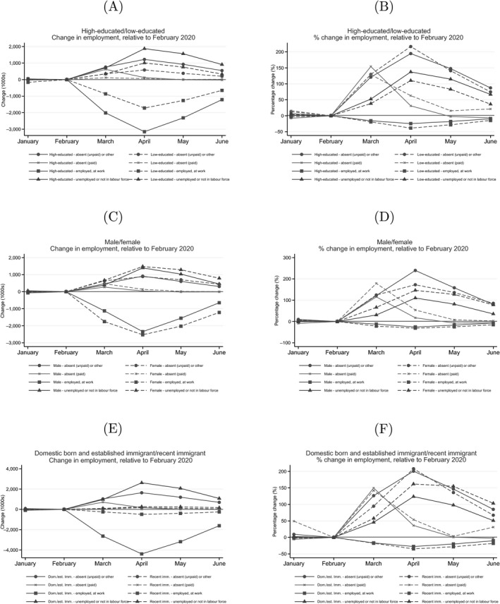
Breakdown of employment loss by demographics

NOTE: Changes in employment are computed relative to February and percent changes are normalized using the February level of employment.

The education breakdowns in the first row of figure 11 reflect our earlier observation that lower‐educated workers faced relatively larger declines in being employed/working and increases in being employed/absent. Although low‐educated workers make up about one quarter of total employment, their employed/working loss was nearly half as large as that of high‐educated workers between February and April or February and June. For both education groups, decreases in employed/working were allocated approximately two thirds/one third to the non‐employed and employed/absent categories, respectively.

The middle row of figure 11 shows that employed/working losses were greater for women than for men. For women, employed/working declines came from greater percentage increases in being non‐employed and lower increases in being employed/absent from work than for men. Finally, recent immigrants faced similar percentage increases in being employed/absent but larger increases in being non‐employed than other workers. That is, they are relatively more likely to be simply thrown out of work without a maintained connection to the firm.

The employed/absent/paid state represents a potential form of income insurance for workers—though one that is little used. It is less clear how to think about the employed/absent/unpaid state. It is worse than being employed/working and similar to being unemployed in terms of income loss. However, it represents a remaining connection to the firm that may confer an advantage by allowing a more rapid return to work.

To understand the nature of the employed/absent categories, we examine the probability of being employed/working in June for individuals who were not employed/working in April. To do this, we take advantage of the “minipanel” nature of the LFS. We examine individuals who are not employed/working in April and break them down into five groups: (i) employed/absent/paid, (ii) employed/absent/unpaid, (iii) unemployed/temporary layoffs, (iv) other unemployed and (v) not in the labour force. For each group, we then calculate the proportion who are employed/working in June.15 ^, 16

The best non‐working state in terms of future access to work is employed/absent/paid, with 61.4% of individuals employed/working in June. This is not surprising given it represents a situation in which the worker is still attached to the firm and the firm may want to have the individual work because it is still paying them. However, we have seen that this is a very small group. In comparison, 49.1% of individuals who are absent/employed/not paid in April are employed/working by June, placing them almost midway between the unemployed/temporary layoffs (58.7%) and the rest of the unemployed (39.7%), who in principle have no formal ongoing connection with their former employer.17 Thus, being employed/absent represents a connection to the firm that does have some value, though less than is reflected in being placed on temporary layoff.

Assessing whether any demographic group has benefited from the expansion of the employed/absent state is not straightforward. From figure 11, we know that more‐educated workers faced smaller declines in the employed/working state. Because this is the preferred labour market state, we can conclude that the combination of labour demand shocks and adjustments through labour hoarding have been relatively favourable to high‐educated workers. However, conditional on not being employed/working, the low‐educated were relatively more likely to move into the employed/absent state rather than the non‐employed state. This represents a relative advantage in reconnecting to work in the future for those not currently working. In the gender breakdown, on the other hand, the patterns all point in the same direction. Men faced smaller declines in employed/working and, for those who were not in this state, larger increases in being employed/absent relative to being non‐employed. Thus, females faced larger increases in the least desirable state and larger declines in the most desirable state. The same holds for recent immigrants: they have had both larger declines in the state of employed/working and larger increases in the state of being non‐employed.

In figure 12, we present ratios of the probabilities of being in the employed/working state for males/females, high‐educated/low‐educated and non‐immigrants/immigrants broken down by the different April labour market states.18 For each origin (non‐working) state, females have a much lower probability of working in June. This relative disadvantage is greater in the employed/absent/not paid state than the unemployed (not on temporary layoff) state. Thus, women have lower access to the employed/absent option and even when they have it are at a greater than normal disadvantage in terms of being called back to work from that state. Recent immigrants, similarly, experience much lower rates of moving back to work in June but for them it is the unemployed who fare relatively worse in this regard. In contrast, there is little difference between the more‐ and lower‐educated in terms of their probability of working in June for all categories other than the (small) employed/absent/paid state.

FIGURE 12.

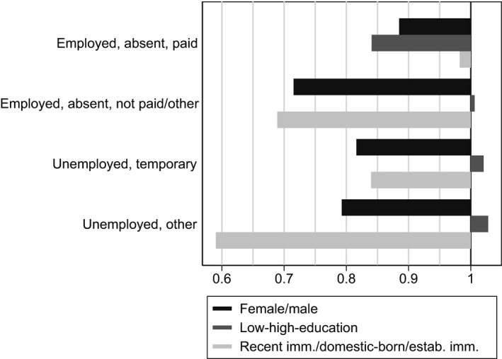
Probability of employment in June by non‐work state in April, group ratios

NOTES: Ratios of proportions of people who were in each of the listed states in April 2020 and who were employed and at work in the LFS survey week in June 2020. Based on longitudinal LFS data.

6.2. Adjustment by working from home

The greater probability of working for males/high‐educated/non‐recent immigrants may arise because of another adjustment mechanism that has risen to relevance in this particular recession: working from home. To establish the importance of this adjustment mechanism and who is able to access it, we estimate regressions using the proportion of workers in a given occupation who reported working from home as a response to the pandemic. In particular, in April, the LFS introduced a question asking workers if they worked from home in the reference week but usually worked outside the home. In April, May and June, only one of the six rotations was asked this question, while in July, five of the six rotations were asked.19 The work‐from‐home variable is restricted to workers who were employed and not absent from work.

We compute the proportion of employed/working individuals who report that they are working at home but don't usually do so. Overall, in April through July 2020, about one fifth (20.8%) of workers are newly working from home but there are substantial differences across groups. Women are more likely to have shifted their work to home (23.9%, compared with 18.3% for men). This may suggest an advantage to women in terms of having access to this adjustment mechanism but likely reflects a greater tendency for women relative to men to work from home in order to take care of children who can no longer go to school. In that sense, it would suggest an added work disadvantage for women to the extent that working from home with children present creates issues for productivity and career progress.

The biggest difference in working from home is between the low‐ and high‐educated groups. One quarter (25.1%) of the high‐educated were newly working from home after the onset of COVID‐19, but only 6.3% of the low‐educated made this change.20 One way to put this difference in context is to do a simple counterfactual exercise in which we ask what the June employment level would have been for the low‐educated if their rate of working from home had increased to the same extent as the high‐educated. In doing this, we assume that the increase in people working from home would be drawn entirely from the set of non‐workers rather than just a conversion from those who are working but not from home in June. In this sense, our counterfactual is an upper bound on what increasing the option of working from home would do to employment for the low‐educated. The counterfactual exercise yields an estimate of an increase by approximately 100,000 in the number of low‐educated employees in June 2020. Going back to figure 4, we see this represents about a quarter of the total job loss for this group between February and June. In percentage terms, it would imply a decline of just over 6% instead of 9%. This is the same percentage decline experienced by the high‐educated. That is, according to our rough counterfactual, we can completely account for the extra job loss for the low‐educated through their lower access to the “work‐from‐home” adjustment mechanism.

6.3. Co‐insurance and household structure

Exposure to both virus and employment risk could be either amplified or mitigated within the household. In particular, if those who work in high‐risk occupations tend to live with others in high‐risk occupations, then the exposure for a given household is magnified. In figure 13, we examine risk sharing in terms of job loss for couples. Given the focus on couples, we take a slightly different approach than in the rest of the paper. We restrict analysis to the January and February 2020 rotation samples because we are able to obtain pre‐COVID‐19 occupation and household earnings information; then, using the longitudinal component of the LFS, we follow these two cohorts from February to June. We examine the employment outcomes in terms of occupational risk and household earnings, which we define on the basis of the February 2020 values. We categorize low‐risk households as those for which neither spouse worked in a high‐risk or health occupation in February and a high‐risk household as those for which at least one person of the couple worked in either a high‐risk or health occupation. We show the fraction of each earning/risk category for which both are employed, the male is employed and the female is not employed, the female is employed and the male is not employed, or both are not employed.

FIGURE 13.

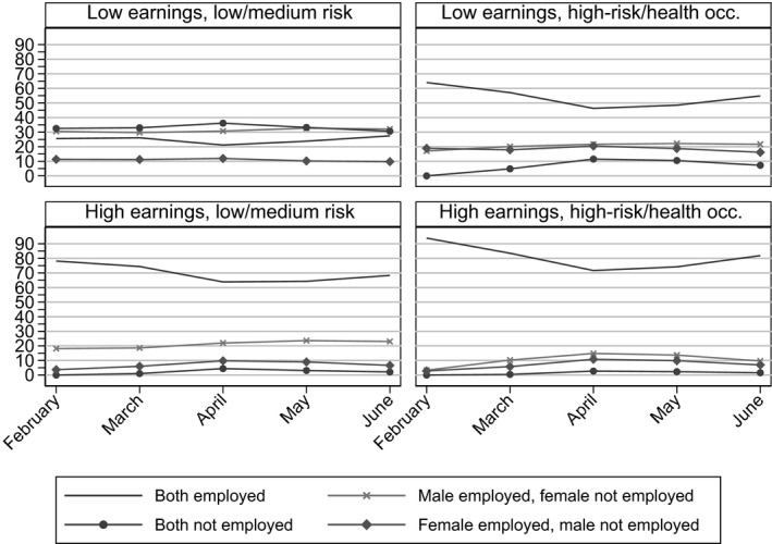
Employment outcomes by household earnings and viral risk

NOTES: Sample restricted to the 2020 January and February rotations. Household earnings and individual risk index/occupation determined in February 2020.

Our analysis of job loss in section 4 revealed that workers in occupations with higher VSE Risk Index scores experienced greater job loss. Here, we find the same viral risk‐job loss relationship on the basis of the household analysis. While there is a sizeable decline between February and April in terms of households in which both spouses are employed for all four risk–earnings groups, we find that household with at least one worker in an occupation with a high VSE Risk Index score see a disproportionate decline. This is true even though we have included health occupations in this group and healthcare job loss was minimal. The fraction of high‐earnings/high‐risk households in which both members of the couple were employed declined from 94% in February to 72% in April, while the fraction for the low‐earnings/high‐risk households declined from 64% to 46% over the same period. The low‐risk groups also experienced declines in the proportion of couples in which both were employed, but to a lesser degree.

We can get an assessment of within‐family employment insurance by examining movements in the proportion of couples in which both were not employed. For low‐earning households of both risk levels, the decline in the proportion with both employed is almost exactly mirrored by the proportion in which neither worked. In contrast, in the high‐earnings households, the movement in the proportion of couples in which both are not working is minimal. That is, high‐earnings couples were able to continue with at least one member of the couple in work while low‐earnings couples were not. Thus, to the extent that low earnings are correlated with low education, the larger job losses for lower‐educated workers is amplified by their household matches. Lower‐educated (low‐earning) workers are more likely to have a spouse who also loses a job. Thus, they not only face greater job risk but also have lower intrahousehold insurance against that risk.

7. Conclusion

The COVID‐19 pandemic has revealed the important inequalities between workers in terms of their exposure to disease and to job loss, as well as the relationship that exists between the two forms of risk. In this paper, we characterize the distribution of both risks, and how they interact differently for women, low‐educated workers and recent immigrants.

At the onset of the pandemic, we worked closely with public health authorities in British Columbia and Quebec to develop a risk index that could be used to plan the economic response to the crisis, the VSE Risk Index. The creation of this index constitutes our first contribution. While others before us have recognized the importance of job characteristics, input from public health officials and access to highly disaggregated data allowed us to incorporate worker characteristics into the measure and evaluation of risk. In this paper, we show that, for certain groups—like immigrants—characterizing risk only in terms of risk related to at‐work characteristics misses out on an important dimension of viral risk. Furthermore, we find evidence that at‐work risk components typically used until now may in part proxy for risk faced by workers through their living arrangements. This is an important policy consideration going forward, as much of the debate on viral containment has focused on the work place.

Our second contribution is to characterize how viral and employment risk, as well as the relationship between the two, vary across various subgroups. We find that the VSE Risk Index is strongly correlated with the proportion of women in an occupation, but bears no systematic relationship with other occupation‐level worker characteristics, such as the prevalence of low‐education workers. Women experienced large employment losses through the pandemic, contrasting with typical male‐dominated employment losses in recent recessions. In comparison, low‐educated workers and immigrants were hit most substantially by the “pandemic” recession, even though we find no evidence that occupations with higher proportions of either group were at greater risk of viral contagion.

While health occupations were among the riskiest in terms of viral contagion, the nature of the crisis was such that they experienced the smallest employment losses. Among non‐health occupations, however, we find a strong and positive relationship between viral risk and employment losses. At the peak of confinement, in April, high‐risk occupations had lost 26.5% of employment, compared with less than 10% in low‐risk occupations. Furthermore, while low‐risk occupations had fully recovered by June, high‐risk occupations were still 15.5% below the February employment levels. In great part, the net effect of the pandemic on employment, with respect to risk, can be explained by the fact that high‐risk occupations were more likely to lose employment but no more likely to regain employment after April. We show that the correlation between viral risk and employment loss was driven by occupations in which workers perform job tasks in close physical proximity to others. However, this factor appears to proxy at least in part for economic disadvantage. Indeed, in regressions of occupation‐level employment loss on at‐work and at‐home risk components, we find that controlling for the share of workers who live in crowded dwellings substantially reduces the size of the coefficient on proximity.

Thus, both types of risk that we examine—risk of exposure to the virus and risk of job loss—increased in ways that reflect deep‐seated inequalities in Canadian society. Women have faced greater virus risk exposure because of the occupations in which they tend to work. That greater risk exposure combined with the fact that high‐risk occupations were more likely to lose employment completely explains the higher job loss for women, especially when measured relative to earlier recessions. Moreover, they had lower probabilities than men of being employed but absent from work, i.e., to maintaining a connection to the firm that turned out to improve workers’ abilities to reconnect with employment during the recovery phase. They were also more likely than men to shift to working from home, which is likely reflects their making sacrifices related to work in order to care for children at home. At the same time, women did not face higher rates of layoff within occupations of a given risk type. That is, women were not more likely to be laid off simply because they were women.

In contrast, low‐educated workers did not face higher exposure to virus risk on the job but were much more likely to be laid off than high‐educated workers. This fits with observations in previous recessions that the low‐educated bear the brunt of job loss. We present a rough counterfactual exercise that implies that in the COVID‐19 recession, the extra job loss for the low‐educated can be accounted for by their lower propensity to switch to working from home.

Taken together, our results reveal the ways in which the COVID‐19 crisis exposed the deep inequities in our society. Women faced more virus risk and were given less access to ongoing connections to the firm because of long‐standing occupational patterns and the division of work within the home. Low‐educated workers faced employment losses because their living arrangements made it less possible for them to adjust to the labour demand shock induced as a necessary response to COVID‐19. The virus may affect us all but it moves through existing structures to increase inequality.

Additional figures

To characterize the distribution of risk more completely, we also estimate nine quantile regressions (for quantiles 0.1, 0.2, …, and 0.9), using the same set of variables as in figure 3, panel B, and present the corresponding estimated coefficients in figure A2. The marginal effect of a one standard deviation increase in the proportion of female workers is always positive. Moreover, it is smaller at the bottom of the risk distribution and greater at the top. Hence, risk is distributed more unequally in high female‐proportion occupations than in low female‐proportion occupations, with female dominated occupations being particularly concentrated in high‐risk characteristics. The results for high‐immigrant occupations indicate that their distribution of risk is more right‐skewed than it is for the low‐immigrant occupations, which could relate to a greater tendency to have lower contact with the public.

FIGURE A1.

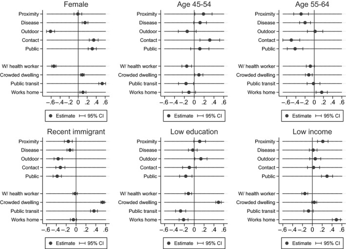
Regression of risk factors on occupation‐level characteristics: Excluding health occupations

NOTES: Point estimates and 95% confidence intervals of risk components regressed on demographic characteristics of four‐digit NOC occupations. Results come from multivariate regressions of each risk component on the set of demographic characteristics. Each panel presents the marginal effect of the corresponding characteristic in each of these regressions.

FIGURE A2.

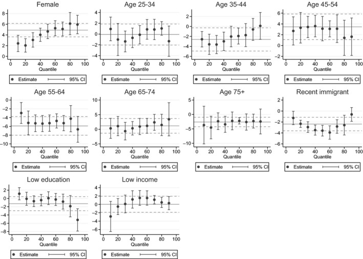
Quantile regression of risk on occupation‐level characteristics: All occupations

NOTES: Point estimates and 95% confidence intervals of VSE Risk Index regressed on demographic characteristics of four‐digit NOC occupations. Solid horizontal lines reproduce estimates presented in figure 3 and dashed lines, the corresponding 95% confidence intervals.

FIGURE A3.

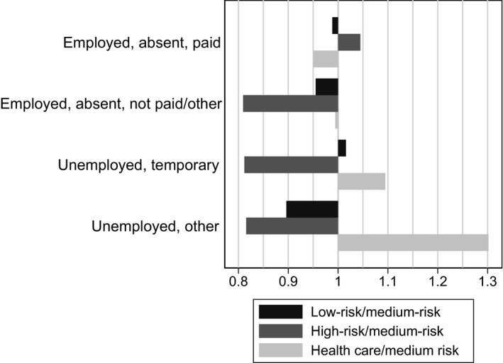
Probability of employment in June by non‐work state in April, group ratios

NOTES: Ratios of proportions of people who were in each of the listed states in April 2020 and who were employed and at work in the LFS survey week in June 2020. Based on longitudinal LFS data.

References

- de Beyer, J. , and Knight J. B. (1989) “The role of occupation in the determination of wages,” Oxford Economic Papers 41(3), 595–618 [Google Scholar]
- Chernoff, A.W. , and Warman C. (2020) “COVID‐19 and implications for automation,” NBER working papers no. 27249
- Cortes, G.M. , and Forsythe E. C. (2020) “The heterogeneous labor market impacts of the COVID‐19 pandemic,” Upjohn Working Papers and Journal Articles, no. 20‐327 [DOI] [PMC free article] [PubMed]
- Delaney, J.M. , and Devereux P. J. (2019) “More education, less volatility? The effect of education on earnings volatility over the life cycle,” Journal of Labor Economics 37(1), 101–37 [Google Scholar]
- Deming, D. , and Kahn L. B. (2018) “Skill requirements across firms and labor markets: Evidence from job postings for professionals,” Journal of Labor Economics 36(S1), S337–S369 [Google Scholar]
- Dingel, J.I. , and Neiman B. (2020) “How many jobs can be done at home?” Journal of Public Economics 189, 104235 [DOI] [PMC free article] [PubMed] [Google Scholar]
- Gamio, L. (2020, March 15) “The workers who face the greatest coronavirus risk,” The New York Times
- Green, D.A. , Karimirad A., Simard‐Duplain G., and Siu H. E. (2020) “COVID and the economic importance of in‐person K–12 schooling,” NBER working paper no. 28200 [DOI] [PMC free article] [PubMed]
- Gross, C.P. , Essien U. R., Pasha S., Gross J. R., Wang S.‐Y., and Nunez‐Smith M. (2020) “Racial and ethnic disparities in population‐level COVID‐19 mortality,” Journal of General Internal Medicine 35, 3097–99 [DOI] [PMC free article] [PubMed] [Google Scholar]
- Hoynes, H. , Miller D. L., and Schaller J. (2012) “Who suffers during recessions?,” Journal of Economic Perspectives 26(3), 27–48 [Google Scholar]
- Jaimovich, N. , and Siu H. E. (2009) “The young, the old, and the restless: Demographics and business cycle volatility,” American Economic Review 99(3), 804–26 [Google Scholar]
- Jaimovich, N. , and Siu H. E. (2020) “Job polarization and jobless recoveries,” Review of Economics and Statistics 102(1), 129–47 [Google Scholar]
- Jones, S.R.G. , Lange F., Riddell W. C., and Warman C. (2020) “Waiting for recovery: The Canadian labour market in June 2020,” Canadian Public Policy 46(S2), S102–S118 [DOI] [PMC free article] [PubMed] [Google Scholar]
- Jones, S.R.G. , and Riddell W. C. (2006) “Unemployment and nonemployment: Heterogeneities in labor market states,” Review of Economics and Statistics 88(2), 314–23 [Google Scholar]
- Lemieux, T. , Milligan K., Schirle T., and Skuterud M. (2020) “Initial impacts of the COVID‐19 pandemic on the Canadian labour market,” Canadian Public Policy 46(S1), S55–S65 [DOI] [PMC free article] [PubMed] [Google Scholar]
- Millett, G.A. , Jones A. T., Benkeser D., Baral S., Mercer L., Beyrer C., Honermann B., Lankiewicz E., Mena L., Crowley J. S., Sherwood J., and Sullivan P. S. (2020) “Assessing differential impacts of COVID‐19 on Black communities,” Annals of Epidemiology 47, 37–44 [DOI] [PMC free article] [PubMed] [Google Scholar]
- Mongey, S. , and Weinberg A. (2020) “Characteristics of workers in low work‐from‐home and high personal‐proximity occupations,” BFI white paper
- Mongey, S. , Pilossoph L., and Weinberg A. (2020) “Which workers bear the burden of social distancing policies?,” BFI working paper no. 2020‐51 [DOI] [PMC free article] [PubMed]
- Montenovo, L. , Jiang X., Rojas F. L., Schmutte I. M., Simon K. I., Weinberg B. A., and Wing C. (2020) “Determinants of disparities in COVID‐19 job losses,” NBER working paper no. 27132 [DOI] [PMC free article] [PubMed]
- Price‐Haywood, E.G. , Burton J., Fort D., and Seoane L. (2020) “Hospitalization and mortality among Black patients and White patients with COVID‐19,” New England Journal of Medicine 382(26), 2534–43 [DOI] [PMC free article] [PubMed] [Google Scholar]
- Vu, V. , and Malli N. (2020) “Anything but static: Risks of COVID‐19 to workers in Canada,” www.brookfieldinstitute.ca/p/7991