Extinction and stationary distribution of a stochastic COVID-19 epidemic model with time-delay

Abstract

We reformulate a stochastic epidemic model consisting of four human classes. We show that there exists a unique positive solution to the proposed model. The stochastic basic reproduction number $R_0^s$ is established. A stationary distribution (SD) under several conditions is obtained by incorporating stochastic Lyapunov function. The extinction for the proposed disease model is obtained by using the local martingale theorem. The first order stochastic Runge-Kutta method is taken into account to depict the numerical simulations.

1. Introduction

The outspread of infectious diseases like COVID-19 have been reported employing mathematical models such as stochastic and deterministic. Almost all models are the offshoots of a classical SIR model by Kermack Mckendrick [1]. SIR model is sub-divided in three groups such as susceptible S, infected I and recovered R population. The primary framework of the disease in a population is associated with the rate of incidence. It is therefore related with the mean of secondary cases evolved by an infected individual in the susceptible population. Many descendent models have been employed after Kermack McKendrick model [2,3]. The variations in our social and environmental differences in our daily life are the justifications of establishing stochastic integration in such models. Stochastic noise of a model reshapes the solution behavior of correlated deterministic system and also changes the threshold level of a system for an epidemic to occur. The noise induction affects the dynamics of the population [4]. An epidemiological infection with a source of noise with memory was employed with a dynamical model [5]. The epidemic dynamics model was analyzed by employing pulse noise model. Elsewhere threshold variation is described to examine the stochastic SIR model [6]. An increasing attention has been noticed for the analysis and control of COVID-19, also for vaccination and treatment policies. The association of vaccination or other treatment strategies and their relation with the transmission of a disease has been a hot topic for theoretical and applied analysis [[7], [8], [9], [10], [11], [12], [13], [14], [15], [16], [17], [18], [19], [20], [21]]. The disease transmission modeling in a population where vaccination is under effect, the main issue is the inefficiency of the vaccine in a given population. There is a possibility of low efficacy such as partial induction of immunization. Considering SIR-type disease such as COVID-19 during the vaccination program is in effect, the total population is divided into four classes i.e susceptible, infected, vaccinated and removed represented as S, I, V, and R respectively. (see Table 1 )

$$\begin{array}{cc}\frac{dS}{dt}& =\mu -\beta SI(t-\tau )-(\mu +\phi )S(t)+\theta V(t),\\ \frac{dI}{dt}& =\beta S(t)I(t-\tau )+\rho \beta V(t)I(t)-(\lambda +\mu )I(t),\\ \frac{dV}{dt}& =\phi S(t)-\rho \beta V(t)I(t)-(\mu +\theta )V(t),\\ \frac{dR}{dt}& =\lambda I(t)-\mu R(t).\end{array}$$ (1)

Table 1.

List of parameters.

	Test 1	Test 2	Test 3	Test 4	Test 5	Test 6
Β	0.038 9	0.043 0	0.953 7	0.953 7	0.509 0	0.255 9
Φ	0.918 5	0.823 9	0.004 8	0.004 8	0.484 9	0.280 3
Θ	0.866 3	0.882 4	0.944 4	0.944 4	0.731 9	0.363 8
Δ	0.032 7	0.666 7	0.128 1	0.128 1	0.285 1	0.666 2
Ρ	0.947 3	0.255 3	0.349 4	0.349 4	0.437 8	0.149 5
σ1	0.080 1	0.037 4	0.131 8	0.131 8	0.192 1	0.096 1
σ2	0.349 2	0.669 8	0.276 4	0.276 4	0.107 8	0.570 0
σ3	0.038 8	0.235 1	0.220 6	0.220 6	0.159 8	0.095 3
σ4	0.081 2	0.054 5	0.047 6	0.047 6	0.041 3	0.132 1
S0	0.240 9	0.801 9	0.740 6	0.740 6	0.456 7	0.434 3
V0	0.635 3	0.498 1	0.280 3	0.280 3	0.081 0	0.725 6
R0	0.831 1	0.814 3	0.818 1	0.818 1	0.441 5	0.276 6
Τ	50Δt	100Δt	200Δt	300Δt	500Δt	1000Δt

The basic reproduction number of this model is $R_0=\frac{\beta }{\mu +\lambda }$. In this model, it is assumed that during a given time, a fraction of the susceptible class is vaccinated. The vaccination may or may not immunize the individual, so the model includes ρ factor which is 0 < ρ < 1, where ρ = 0 refers to the effectiveness of the vaccine and ρ = 1 refers to the non-effectiveness of the vaccine. We also assume that the effect of vaccine is lost at some rate of proportion θ. Therefore, since the immunity is long lasting hence a fraction λ of infective goes to the removed class. It is also supposed that birth rate of the population takes place at a constant rate m of death and the neonates move into susceptible class. Thus, the overall population is constant and variables are normalized. In this study, we observed as a case where the vaccine is effective (θ = 0). This model can be further modified according to the environment of the system. The stochastic version of the above model is presented as:

$$\begin{array}{cc}dS& =[\mu -\beta SI(t-\tau )-(\mu +\phi )S(t)+\theta V(t)]dt+{\sigma }_{1}Sd{W}_1(t),\\ dI& =[\beta S(t)I(t-\tau )+\rho \beta V(t)I(t)-(\lambda +\mu )I(t)]dt+{\sigma }_{2}Id{W}_2(t),\\ dV& =[\phi S(t)-\rho \beta V(t)I(t)-(\mu +\theta )V(t)]dt+{\sigma }_{3}Vd{W}_3(t),\\ dR& =[\lambda I(t)-\mu R(t)]dt+{\sigma }_{4}Rd{W}_4(t),\end{array}$$ (2)

where W ₁(t), W ₂(t), W ₃(t) and W ₄(t) stand for the independent Brownian motions. ${\sigma }_1^2$, ${\sigma }_2^2,{\sigma }_3^2$ and ${\sigma }_4^2$ are white noises, with ICs:

$$\begin{array}{cc}S(\phi )& ={\zeta }_1(\phi ),I(\phi )={\zeta }_2(\phi ),\\ V(\phi )& ={\zeta }_3(\phi ),R(\phi )={\zeta }_4(\phi ),\phi \in [-\tau ,0],\\ & {\phi }_i(\phi )\in C,i=1,2,3,4.\end{array}$$ (3)

This paper is presented as follows: The existence and uniqueness have been carried out in Section 2. In Section 3, Extinction analysis of the underlying model is investigated. In Section 4, the existence of ergodic stationary distribution. Numerical simulations by using first order stochastic Runge-Kutta scheme is demonstrated in Section 5. In the last section i.e 6, concluding remarks are presented.

2. Existence and uniqueness

As the solution of SDE (2) has biological significance, it should be nonnegative [22]. Moreover, in order for a stochastic differential equation to have a unique global (i.e., no explosion in a finite time) solution for any given initial value, the coefficients of the equation are generally required to satisfy a linear growth condition and a local Lipschitz condition [23]. However, the coefficients of SDE (2) do not satisfy a linear growth condition, though they are locally Lipschitz continuous. In this section, we will use a method similar to the proof of [24,25], to prove that the solution of SDE (2) is nonnegative and global.

Theorem 1

System (2) has a unique positive solution (S(t), I(t), V(t), R(t)) on t ≥ − τ, and the solution will remain in ${\mathbb{R}}_{+}^4$ for the given initial condition (3) with probability one.

Proof 1

We define a C ² − function $V:{\mathbb{R}}_{+}^4\to {\mathbb{R}}_{+}$ as follows:

$$\mathcal{V}(S,I,V,R)=\left(S-k-k\frac{\ln S}{k}\right)+(I-1-\ln I)+(V-1-\ln V)+(R-1-\ln R)+{\int }_t^{t+\tau }k\beta I(s-\tau )ds,$$

where k > 0 will be determined later on. By Ito's formula, we can obtain

$$d\mathcal{V}=\mathcal{LV}dt+{\sigma }_1(S-k)d{W}_1(t)+{\sigma }_2(I-1)d{W}_2(t)+{\sigma }_3(V-1)d{W}_3(t)+{\sigma }_4(R-1)d{W}_4(t),$$

where

$$\begin{array}{cc}\mathcal{LV}& =\left(1-\frac{k}{S}\right)(\mu -\beta SI(t-\tau )-(\mu +\phi )S(t)+\theta V(t))+\left(1-\frac{1}{I}\right)(\beta S(t)I(t-\tau )+\rho \beta V(t)I(t)-(\lambda +\mu )I(t))\\ & +\left(1-\frac{1}{V}\right)(\phi S(t)-\rho \beta V(t)I(t)-(\mu +\theta )V(t))+\left(1-\frac{1}{R}\right)(\lambda I(t)-\mu R(t))\\ & +\frac{k{\sigma }_1^2+{\sigma }_2^2+{\sigma }_3^2+{\sigma }_4^2}{2}+k\beta I(t)-k\beta I(t-\tau )\end{array}$$

$$\le 4\mu +\phi +\lambda +\theta -\mu S-\rho \beta V+[\beta (\rho +k)-\mu ]-\mu V+\frac{k{\sigma }_1^2+{\sigma }_2^2+{\sigma }_3^2+{\sigma }_4^2}{2}.$$

Let $k=\frac{\mu -\rho \beta }{\beta }$, then we have

$$\mathcal{LV}\le 4\mu +\phi +\lambda +\theta +\frac{k{\sigma }_1^2+{\sigma }_2^2+{\sigma }_3^2+{\sigma }_4^2}{2}\le \mathcal{M},$$ (4)

where $\mathcal{M}>0$. Hence,

$$d\mathcal{V}(S,I,V,R)=\mathcal{M}dt+{\sigma }_1(S-k)d{W}_1(t)+{\sigma }_2(I-1)d{W}_2(t)+{\sigma }_3(V-1)d{W}_3(t)+{\sigma }_4(R-1)d{W}_4(t).$$ (5)

Integrating (6) from 0 to ${\tau }_n\wedge \tilde{T}=\min \{{\tau }_n,\tilde{T}\}$ leads us

$$\mathcal{WV}\left(S({\tau }_n\wedge \tilde{T}),I({\tau }_n\wedge \tilde{T}),V({\tau }_n\wedge \tilde{T}),R({\tau }_n\wedge \tilde{T})\right)\le \mathcal{WV}\left(S(0),I(0),V(0),R(0)\right)+\mathcal{M}\tilde{T}.$$ (6)

implies

$$\mathcal{V}\left(S({\tau }_n\wedge \tilde{T}),I({\tau }_n\wedge \tilde{T}),V({\tau }_n\wedge \tilde{T}),R({\tau }_n\wedge \tilde{T})\right)\ge (n-1-\ln n)\wedge \left(\frac{1}{n}-1-\ln \frac{1}{n}\right).$$ (7)

According to (7), we get

$$\begin{array}{r}\hfill \mathcal{GV}(S(0),I(0),V(0),R(0))+\mathcal{M}\tilde{T}\ge \mathcal{G}[1_{{\mathrm{\Omega }}_n(\omega )}\mathcal{V}\left(S({\tau }_n,\omega ),I({\tau }_n,\omega ),V({\tau }_n,\omega ),R({\tau }_n,\omega )\right)]\\ \hfill \ge \epsilon (n-1-\ln n)\wedge \left(\frac{1}{n}-1-\ln \frac{1}{n}\right),\end{array}$$ (8)

limiting case leads us

$$\infty >\mathcal{GV}(S(0),I(0),V(0),R(0))+\mathcal{M}\tilde{T}=\infty ,$$ (9)

contradiction arises hence τ _∞ = ∞, a.s.

3. Extinction

In this section, we will show that if the noise is sufficiently large, the solution to the associated SDE (2) will become extinct with probability 1 [[26], [27], [28]].

Lemma 1

Let$M={\{M_t\}}_{t\ge 0}$be a real-valued continuous local martingale vanishing at t = 0, and${⟨M,M⟩}_t$be the quadratic variation of M. Then

$\underset{t\to \infty }{\lim }{⟨M,M⟩}_t=\infty ,a.s.\Rightarrow \underset{t\to \infty }{\lim }\frac{M_t}{{⟨M,M⟩}_t}=0a.s$.,

and also.

$\underset{t\to \infty }{\lim }\sup \frac{{⟨M,M⟩}_t}{t}<\infty a.s.\Rightarrow \underset{t\to \infty }{\lim }\frac{M_t}{t}=0,a.s.$,

Lemma 2

Let (S(t), I(t), V(t), R(t)) be the solution of (2) with any $(S(0),I(0),V(0),R(0))\in {\mathbb{R}}_{+}^4$, then

$\underset{t\to \infty }{\lim }\frac{S(t)}{t}=0,\underset{t\to \infty }{\lim }\frac{I(t)}{t}=0,\underset{t\to \infty }{\lim }\frac{V(t)}{t}=0,\underset{\to \infty }{\lim }\frac{R(t)}{t}=0,a.s$.,

Furthermore, if$\mu >\frac{{\sigma }_1^2\vee {\sigma }_2^2\vee {\sigma }_3^2\vee {\sigma }_4^2}{2}$, then.

$\underset{t\to \infty }{\lim }\frac{{\int }_0^{t}S(s)d{W}_1(s)}{t}=0,\underset{t\to \infty }{\lim }\frac{{\int }_0^{t}I(s)d{W}_2(s)}{t}=0,\underset{t\to \infty }{\lim }\frac{{\int }_0^{t}V(s)d{W}_3(s)}{t}=0$,

$\underset{t\to \infty }{\lim }\frac{{\int }_0^{t}R(s)d{W}_4(s)}{t}=0$, a.s.

Theorem 2

If$R_0^s<1$and$\mu >\frac{{\sigma }_1^2\vee {\sigma }_2^2\vee {\sigma }_3^2\vee {\sigma }_4^2}{2},$then (2) obeys:

$$\begin{array}{c}\lim S_{t\to \infty }\sup \frac{1}{t}\ln (\lambda (I+V)+(\lambda +\mu )R)\le (\beta +\lambda \phi )Sdt-\frac{1}{2{(\lambda )}^2}\left\{{\lambda }^2\right)\frac{{\sigma }_2^2}{2}\wedge \left({\lambda }^2\left(\mu +\theta +\frac{{\sigma }_3^2}{2}\right)\right)\\ \left(\wedge \left(\lambda +\mu (1-\lambda -\mu )+\frac{{\sigma }_3^2}{2}\right)\right\}<0and\underset{t\to \infty }{\lim }⟨S⟩=1,a.s.\end{array}$$

Proof 2

Let $\mathcal{U}(t)=\lambda (I+V)+(\lambda +\mu )R$, and applying Ito's formula leads us,

$$\begin{array}{cc}d\ln \mathcal{U}(t)& =\left\{\frac{1}{\lambda (I+V)+(\lambda +\mu )R}[\lambda \beta SI(t-\tau )+\lambda \phi S-\lambda (\mu +\theta )V-\mu (\lambda +\mu )R\mu ]\right)\\ & \left(-\frac{{\lambda }^2{\sigma }_2^2{I}^2+{\lambda }^2{\sigma }_3^2{V}^2+{(\lambda +\mu )}^2{\sigma }_4^2{R}^2}{2{(\lambda (I+V)+(\lambda +\mu )R)}^2}\right\}dt+\frac{{\lambda }_2{\sigma }_{2}I}{\lambda (I+V)+(\lambda +\mu )R}d{W}_2\end{array}$$

$$+\frac{{\lambda }_2{\sigma }_{3}V}{\lambda (I+V)+(\lambda +\mu )R}d{W}_3+\frac{{\sigma }_4(\lambda +\mu )R}{\lambda (I+V)+(\lambda +\mu )R}d{W}_4$$

$$\begin{array}{cc}\le & (\beta +\lambda \phi )Sdt-\frac{1}{\lambda (I+V)+(\lambda +\mu )R}\left\{{\lambda }^2\frac{{\sigma }_2^2}{2}{I}^2+{\lambda }^2\left(\mu +\theta +\frac{{\sigma }_3^2}{2}\right)V^2\right)\\ & \left(+\left(\lambda +\mu (1-\lambda -\mu )+\frac{{\sigma }_4^2}{2}\right)R^2\right\}dt+\frac{{\lambda }_2{\sigma }_{2}I}{\lambda (I+V)+(\lambda +\mu )R}d{W}_2\\ & +\frac{{\lambda }_2{\sigma }_{3}V}{\lambda (I+V)+(\lambda +\mu )R}d{W}_3+\frac{{\sigma }_4(\lambda +\mu )R}{\lambda (I+V)+(\lambda +\mu )R}d{W}_4\end{array}$$

$$\le (\beta +\lambda \phi )Sdt-\frac{1}{2{(\lambda )}^2}\left\{{\lambda }^2\frac{{\sigma }_2^2}{2}\wedge \left({\lambda }^2\right)\left(\mu +\theta +\frac{{\sigma }_3^2}{2}\right)\wedge \left(\lambda +\mu (1-\lambda -\mu )+\frac{{\sigma }_3^2}{2}\right)\right\}dt$$

$$+\frac{{\lambda }_2{\sigma }_{2}I}{\lambda (I+V)+(\lambda +\mu )R}d{W}_2+\frac{{\lambda }_2{\sigma }_{3}V}{\lambda (I+V)+(\lambda +\mu )R}d{W}_3$$

$$+\frac{{\sigma }_4(\lambda +\mu )R}{\lambda (I+V)+(\lambda +\mu )R}d{W}_4.$$ (10)

From model (2), we have

$$\begin{array}{c}\hfill d(S+I+V+R)=[\mu -\mu (S+I+V+R)]dt\\ \hfill +{\sigma }_{1}Sd{W}_1+{\sigma }_{2}Id{W}_2+{\sigma }_{3}Vd{W}_3+{\sigma }_{4}Rd{W}_4.\end{array}$$ (11)

Integration gives us

$$⟨S+I+V+R⟩=1+{\psi }_1(t),$$ (12)

where

$$\begin{array}{cc}{\psi }_1& =\frac{1}{\mu }\left[\frac{1}{t}(S(0)+I(0)+V(0)+R(0))\right)-\frac{1}{t}(S(t)+I(t)+V(t)+R(t))+\frac{{\sigma }_1{\int }_0^{t}S(s)d{W}_1}{t}+\frac{{\sigma }_2{\int }_0^{t}I(s)d{W}_2}{t}\\ & +\left(\frac{{\sigma }_3{\int }_0^{t}V(s)d{W}_3}{t}+\frac{{\sigma }_4{\int }_0^{t}R(s)d{W}_4}{t}\right].\end{array}$$ (13)

Using Lemmas 1 and 2,

$$\underset{t\to \infty }{\lim }{\psi }_1(t)=0a.s.$$

limit of (13) gives us,

$$\underset{t\to \infty }{\lim }\sup ⟨S+I+V+R⟩=1,a.s.$$ (14)

Integrating leads us

$$\frac{\ln \mathcal{U}(t)}{t}\le (\beta +\lambda \phi )Sdt-\frac{1}{2{(\lambda )}^2}\left\{{\lambda }^2\frac{{\sigma }_2^2}{2}\wedge \left({\lambda }^2\right)\left(\mu +\theta +\frac{{\sigma }_3^2}{2}\right)\wedge \left(\lambda +\mu (1-\lambda -\mu )+\frac{{\sigma }_3^2}{2}\right)\right\}dt+{\psi }_2,$$ (15)

where

$$\begin{array}{cc}{\psi }_2(t)& =\frac{\ln \mathcal{U}(0)}{t}+\frac{\lambda {\sigma }_2}{t}{\int }_0^t\left(\frac{I(s)}{\lambda (I+V)+(\lambda +\mu )R}d{W}_2\right)\\ & +\frac{\lambda {\sigma }_3}{t}{\int }_0^t\left(\frac{V(s)}{\lambda (I+V)+(\lambda +\mu )R}d{W}_3\right)\\ & +\frac{(\lambda +\mu ){\sigma }_4}{t}{\int }_0^t\left(\frac{R(s)}{\lambda (I+V)+(\lambda +\mu )R}d{W}_4\right).\end{array}$$

Incorporating Lemmas 1 and 2.

$\underset{t\to \infty }{\lim }{\psi }_2(t)=0,$a.s.

Since $R_0^s<1$, limit of (15) leads us

$$\begin{array}{c}\underset{t\to \infty }{\lim }\sup \frac{\ln \mathcal{U}(t)}{t}\hfill \\ \le (\beta +\lambda \phi )Sdt-\frac{1}{2{(\lambda )}^2}\left\{{\lambda }^2\frac{{\sigma }_2^2}{2}\wedge \left({\lambda }^2\right)\left(\mu +\theta +\frac{{\sigma }_3^2}{2}\right)\wedge \left(\lambda +\mu (1-\lambda -\mu )+\frac{{\sigma }_3^2}{2}\right)\right\}dt<0,\hfill \end{array}$$ (16)

implying $\underset{t\to \infty }{\lim }I(t)=0,\underset{t\to \infty }{\lim }V(t)=0,\underset{t\to \infty }{\lim }R(t)=0$ a.s.

From (14), we have $\underset{t\to \infty }{\lim }⟨S⟩=1,a.s$.

4. Stationary distribution

Herein, we construct a suitable stochastic Lyapunov function to study the existence of a unique ergodic stationary distribution [29,30] of the positive solutions to the system (2).

Consider

$$R_0^s=\frac{\phi \rho \beta \mu }{\widehat{\lambda }\widehat{\theta }\widehat{\phi }\widehat{\mu }},$$ (17)

where $\widehat{\lambda }=\frac{\phi \rho \beta \mu }{(\lambda +\mu +\frac{{\sigma }_2^2}{2})},\widehat{\theta }=\frac{\phi \rho \beta \mu }{(\mu +\theta +\frac{{\sigma }_3^2}{2})},\widehat{\phi }=\mu +\phi +\frac{{\sigma }_1^2}{2}$ and $\widehat{\mu }=\mu +\frac{{\sigma }_4^2}{2}$.

Theorem 3

Assume that$R_0^s>1$and$\mu -\frac{{\sigma }_1^2\vee {\sigma }_2^2\vee {\sigma }_3^2\vee {\sigma }_4^2}{2}>0$, then for value$(S(0),E(0),I(0),Q(0))\in {\mathbb{R}}_{+}^4$, then (2) possess SD π(.).

Proof 3

To prove the theorem we take the help of two conditions in Lemma 1 of [24]. For this, we consider the diffusion matrix of model (2) as:

$\mathrm{\Lambda }=\left(\begin{array}{cccc}{v}_1^2{S}^2& 0& 0& 0\\ 0& v_2^2{I}^2& 0& 0\\ 0& 0& v_3^2{V}^2& 0\\ 0& 0& 0& v_4^2{R}^2\end{array}\right)$.

It is easy to show that Λ is positive definite, hence the first condition of Lemma 1 in Ref. [24] is satisfied.

Furthermore, consider ${\mathcal{C}}^2$-function $\mathcal{V}:{\mathbb{R}}_{+}^4\to \mathbb{R}$:

$$\begin{array}{cc}V(S,I,V,R)& =Q\left(-\ln S-c_1\ln I-c_2\ln V-c_3\ln R+\beta {\int }_t^{t+\tau }I(s-\tau )ds\right)\\ & -\ln S+\beta {\int }_t^{t+\tau }I(s-\tau )ds-\ln V-\ln R+\frac{1}{\rho +1}{(S+I+V+R)}^{\xi +1}\\ & =N{V}_1+V_2+V_3+V_4+V_5,\end{array}$$

where $c_1=\frac{\phi \rho \beta \mu }{\lambda +\mu +\frac{{\sigma }_1^2}{2}},c_2=\frac{\phi \rho \beta \mu }{\mu +\theta +\frac{{\sigma }_3^2}{2}}and{c}_3=\frac{\phi \rho \beta \mu }{\mu +\frac{{\sigma }_4^2}{2}}$. Let

$$\begin{array}{ll}\tilde{\mathcal{V}}(S,I,V,R)\hfill & \hfill =\mathcal{Q}\left(-\ln S-c_1\ln I-c_2\ln V-c_3\ln R+\beta {\int }_t^{t+\tau }I(s-\tau )ds\right)-\ln S\\ & \hfill +\beta {\int }_t^{t+\tau }I(s-\tau )ds-\ln V-\ln R+\frac{1}{\rho +1}{(S+I+V+R)}^{\rho +1}\\ & \hfill -V(S(0),I(0),V(0),R(0))\\ & \hfill ≔{\mathcal{NV}}_1+{\mathcal{V}}_2+{\mathcal{V}}_3+{\mathcal{V}}_4+{\mathcal{V}}_5-\mathcal{V}(S(0),I(0),V(0),R(0)),\end{array}$$ (18)

where $(S,I,V,R)\in (\frac{1}{n},n)\times (\frac{1}{n},n)\times (\frac{1}{n},n)\times (\frac{1}{n},n)$ and n > 1.

${\mathcal{V}}_1=-\ln S-c_1\ln I-c_2\ln V-c_3\ln R+\beta {\int }_t^{t+\tau }I(s-\tau )ds$,

${\mathcal{V}}_2=-\ln S+\beta {\int }_t^{t+\tau }I(s-\tau )ds$,

${\mathcal{V}}_3=-\ln V,{\mathcal{V}}_4=-\ln R$,

${\mathcal{V}}_5=\frac{1}{\xi +1}{(S+I+V+R)}^{\xi +1}$,

ξ > 1 is a constant satisfying

$$\mu -\frac{\xi }{2}({\sigma }_1^2\vee {\sigma }_2^2\vee {\sigma }_3^2\vee {\sigma }_4^2)>0,$$

and $\mathcal{N}>0$, obeying

$$-\mathcal{Q}\eta +\mathcal{R}\le -2,$$ (19)

Where $\eta =\frac{\phi \rho \beta \mu }{\widehat{\lambda }\widehat{\theta }}-(\mu +\phi +\frac{{\sigma }_1^2}{2})-c_3(\mu +\frac{{\sigma }_4^2}{2})>0$,

$$\begin{array}{c}\mathcal{R}=\underset{(S,I,V,R)\in {\mathbb{R}}_{+}^4}{\sup }\left(-\frac{1}{4}\left[\mu -\frac{\xi }{2}({\sigma }_1^2\vee {\sigma }_2^2\vee {\sigma }_3^2\vee {\sigma }_4^2)\right]I^{\xi +1}\right)\\ \left(3\mu +\theta +\phi +\beta (1+\rho )I+\mathcal{A}+\frac{{\sigma }_1^2}{2}+\frac{{\sigma }_2^2}{2}+\frac{{\sigma }_3^2}{2}\right),\end{array}$$ (20)

and

$$\begin{array}{c}\mathcal{A}=\underset{(S,I,V,R)\in {\mathbb{R}}_{+}^4}{\sup }\left\{\mu {(S+I+V+R)}^{\rho }-\frac{1}{2}\left[\mu -\frac{\xi }{2}({\sigma }_1^2\vee {\sigma }_2^2\vee {\sigma }_3^2\vee {\sigma }_4^2)\right]\right)\\ \left(\times {(S+I+V+R)}^{\xi +1}\right\}<\infty .\end{array}$$ (21)

Applying Itô’s formula to ${\mathcal{V}}_1$, we have

$$\begin{array}{cc}{\mathcal{LV}}_1& =-\frac{\mu }{S}+\beta I+(\mu +\phi )-\frac{\theta V}{S}-\frac{c_1\beta SI(t-\tau )}{I}-c_1\rho \beta I+c_1(\lambda +\mu )+c_1\frac{{\sigma }_2^2}{2}\\ & -\frac{c_2\phi S}{V}-c_2\rho \beta I+c_2(\mu +\theta )+c_2\frac{{\sigma }_3^2}{2}-\frac{c_3\lambda I}{R}+c_3\mu +c_3\frac{{\sigma }_4^2}{2}\end{array}$$

$$\begin{array}{cc}\le & -3\sqrt[3]{\phi \rho \beta \mu c_1{c}_2}+\mu +\phi +\frac{{\sigma }_1^2}{2}+c_1\left(\lambda +\mu +\frac{{\sigma }_2^2}{2}\right)+c_2\left(\mu +\theta +\frac{{\sigma }_3^2}{2}\right)\\ & c_3\left(\mu +\frac{{\sigma }_4^2}{2}\right)+\beta I(t)+c_2\rho \beta I\end{array}$$

$$\begin{array}{cc}\le & \frac{\phi \rho \beta \mu }{\widehat{\mu }\widehat{\lambda }\widehat{\theta }}+\mu +\phi +\frac{{\sigma }_1^2}{2}+c_3\left(\mu +\frac{{\sigma }_4^2}{2}\right)+\beta I(t)+\beta (1+c_2\rho )I\\ & =-\psi +\beta (1+c_2\rho )I.\end{array}$$ (22)

Similarly, we can get

$${\mathcal{LV}}_2=-\frac{\mu }{S}+(\mu +\phi )-\frac{\theta V}{S}+\beta I+\frac{{\sigma }_1^2}{2},$$ (23)

$${\mathcal{LV}}_3=-\frac{\phi \phi S}{V}+\rho \beta I+\mu +\theta +\frac{{\sigma }_3^2}{2},$$ (24)

$${\mathcal{LV}}_4=-\frac{\lambda I}{R}+\mu +\frac{{\sigma }_4^2}{2},$$ (25)

$$\begin{array}{ll}{\mathcal{LV}}_5\hfill & ={(S+I+V+R)}^{\rho }[\mu -\mu (S+I+V+R)]+\frac{\xi }{2}{(S+I+V+R)}^{\xi -1}\hfill \\ \hfill & \times ({\sigma }_1^2{S}^2\vee {\sigma }_2^2{I}^2\vee {\sigma }_3^2{V}^2\vee {\sigma }_4^2{R}^2)\hfill \\ \hfill & \le {(S+I+V+R)}^{\xi }[\mu -\mu (S+I+V+R)]+\frac{\xi }{2}{(S+I+V+R)}^{\xi +1}({\sigma }_1^2\vee {\sigma }_2^2\vee {\sigma }_3^2\vee {\sigma }_4^2)\hfill \\ \hfill & \le \mu {(S+I+V+R)}^{\xi }-{(S+I+V+R)}^{\xi +1}\left[\mu -\frac{\xi }{2}\varpi \right]\hfill \\ \hfill & \le \mathcal{A}-\frac{1}{2}\left[\mu -\frac{\xi }{2}\varpi \right]{(S+I+V+R)}^{\xi +1}\hfill \\ \hfill & \le \mathcal{A}-\frac{1}{2}\left[\mu -\frac{\xi }{2}\varpi \right](S^{\xi +1}+I^{\xi +1}+V^{\xi +1}+R^{\xi +1}),\hfill \end{array}$$ (26)

where $\varpi =({\sigma }_1^2\vee {\sigma }_2^2\vee {\sigma }_3^2\vee {\sigma }_4^2)$, Using (22), (23), (24), (25), (26), leads us

$$\mathcal{L}\tilde{\mathcal{V}}\le -\mathcal{Q}\psi +\mathcal{Q}\beta (1+c_2\rho )I-\frac{1}{2}\left[\mu -\frac{\xi }{2}\varpi \right](S^{\xi +1}+I^{\xi +1}+V^{\xi +1}+R^{\xi +1})$$

$$+3\mu +\phi +\theta -\frac{\mu }{S}+\frac{{\sigma }_1^2}{2}+\frac{{\sigma }_3^2}{2}+\frac{{\sigma }_4^2}{2}-\frac{\mathcal{Q}V}{S}+\beta (1+\rho )I+\mathcal{A}-\frac{\mathcal{Q}S}{V}-\frac{\lambda I}{R}$$

$$\le -\mathcal{Q}\psi +\mathcal{Q}\beta (1+c_2\rho )I-\frac{1}{4}\left[\mu -\frac{\xi }{2}\varpi \right](S^{\xi +1}+I^{\xi +1}+V^{\xi +1}+R^{\xi +1})$$

$$-\frac{\mu }{S}-\frac{1}{4}\left[\mu -\frac{\xi }{2}\varpi \right]I^{\xi +1}+3\mu +\phi +\theta +\frac{{\sigma }_1^2}{2}$$

$$+\frac{{\sigma }_3^2}{2}+\frac{{\sigma }_4^2}{2}-\frac{\mathcal{Q}V}{S}+\beta (1+\rho )I+\mathcal{A}-\frac{\mathcal{Q}S}{V}-\frac{\lambda I}{R}.$$

Let

$$\mathcal{D}=\left\{(S,I,V,R)\in {\mathbb{R}}_{+}^4:\epsilon \le S\le \frac{1}{\epsilon },\epsilon \le I\le \frac{1}{\epsilon },{\epsilon }^2\le V\le \frac{1}{{\epsilon }^2},{\epsilon }^3\le R\le \frac{1}{{\epsilon }^3}\right\},$$

a bounded closed set and ε > 0. In the set ${\mathbb{R}}_{+}^4\backslash \mathcal{D}$, consider

$$-\frac{\mu }{\epsilon }+\mathcal{H}\le -1,$$ (27)

$$-\mathcal{Q}\psi +\mathcal{Q}\beta (1+c_2\rho )\epsilon +\mathcal{R}\le -1,$$ (28)

$$-\frac{1}{4}\left[\mu -\frac{\xi }{2}\varpi \right]({\epsilon }^{\xi +1}+{\epsilon }^{2(\xi +1)})+\mathcal{H}\le -1,$$ (29)

$$-\frac{1}{4}\left[\mu -\frac{\xi }{2}\varpi \right]({\epsilon }^{2(\xi +1)}+{\epsilon }^{3(\xi +1)})+\mathcal{H}-1,$$ (30)

$$-\frac{1}{4}\left[\mu -\frac{\xi }{2}\varpi \right]\frac{1}{{\epsilon }^{\xi +1}}+\mathcal{H}\le -1,$$ (31)

$$-\frac{1}{4}\left[\mu -\frac{\xi }{2}\varpi \right]\frac{1}{{\epsilon }^{2\xi +2}}+\mathcal{H}\le -1,$$ (32)

$$-\frac{1}{4}\left[\mu -\frac{\xi }{2}\varpi \right]\frac{1}{{\epsilon }^{3\xi +3}}+\mathcal{H}\le -1,$$ (33)

where

$$\begin{array}{cc}\mathcal{H}& =\underset{(S,I,V,R)\in {\mathbb{R}}_{+}^4}{\sup }\left\{\mathcal{Q}\beta (1+c_2\rho )\right)I-\frac{1}{4}\left[\mu -\frac{\xi }{2}\varpi \right]\left(I^{\xi +1}\right]\\ \left(+3\mu +\phi +\theta +\beta (1+\rho )I+\mathcal{A}+\frac{{\sigma }_2^2}{2}+\frac{{\sigma }_1^2}{2}+\frac{{\sigma }_4^2}{2}\right\}.\end{array}$$

To complete the proof we required $\mathcal{L}\mathcal{V}\le -1$ for any $(S,I,V,R)\in {\mathbb{R}}_{+}^4\backslash \mathcal{D}$, and ${\mathbb{R}}_{+}^4\backslash \mathcal{D}={\bigcup }_{i=1}^8{\mathcal{D}}_i,$ where

$$\begin{array}{lll}{\mathcal{D}}_1& =& \left\{(S,I,V,R)\in {\mathbb{R}}_{+}^4;0<S<\epsilon \right\},\\ {\mathcal{D}}_2& =& \left\{(S,I,V,R)\in {\mathbb{R}}_{+}^4;0<I<\epsilon \right\},\\ {\mathcal{D}}_3& =& \left\{(S,I,V,R)\in {\mathbb{R}}_{+}^4;0<V<{\epsilon }^2,I\ge \epsilon \right\},\\ {\mathcal{D}}_4& =& \left\{(S,I,V,R)\in {\mathbb{R}}_{+}^4;0<R<{\epsilon }^3,V\ge {\epsilon }^2\right\},\\ {\mathcal{D}}_5& =& \left\{(S,I,V,R)\in {\mathbb{R}}_{+}^4;S>\frac{1}{\epsilon }\right\},\\ {\mathcal{D}}_6& =& \left\{(S,I,V,R)\in {\mathbb{R}}_{+}^4;I>\frac{1}{\epsilon }\right\},\\ {\mathcal{D}}_7& =& \left\{(S,I,V,R)\in {\mathbb{R}}_{+}^4;V>\frac{1}{{\epsilon }^2}\right\},\\ {\mathcal{D}}_8& =& \left\{(S,I,V,R)\in {\mathbb{R}}_{+}^4;R>\frac{1}{{\epsilon }^3}\right\}.\end{array}$$ (34)

Case 1. Let $(S,I,V,R)\in {\mathcal{D}}_1$, and utilizing (29). We obtain

$$\mathcal{LV}\le -\frac{\mu }{S}+\mathcal{Q}\beta (1+c_2\rho )I-\frac{1}{4}\left[\mu -\frac{\xi }{2}\varpi \right]I^{\xi +1}+3\mu +\phi +\theta$$

$$+\beta (1+\rho )I+\mathcal{A}+\frac{{\sigma }_1^2}{2}+\frac{v_3^2}{2}+\frac{v_4^2}{2}$$

$$\begin{array}{cc}\le & -\frac{\mu }{S}+\mathcal{H}\\ \le & -\frac{\mu }{\epsilon }+\mathcal{H}\le -1,\end{array}$$

which implies, $\mathcal{LV}\le -1$ for any $(S,I,V,R)\in {\mathcal{D}}_1$.

Case 2. Let $(S,I,V,R)\in {\mathcal{D}}_2$, and utilizing (30) and (24). We obtain

$$\mathcal{LV}\le -\mathcal{Q}\psi +\mathcal{Q}\beta (1+c_2\rho )I-\frac{1}{4}\left[\mu -\frac{\xi }{2}\varpi \right]I^{\xi +1}$$

$$\begin{array}{cc}& +\beta (1+\rho )I+\mathcal{A}+\frac{{\sigma }_1^2}{2}+3\mu +\phi +\theta +\frac{v_3^2}{2}+\frac{v_4^2}{2}\\ \le & -\mathcal{Q}\psi +\mathcal{Q}\beta (1+c_2\rho )I+\mathcal{R}\\ \le & -\mathcal{Q}\psi +\mathcal{Q}\beta (1+c_2\rho )\epsilon +\mathcal{R},\end{array}$$

implies, $\mathcal{LV}\le -1$ for any $(S,I,V,R)\in {\mathcal{D}}_2$.

Case 3. Let $(S,I,V,R)\in {\mathcal{D}}_3$, and utilizing (31) leads us,

$$\mathcal{LV}\le -\frac{1}{4}\left[\mu -\frac{\xi }{2}\varpi \right](I^{\xi +1}+V^{\xi +1})+\mathcal{Q}\beta (1+c_2\rho )I+3\mu +\beta (1+\rho )I$$

$$-\frac{1}{4}\left[\mu -\frac{\xi }{2}\varpi \right]I^{\xi +1}+\phi +\theta +A+\frac{{\sigma }_1^2}{2}+\frac{v_3^2}{2}+\frac{v_4^2}{2}$$

$$\begin{array}{cc}\le & -\frac{1}{4}\left[\mu -\frac{\xi }{2}\varpi \right](I^{\xi +1}+V^{\xi +1})+\mathcal{H}\\ \le & -\frac{1}{4}\left[\mu -\frac{\xi }{2}\varpi \right]({\epsilon }^{\xi +1}+{\epsilon }^{2(\xi +1)})+\mathcal{H}\le -1,\end{array}$$

implies, $\mathcal{LV}\le -1$ for any $(S,I,V,R)\in {\mathcal{D}}_3$.

Case 4. Let $(S,I,V,R)\in {\mathcal{D}}_4$, and utilizing (32), we obtain

$$\mathcal{LV}\le -\frac{1}{4}\left[\mu -\frac{\xi }{2}\varpi \right](V^{\xi +1}+R^{\xi +1})+\mathcal{Q}\beta (1+c_2\rho )I+3\mu +\phi +\beta (1+\rho )I$$

$$-\frac{1}{4}\left[\mu -\frac{\xi }{2}\varpi \right]I^{\xi +1}+\theta +\mathcal{A}+\frac{{\sigma }_1^2}{2}+\frac{{\sigma }_3^2}{2}+\frac{{\sigma }_4^2}{2}$$

$$\begin{array}{cc}\le & -\frac{1}{4}\left[\mu -\frac{\xi }{2}\varpi \right](V^{\xi +1}+R^{\xi +1})+\mathcal{H}\\ \le & -\frac{1}{4}\left[\mu -\frac{\xi }{2}\varpi \right]({\epsilon }^{2(\xi +1)}+{\epsilon }^{3(\xi +1)})+\mathcal{H}\le -1,\end{array}$$

implies, $\mathcal{LV}\le -1$ for any $(S,I,V,R)\in {\mathcal{D}}_4$.

Case 5. Let $(S,I,V,R)\in {\mathcal{D}}_5$, and utilizing (33), we obtain

$$\mathcal{LV}\le -\frac{1}{4}\left[\mu -\frac{\xi }{2}\varpi \right]S^{\xi +1}+\mathcal{Q}\beta (1+c_2\rho )I+3\mu +\phi +\theta +\frac{{\sigma }_1^2}{2}+\beta (1+\rho )I$$

$$-\frac{1}{4}\left[\mu -\frac{\xi }{2}\varpi \right]I^{\xi +1}+\frac{{\sigma }_3^2}{2}+\frac{{\sigma }_4^2}{2}+\beta (1+\rho )I+\mathcal{A}$$

$$\begin{array}{cc}\le & -\frac{1}{4}\left[\mu -\frac{\xi }{2}\varpi \right]S^{\xi +1}+\mathcal{H}\\ \le & -\frac{1}{4}\left[\mu -\frac{\xi }{2}\varpi \right]\frac{1}{{\epsilon }^{\xi +1}}+\mathcal{H}\le -1,\end{array}$$

implies, $\mathcal{LV}\le -1$ for any $(S,I,V,R)\in {\mathcal{D}}_5$.

Case 6. Let $(S,I,V,R)\in {\mathcal{D}}_6$, and utilizing (34), we obtain

$$\mathcal{LV}\le -\frac{1}{4}\left[\mu -\frac{\xi }{2}\varpi \right]I^{\xi +1}+\mathcal{Q}\beta (1+c_2\rho )I+\theta +3\mu +\phi +\frac{{\sigma }_1^2}{2}+\beta (1+\rho )I$$

$$-\frac{1}{4}\left[\mu -\frac{\xi }{2}\varpi \right]I^{\xi +1}+\frac{{\sigma }_3^2}{2}+\frac{{\sigma }_4^2}{2}+\beta (1+\rho )I+\mathcal{A}$$

$$\begin{array}{cc}\le & -\frac{1}{4}\left[\mu -\frac{\xi }{2}\varpi \right]I^{\xi +1}+\mathcal{H}\\ \le & -\frac{1}{4}\left[\mu -\frac{\xi }{2}\varpi \right]\frac{1}{{\epsilon }^{\xi +1}}+\mathcal{H}\le -1,\end{array}$$

implies, $\mathcal{LV}\le -1$ for any $(S,I,V,R)\in {\mathcal{D}}_6$.

Case 7. Let $(S,I,V,R)\in {\mathcal{D}}_7$, and utilizing (35), we obtain

$$\mathcal{LV}\le -\frac{1}{4}\left[\mu -\frac{\xi }{2}\varpi \right]V^{\xi +1}+\mathcal{Q}\beta (1+c_2\rho )I+\theta +3\mu +\phi +\frac{{\sigma }_1^2}{2}+\beta (1+\rho )I$$

$$-\frac{1}{4}\left[\mu -\frac{\xi }{2}\varpi \right]I^{\xi +1}+\frac{{\sigma }_3^2}{2}+\frac{{\sigma }_4^2}{2}+\beta (1+\rho )I+\mathcal{A}$$

$$\begin{array}{cc}\le & -\frac{1}{4}\left[\mu -\frac{\xi }{2}\varpi \right]V^{\xi +1}+\mathcal{H}\\ \le & -\frac{1}{4}\left[\mu -\frac{\xi }{2}\varpi \right]\frac{1}{{\epsilon }^{2\xi +2}}+\mathcal{H}\le -1,\end{array}$$

implies, $\mathcal{LV}\le -1$ for any $(S,I,V,R)\in {\mathcal{D}}_7$.

Case 8. Let $(S,I,V,R)\in {\mathcal{D}}_8$, we obtain

$$\mathcal{LV}\le -\frac{1}{4}\left[\mu -\frac{\xi }{2}\varpi \right]R^{\xi +1}+\mathcal{Q}\beta (1+c_2\rho )I+\theta +3\mu +\phi +\frac{{\sigma }_1^2}{2}+\beta (1+\rho )I$$

$-\frac{1}{4}\left[\mu -\frac{\xi }{2}\varpi \right]I^{\xi +1}+\frac{{\sigma }_3^2}{2}+\frac{{\sigma }_4^2}{2}+\beta (1+\rho )I+\mathcal{A}$

$$\begin{array}{cc}\le & -\frac{1}{4}\left[\mu -\frac{\xi }{2}\varpi \right]R^{\xi +1}+\mathcal{H}\\ \le & -\frac{1}{4}\left[\mu -\frac{\xi }{2}\varpi \right]\frac{1}{{\epsilon }^{3\xi +3}}+\mathcal{H}\le -1,\end{array}$$

by taking into account (28). Hence, $\mathcal{LV}\le -1$ for any $(S,I,V,R)\in {\mathcal{D}}_8$.

5. Numerical simulation and discussion

In this section, we simulate six tests for the stochastic SIVR model (2). This stochastic coupled system is derived from the deterministic SIVR system (1). The numerical solution processes of the problem (2) is simulated using the first order stochastic Runge Kutta method. The derivation of stochastic Runge Kutta scheme for the system (2) is given as

$$\begin{array}{cc}{S}_{t_{n+1}}& =S_{t_n}+[\mu -\beta S_{t_n}{I}_{t_n}(t_n-\tau )-(\mu +\phi )S_{t_n}+\theta V_{t_n}]\mathrm{\Delta }{t}_n+{\sigma }_1{S}_{t_n}\mathrm{\Delta }{W}_{1,t_n}+\frac{{\sigma }_1^2{S}_{t_n}\left({(\mathrm{\Delta }{W}_{1,t_n})}^2-\mathrm{\Delta }{t}_n\right)}{2\sqrt{\mathrm{\Delta }{t}_n}},\\ I_{t_{n+1}}& =I_{t_n}+[\beta S_{t_n}I(t_n-\tau )+\rho \beta V_{t_n}{I}_{t_n}-(\lambda +\mu )I_{t_n}]\mathrm{\Delta }{t}_n+{\sigma }_2{t}_n\mathrm{\Delta }{W}_{2,t_n}+\frac{{\sigma }_2^2{I}_{t_n}\left({(\mathrm{\Delta }{W}_{2,t_n})}^2-\mathrm{\Delta }{t}_n\right)}{2\sqrt{\mathrm{\Delta }{t}_n}},\\ V_{t_{n+1}}& =V_{t_n}+[\phi S_{t_n}-\rho \beta V_{t_n}{I}_{t_n}-(\mu +\theta )V_{t_n}]\mathrm{\Delta }{t}_b+{\sigma }_3{V}_{t_n}\mathrm{\Delta }{W}_{3,t_n}+\frac{{\sigma }_3^2{V}_{t_n}\left({(\mathrm{\Delta }{W}_{3,t_n})}^2-\mathrm{\Delta }{t}_n\right)}{2\sqrt{\mathrm{\Delta }{t}_n}},\\ R_{t_{n+1}}& =R_{t_n}+[\lambda I_{t_n}-\mu R_{t_n}]\mathrm{\Delta }{t}_n+{\sigma }_4{R}_{t_n}d{W}_{4,t_n}+\frac{{\sigma }_4^2{R}_{t_n}\left({(\mathrm{\Delta }{W}_{4,t_n})}^2-\mathrm{\Delta }{t}_n\right)}{2\sqrt{\mathrm{\Delta }{t}_n}},\end{array}$$ (35)

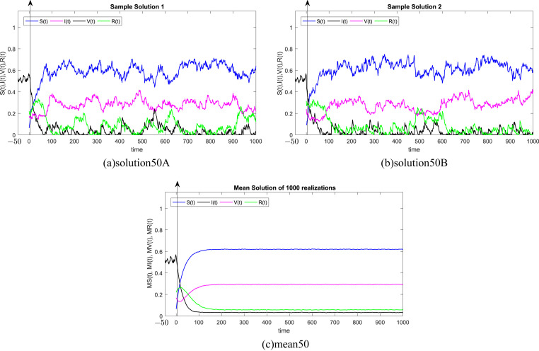
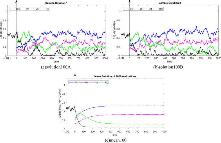
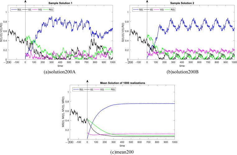
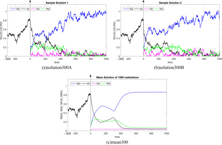
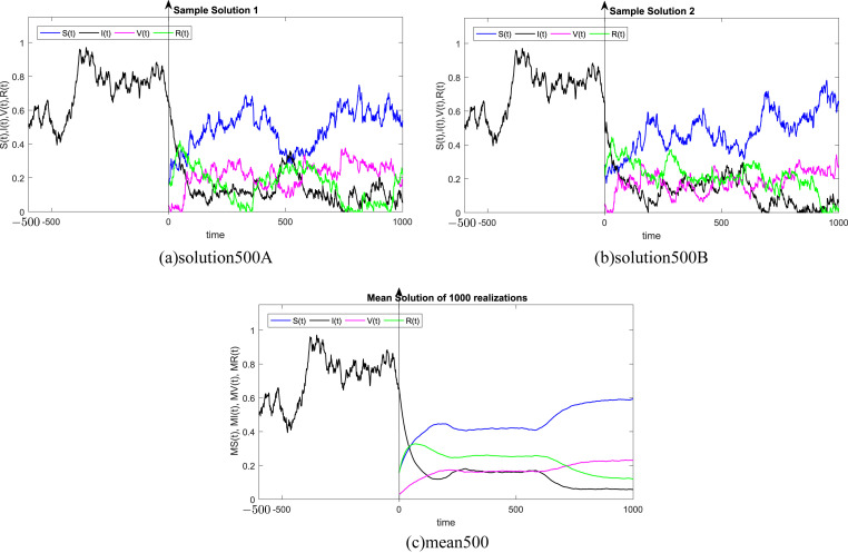
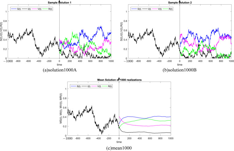
where Δt _n = t _n+1 − t _n represents the non constant time increment and $\mathrm{\Delta }{W}_{i,t_n}=W_{i,t_{n+1}}-W_{i,t_n}$ refers the independent Gaussian Brownian motion increment, for i = 1, 2, 3, 4. In our case, we restrict ourselves to a constant time step Δt _n = Δt. We subdivide the time interval into 1000 equidistant time steps. Where, the delay process I is taken into consideration separately and simulated using different memories τ = 50Δt, 100Δt, 200Δt, 300Δt, 500Δt, 1000Δt. We numerically solve the SIVR system (2) under various random initial conditions satisfying our theoretical results above. It should be stressed, that the delay condition means that the initial value I(0) can not be fixed. Therefore, It takes the end value of the process I starting from I(−τ). The starting values for the individuals S(0), V(0) and R(0) are generated randomly in the interval [0, 1]. Noted that, the system (2) is driven by four independent white noises ΔW _i(t) for i = 1, 2, 3, 4. In order to ensure the first order of our numerical scheme, the multiple stochastic integrals are approximated using the Fourier series. The used parameters are summarized in Table (1) and 1000 realization have been taken for mean simulations. The values of the correlations coefficients σ _i for i = 1, 2, 3, 4 are chosen randomly using the uniform random generator with values in (0, 1). We examine the following six tests:

In all Fig. 1, Fig. 2, Fig. 3, Fig. 4, Fig. 5, Fig. 6 , we present the numerical solution of the SIVR model (2). The two rows from the left show two solutions out of 1000 realizations for the Tests 1–6, while the third column represents the mean solution of the 1000 realizations. Using randomly chosen parameters, we performed short (50Δt and 100Δt) medium (200Δt and 300Δt) and long (500Δt and 1000Δt) memories. The stability of the asymptotic solution is justified for all tests, especially for the short and medium delays. However, for the long delay, we remarked different emerging of the solution. This happens in the transition phase [0, τ]. In addition, it should be stressed that convergence and stability are guaranteed for all tests even for fixed parameters. Finally, based on the simulation Tests 1–6, we remarked that all results satisfy the outcomes of Theorem (1). Namely, (S(t), I(t), V(t), R(t)) exits in ${\mathbb{R}}_{+}^4$ for any on t ≥ − τ, Moreover, all tests show an accurate numerical stability of the SIVR system (2).

Fig. 1.

Simulation of TEST 1.

Fig. 2.

Simulation of TEST 2.

Fig. 3.

Simulation of TEST 3.

Fig. 4.

Simulation of TEST 4.

Fig. 5.

Simulation of TEST 5.

Fig. 6.

Simulation of TEST 6.

Given the deterministic SIVR model (1), if the basic reproduction number $R_0=\frac{\beta }{\mu +\lambda }<1$, then the disease-free equilibrium point is globally asymptotically stable; whereas if R ₀ > 1, the unique endemic equilibrium point is globally asymptotically stable. Repeated outbreaks of the infection can occur due to the time-delay in the transmission terms. In our stochastic SIVR model (2), if $R_0^s=\frac{\phi \rho \beta \mu }{\widehat{\lambda }\widehat{\theta }\widehat{\phi }\widehat{\mu }}<1<R_0$ and $\mu -\frac{{\sigma }_1^2\vee {\sigma }_2^2\vee {\sigma }_3^2\vee {\sigma }_4^2}{2}>0$, the stochastic model (2) has disease extinction with probability one, and for $R_0^s>1$, the model has a unique ergodic stationary distribution.

6. Conclusion

We have reformulated a stochastic epidemic model consisting of four human classes. First of all, we have showed that there exists a unique positive solution to our proposed model. The stochastic basic reproduction number $R_0^s$ has been established. The stationary distribution under several conditions has been obtained by incorporating stochastic Lyapunov function. The extinction for the proposed disease model has been obtained by using the local martingale theorem. The first order stochastic Runge-Kutta scheme is taken into account to depict the numerical simulations. It is derived from our results that the white noise plays a tremendous role in controlling COVID-19; a sufficient large white noise results in the extinction of COVID-19.

Declaration of competing interest

“The authors declare that they have no competing interests.”

References

- 1.Capasso Vincenzo, Serio Gabriella. A generalization of the Kermack-McKendrick deterministic epidemic model. Math. Biosci. 1978;42(1–2):43–61. [Google Scholar]
- 2.Brauer Fred. The Kermack–McKendrick epidemic model revisited. Math. Biosci. 2005;198(2):119–131. doi: 10.1016/j.mbs.2005.07.006. [DOI] [PubMed] [Google Scholar]
- 3.Wang Zhi-Cheng, Wu Jianhong. Travelling waves of a diffusive Kermack–McKendrick epidemic model with non-local delayed transmission. Proc. Math. Phys. Eng. Sci. 2010;466(2113):237–261. [Google Scholar]
- 4.Ovaskainen Otso, Meerson Baruch. Stochastic models of population extinction. Trends Ecol. Evol. 2010;25(11):643–652. doi: 10.1016/j.tree.2010.07.009. [DOI] [PubMed] [Google Scholar]
- 5.Din Anwarud, Khan Amir, Dumitru Baleanu. Stationary distribution and extinction of stochastic coronavirus (COVID-19) epidemic model. Chaos, Solit. Fractals. 2020:110036. doi: 10.1016/j.chaos.2020.110036. [DOI] [PMC free article] [PubMed] [Google Scholar]
- 6.Zhou Y., Zhang W., Yuan S. Survival and stationary distribution of a SIR epidemic model with stochastic perturbations. Appl. Math. Comput. 2014;244:118–131. [Google Scholar]
- 7.El Fatini, Mohamed Idriss Sekkak, Aziz Laaribi. A threshold of a delayed stochastic epidemic model with Crowly–Martin functional response and vaccination. Phys. Stat. Mech. Appl. 2019;520:151–160. [Google Scholar]
- 8.Cao Boqiang, Shan Meijing, Zhang Qimin, Wang Weiming. A stochastic SIS epidemic model with vaccination. Phys. Stat. Mech. Appl. 2017;486:127–143. [Google Scholar]
- 9.Zhao Dianli, Yuan Sanling. Persistence and stability of the disease-free equilibrium in a stochastic epidemic model with imperfect vaccine. Adv. Differ. Equ. 2016;(1):1–14. 2016. [Google Scholar]
- 10.Naik P.A., Yavuz M., Qureshi S., Zu J., Townley S. Modeling and analysis of COVID-19 epidemics with treatment in fractional derivatives using real data from Pakistan. Eur. Phys.J.Plus. 2020;135(10):1–42. doi: 10.1140/epjp/s13360-020-00819-5. [DOI] [PMC free article] [PubMed] [Google Scholar]
- 11.Yavuz M., Coşar F.Ö., Günay F., Özdemir F.N. A new mathematical modeling of the COVID-19 pandemic including the vaccination campaign. Open J. Model. Simulat. 2021;9(3):299–321. [Google Scholar]
- 12.Daşbaşı B. Stability analysis of an incommensurate fractional-order SIR model. Math. Model. Numer. Simulat. Appl. 2021;1(1):44–55. [Google Scholar]
- 13.Özköse F., Yavuz M. Investigation of interactions between COVID-19 and diabetes with hereditary traits using real data: a case study in Turkey. Comput. Biol. Med. 2021;105044 doi: 10.1016/j.compbiomed.2021.105044. [DOI] [PubMed] [Google Scholar]
- 14.Naik P.A., Yavuz M., Zu J. The role of prostitution on HIV transmission with memory: a modeling approach. Alexandria. Eng. J. 2020;59(4):2513–2531. [Google Scholar]
- 15.Uçar E., Uçar S., Evirgen F., Özdemir N. Investigation of E-cigarette smoking model with Mittag-Leffler Kernel. Found. Comput. Decis. Sci. 2021;46(1):97–109. [Google Scholar]
- 16.Jena R.M., Chakraverty S., Yavuz M., Abdeljawad T. A new modeling and existence–uniqueness analysis for Babesiosis disease of fractional order. Mod. Phys. Lett. B. 2021;35(30):2150443. [Google Scholar]
- 17.Bonyah E., Yavuz M., Baleanu D., Kumar S. A robust study on the listeriosis disease by adopting fractal-fractional operators. Alexandria. Eng. J. 2022;61(3):2016–2028. [Google Scholar]
- 18.Kaymak Ö.Ö., Kaymak Y., Özdemir N. Forecasting of the istanbul stock exchange (ISE) return with a golden ratio model in the epidemic of COVID-19. Appl. Comput. Math. 2021;20(1):95–107. [Google Scholar]
- 19.Naik P.A., Owolabi K.M., Yavuz M., Zu J. Chaotic dynamics of a fractional order HIV-1 model involving AIDS-related cancer cells. Chaos, Solit. Fractals. 2020;140:110272. [Google Scholar]
- 20.Hammouch Z., Yavuz M., Özdemir N. Numerical solutions and synchronization of a variable-order fractional chaotic system. Math. Model. Numer. Simulat. Appl. 2021;1(1):11–23. [Google Scholar]
- 21.Allegretti S., Bulai I.M., Marino R., Menandro M.A., Parisi K. Vaccination effect conjoint to fraction of avoided contacts for a Sars-Cov-2 mathematical model. Math. Model. Numer. Simulat. Appl. 2021;1(2):56–66. [Google Scholar]
- 22.Settati A., Lahrouz A., Zahri M., Tridane A., El Fatini M., El Mahjour H., Seaid M. A stochastic threshold to predict extinction and persistence of an epidemic SIRS system with a general incidence rate. Chaos, Solit. Fractals. 2021;144:110690. [Google Scholar]
- 23.Mao X.R. Horwood; New York, NY, USA: 1997. Stochastic Differential Equations and Applications. [Google Scholar]
- 24.Hussain G., Khan A., Zahri Mostafa, Zaman G. Stochastic permanence of an epidemic model with a saturated incidence rate. Chaos, Solit. Fractals. 2020;139(2) [Google Scholar]
- 25.Khan Amir, Hussain Ghulam, Zahri Mostafa, Zaman Gul, Usa Wannasingha Humphries A stochastic SACR epidemic model for HBV transmission. J. Biol. Dynam. 2020;14(1):788–801. doi: 10.1080/17513758.2020.1833993. [DOI] [PubMed] [Google Scholar]
- 26.Khan Tahir, Khan Amir, Zaman Gul. ”The extinction and persistence of the stochastic hepatitis B epidemic model. Chaos, Solit. Fractals. 2018;108:123–128. [Google Scholar]
- 27.Allen Linda JS., Glenn E., Lahodny Extinction thresholds in deterministic and stochastic epidemic models. J. Biol. Dynam. 2012;6(2):590–611. doi: 10.1080/17513758.2012.665502. [DOI] [PubMed] [Google Scholar]
- 28.Song Yi, Miao Anqi, Zhang Tongqian, Wang Xinzeng, Liu Jianxin. Extinction and persistence of a stochastic SIRS epidemic model with saturated incidence rate and transfer from infectious to susceptible. Adv. Differ. Equ. 2018;(1):1–11. 2018. [Google Scholar]
- 29.Kiouach Driss, Sabbar Yassine. Ergodic stationary distribution of a stochastic hepatitis B epidemic model with interval-valued parameters and compensated Poisson process. Comput. Math. Methods . Med. 2020;2020 doi: 10.1155/2020/9676501. [DOI] [PMC free article] [PubMed] [Google Scholar]
- 30.Lv Jingliang, Liu Heng, Zou Xiaoling. Stationary distribution and persistence of a stochastic predator-prey model with a functional response. J. Appl. Anal.Comput. 2019;9(1):1–11. [Google Scholar]