Multilevel Modeling of Spatially Nested Functional Data: Spatiotemporal Patterns of Hospitalization Rates in the U.S. Dialysis Population

Summary

End-stage renal disease patients on dialysis experience frequent hospitalizations. In addition to known temporal patterns of hospitalizations over the life span on dialysis, where poor outcomes are typically exacerbated during the first year on dialysis, variations in hospitalizations among dialysis facilities across the U.S. contribute to spatial variation. Utilizing national data from the United States Renal Data System (USRDS), we propose a novel multilevel spatiotemporal functional model to study spatiotemporal patterns of hospitalization rates among dialysis facilities. Hospitalization rates of dialysis facilities are considered as spatially nested functional data with longitudinal hospitalizations nested in dialysis facilities and dialysis facilities nested in geographic regions. A multilevel Karhunen-Loéve expansion is utilized to model the two-level (facility and region) functional data, where spatial correlations are induced among region-specific principal component scores accounting for regional variation. A new efficient algorithm based on functional principal component analysis and Markov Chain Monte Carlo is proposed for estimation and inference. We report a novel application using USRDS data to characterize spatiotemporal patterns of hospitalization rates for over 400 health service areas across the U.S. and over the post-transition time on dialysis. Finite sample performance of the proposed method is studied through simulations.

1. Introduction

End-stage renal disease (ESRD) affected more than 746,000 individuals in the United States as of 2018 and about 70% of patients were on dialysis, a life-sustaining treatment.¹ Patients on dialysis have a high burden of complex comorbid conditions and patients experience frequent hospitalizations over time, about twice a year on average. Hospitalization is a major contributor to morbidity, mortality, and healthcare cost in the dialysis population. In addition, ESRD patients typically remain on dialysis for the duration of their lives (or until kidney transplantation) and their hospitalization risks change over time after transitioning to dialysis. Indeed, temporal variations in hospitalization rates have been documented, with substantially elevated rates especially in the first year after transition to dialysis.¹ Characterizing hospitalization patterns as a function of time after transitioning to dialysis contributes to understanding of time periods of increased hospitalization risk for more targeted patient monitoring.

In addition to temporal changes, variations in hospitalizations among dialysis facilities across the U.S. contribute to spatial variation. In recent years, efforts to understand spatial patterns of hospitalizations in the U.S. for identification of “hot spot” regions have been recognized by the USRDS.¹ Understanding the geospatial patterns of hospitalizations and other patient outcomes is one of the key national USRDS objectives in annual reporting of the epidemiology of kidney diseases in the U.S. However, current initial efforts to date are largely descriptive, reporting time-static raw or simple adjusted rates by regions (e.g., maps of rates). These approaches (1) do not consider the critical temporal variation after transition to dialysis and (2) cannot model variation among dialysis facilities within regions. Thus, there is a compelling need to develop multilevel spatiotemporal models for hospitalization rates in the dialysis population, where variations across regions and dialysis facilities nested in regions are both estimated.

To address both the aforementioned scientific and methodology gaps in knowledge, we develop a novel multilevel spatiotemporal functional model (MST-FM). MST-FM utilizes multilevel data from the USRDS where longitudinal hospitalizations over time are nested in dialysis facilities and dialysis facilities are nested within geographic regions. Consistent with national reporting standards in this population, we consider the unit for geographic region as health service areas (HSAs), which are regions with relatively self-contained infrastructure for the provision of hospital care. We note that rather than modeling time- and region-aggregated rates directly as a spatiotemporal process to examine hot spots of hospitalizations across the U.S. over time, MST-FM models hospitalization patterns at the facility-level (i.e., using facility-specific rates). This approach is taken to target a more granular estimate of the spatial variation; specifically, variation in hospitalizations among facilities within a region, which is not possible with traditional spatiotemporal analysis with aggregated data at the region level. For instance, a hot spot region could be due to extremely high hospitalization rates from a few facilities or due to consistently high hospitalization rates across a high percentage of the facilities within a region. The proposed MST-FM aims to study these underlying facility-level contribution to spatial variations observed in hospitalization patterns across regions.

Conceptualizing multilevel spatiotemporal data as spatially nested functional data, MST-FM involves multilevel Karhunen-Loève (KL) expansions. Furthermore, to capture spatial dependencies among regions that are complex, such as facility- and region-specific practice patterns and infrastructure, a conditional autoregressive (CAR) structure is induced among region-specific principal component (PC) scores to model region-level correlations.

Our proposed MST-FM is distinct from models proposed in the extensive spatiotemporal modeling literature in the fields of environmental health, criminology, and disease mapping.^2,3 In these developments, the primary interest is prediction, either for time points in the future or for unmeasured spatial locations.^4,5 In contrast, the literature on multilevel spatiotemporal modeling is limited. The few works on multilevel spatiotemporal modeling take a functional data analysis (FDA) approach, although with different goals than prediction, specifically to draw valid multilevel inference accounting for multilevel spatial and temporal correlations and to study spatiotemporal patterns at a granular level.^6–8 The literature on FDA⁹ has seen rapid growth over the past two decades, with a focus on applications to longitudinal data.^10–14 More recent works have considered modeling of structured functional trajectories with spatial or temporal proximity induced dependencies among curves.^6,15–19 Functional variability is typically decomposed via functional principal components analysis (FPCA) using the KL representation. For functional data (FD) that is collected over multiple longitudinal visits, Di et al.¹⁷ proposed decomposing sources of functional variation in an additive fashion via multilevel ANOVA (referred to as multilevel FPCA, MFPCA), with extensions to nonparametric dynamic trends over time.^16,20,21 For spatially correlated multilevel FD, spatial correlations have typically been induced at a lower level in the hierarchy, nested within independent subjects. Examples include electroencephalogram data recorded at electrodes placed on the scalp (spatially correlated) nested within subjects,^22,23 and inhibitor protein measured as a function of the cell positions within the colon crypt (spatially correlated) nested within rats.^6–8

In contrast to previous functional approaches to multilevel spatiotemporal data, we consider spatial correlations at the highest level of the hierarchy (i.e., among regions) motivated by the USRDS data. Spatial correlations at the highest level of the hierarchy pose two unique challenges. First, sample realizations at the highest level are observed only once (without repetition) and hence spatial correlations at this level cannot be handled with nonparametric modeling approaches typically used in FDA. Second, the data structure induces correlations throughout the entire data set (with lack of independent components), leading to the challenge of modeling high-dimensional correlation structures. This hinders estimation of PC scores and therefore best linear unbiased prediction (BLUP) estimation of PC scores becomes infeasible due to inversion of very large covariance matrices. A key innovation here is that our proposed MST-FM incorporates a parametric CAR model into the nonparametric multilevel KL expansions in order to handle spatial correlations at the highest level of the hierarchy, combining a continuous time index, representing time after transition to dialysis, with a discrete spatial dependency structure at the region-level as outlined in Section 2.1. This, to the best of our knowledge, has hitherto remained unexplored. While the CAR model has been considered in the context of basis expansions,⁴ such methods have been proposed for single-level functional data in a parametric setting for modeling spatially correlated genomic changes as a function of genomic location (time) and areal regions of the bladder tissue (space). More critically, the problem/focus in Zhang et al.⁴ did not require addressing the challenges of multilevel spatiotemporal modeling, and therefore did not offer multilevel inference. These are unique challenges faced with spatiotemporal modeling with the USRDS data. Therefore, to address the estimation challenge due to multilevel high-dimensional correlated data, we propose a new efficient algorithm based on FPCA and Markov Chain Monte Carlo (MCMC) methods, in targeting the parameters of the MST-FM. The estimation and multilevel inference tools are outlined in Sections 2.2 and 2.3. Spatiotemporal modeling of hospitalizations using the USRDS data, a national database containing data on nearly all dialysis patients in the U.S., is described in Section 3. Simulation studies are summarized in Section 4, where comparisons of the proposed MST-FM with MFPCA (ignoring spatial correlations) are also included, followed by a discussion in Section 5.

2. The Proposed MST-FM

2.1. Model Specification

Let i = 1, 2, …, n index regions, j = 1, 2, …, N_i index dialysis facilities within the ith region and k = 1, 2, …, T index the kth month after transition to dialysis. The outcome, Y_ijk = Y_ij(t_ijk), denotes the hospitalization rate of the jth facility from region i at time (month) k. This rate is defined as the ratio of the total number of patient hospitalizations to the total patient follow-up time for the jth facility in month k, multiplied by 12 (so that the rate unit can be readily interpreted as a rate per person-year consistent with annual national reporting from the USRDS). For our analysis of the USRDS data in Section 3, we consider region units as HSAs across U.S. and aggregate hospitalization data monthly, for a total of 24 observations per facility over the first two years of follow-up after transitioning to dialysis. Also, for our spatiotemporal approach we opt to model the response as continuous (e.g., via Gaussian spatiotemporal model) similar to previous seminal works⁵ and amenable with the proposed FDA framework.

To study both temporal and spatial variations in hospitalization rates after transition to dialysis and to accommodate the multilevel structure of the data where hospitalization rates over time are nested within facilities and facilities are nested within regions, the proposed MST-FM is given by

$$Y_{ij}(t)=\mu (t)+U_i^{(1)}(t)+U_{ij}^{(2)}(t)+{ϵ}_{ij}(t).$$ (1)

In (1), μ(t) denotes the overall mean hospitalization rate, $U_i^{(1)}(t)$ and $U_{ij}^{(2)}(t)$ denote the first-level (region-level) and second-level (facility-level) deviations from the overall mean, respectively, and ϵ_ij(t) denotes the measurement error. KL expansions are used to decompose both the first- and second-level deviations as:

$$U_i^{(1)}(t)=\sum _{\ell =1}^{\infty }{\xi }_{i\ell }{\psi }_{\ell }^{(1)}(t),U_{ij}^{(2)}(t)=\sum _{m=1}^{\infty }{\zeta }_{ijm}{\psi }_m^{(2)}(t),$$ (2)

where ξ_iℓ and ζ_ijm are the region-level and the facility-level principal component (PC) scores, and ${\psi }_{\ell }^{(1)}(t)$ and ${\psi }_m^{(2)}(t)$ are the region-level and facility-level eigenfunctions, respectively. Under the standard functional principal component analysis (FPCA) framework, eigenfunctions at the first-, $\left\{{\psi }_{\ell }^{(1)}(t),\ell =1,2,\dots \right\}$, and second-level, $\left\{{\psi }_m^{(2)}(t),m=1,2,\dots \right\}$, are assumed to be orthonormal (not necessarily mutually orthogonal across levels) and the PC scores {ξ_iℓ : ℓ = 1, 2, …} and {ζ_ijm : m = 1, 2, …} are assumed to be uncorrelated with zero means and finite variances. In practice, the KL expansions in (2) are truncated to include finite numbers of eigen components, denoted by L (first-level) and M (second-level), which are typically chosen by the fraction of variance explained (FVE).

To capture the spatial correlation among regions, we introduce a conditional autoregressive (CAR) structure on the region-specific PC scores ξ_iℓ. More specifically, suppose that the neighborhood structure of the regions is described by an n × n adjacency matrix W = {w_ii′}, where w_ii′ = 1 if regions i and i′ (i ≠ i′) are neighbors, denoted by i ~ i′, and w_ii′ = 0 otherwise. By convention, the diagonal elements of W are set to zero. Further let D be the diagonal matrix consisting of elements d_i = Σ_i′~i w_ii′, denoting the number of neighbors of region i. A Markov Random Field (MRF) for region units specifies the full conditional distribution for the ℓth PC score for region i, ξ_iℓ, as a weighted average of the ℓth PC scores from neighbors of region i: ξ_iℓ|{ξ_i′ℓ}_i′≠i ~ N (ν Σ_i′~i w_ii′ξ_i′ℓ/d_i, α_ℓ/d_i) with a variance component α_ℓ and a spatial correlation parameter ν. Through Brook’s lemma,^24,25 the joint distribution of the ℓth PC scores ξ_ℓ = (ξ_1ℓ, …, ξ_nℓ)^⊤ takes the form ξ_ℓ ~ N{0, α_ℓ(D−νW)⁻¹}. A sufficient condition for the precision matrix (D − νW)/α_ℓ to be positive definite is when the spatial correlation parameter ν is in (0, 1); see, e.g., the discussion on p82 in Banerjee et al.²⁶ The CAR model can be thought of as a smoother over neighboring regions where spatial information is borrowed across neighbors.

At the second-level, the facility-specific PC scores, ζ_ijm, are assumed to be uncorrelated with E(ζ_ijm) = 0 and var(ζ_ijm) = λ_im, leading to the following covariance structure (C1) between facilities j and j′ from neighboring regions i and i′, (C2) between facilities j and j′ from the same region i (i.e., between facility covariance, denoted by G_Bi(t, t′)) and finally (C3) within facility j from region i (i.e., total facility covariance, denoted by G_Ti(t, t′)):

$$\text{cov}\left\{Y_{ij}(t),Y_{i^{\prime }{j}^{\prime }}\left(t^{\prime }\right)\right\}=\sum _{\ell =1}^L\text{cov}\left({\xi }_{i\ell },{\xi }_{i^{\prime }\ell }\right){\psi }_{\ell }^{(1)}(t){\psi }_{\ell }^{(1)}\left(t^{\prime }\right),$$ (C1)

$$G_{Bi}\left(t,t^{\prime }\right)\equiv \text{cov}\left\{Y_{ij}(t),Y_{i{j}^{\prime }}\left(t^{\prime }\right)\right\}=\sum _{\ell =1}^L\text{var}\left({\xi }_{i\ell }\right){\psi }_{\ell }^{(1)}(t){\psi }_{\ell }^{(1)}\left(t^{\prime }\right),$$ (C2)

$$G_{Ti}\left(t,t^{\prime }\right)\equiv \text{cov}\left\{Y_{ij}(t),Y_{ij}\left(t^{\prime }\right)\right\}=G_{Bi}\left(t,t^{\prime }\right)+G_{Wi}\left(t,t^{\prime }\right),$$ (C3)

where G_Bi(t, t′) and $G_{Wi}\left(t,t^{\prime }\right)={\sum }_{m=1}^M\text{var}\left({\zeta }_{ijm}\right){\psi }_m^{(2)}(t){\psi }_m^{(2)}\left(t^{\prime }\right)$ are between- and within-facility covariance components, respectively. Hence, while first-level dependencies induce spatiotemporal correlation among different facilities within the same region or neighboring regions (C1, C2), the second-level dependencies induce additional temporal correlation within a given facility (C3). In addition, the total facility variance, G_Ti(t, t′), is allowed to vary across regions, partly determined by the neighboring structure (first-level dependencies) and partly by the additional region-specific variation (second-level dependencies) (C3).

While data from all facilities across all regions contribute to estimation of the first- and second-level eigenfunctions, ${\psi }_{\ell }^{(1)}(t)$ and ${\psi }_m^{(2)}(t)$ as well as the first-level PC score variance parameters, only within region data is available to target region-specific variations, var(ζ_ijm) = λ_im at the second-level (in (C3)). To bring stability to region-specific variance estimation, we model the second-level eigenvalues λ_im with two components: ${\lambda }_{im}={\lambda }_m{\tau }_i^2$. Note that the first component λ_m, which is assumed to be the same across regions, satisfies λ₁ ≥ λ₂ ≥ ⋯ ≥ λ_M, ${\sum }_{m=1}^M{\lambda }_m<\infty$, implying that the ordering of the second-level eigencomponents according to FVE and their respective FVE stays the same across regions. The second component ${\tau }_i^2$, which is region-specific, contributes to heterogeneity of variances across regions. Finally, the measurement error ϵ_ij(t)’s are i.i.d with mean zero and variance σ² and are uncorrelated with both region- and facility-specific PC scores.

2.2. Estimation Procedure

The proposed estimation algorithm starts by decomposing the total facility variation within region i, G_Ti(t, t′), into between-facility (G_Bi(t, t′)) and within-facility (G_Wi(t, t′)) covariance components: G_Ti(t, t′) = G_Bi(t, t′) + G_Wi(t, t′) as given in (C3). While the total and between-facility covariances can be targeted directly through the empirical covariances within region i, the within facility covariance is targeted by the difference G_Wi(t, t′) = G_Ti(t, t′) − G_Bi(t, t′). Once the information on between- and within-facility covariances is pooled across regions, FPCA of these pooled covariances leads to the estimation of the first- and second-level eigenfunctions: $\left\{{\psi }_{\ell }^{(1)}(t):\ell =1,2,\dots ,L\right\}$ and $\left\{{\psi }_m^{(2)}(t):m=1,2,\dots ,M\right\}$, respectively. We note that the covariance of facilities across regions (C1) is not used in estimation of the first-level eigenfunctions and that estimation of the eigenfunctions from both levels are restricted to covariances within regions. This apt choice is mainly due to smaller observed between-region covariance relative to within-region variance. Hence, there is limited gain in including covariance of facilities across regions in eigenfunction estimation, but their inclusion would increase the computational cost. After estimation of region-specific eigenvalues λ_im, first-level spatial variance parameters (α_ℓ and ν), measurement error variance (σ²), and region- and facility-specific PC scores (ξ_iℓ and ζ_ijm) are all targeted using MCMC under a mixed effects model framework, using the estimated μ(t), ${\psi }_{\ell }^{(1)}(t)$, ${\psi }_m^{(2)}(t)$ and λ_im. Table 1 outlines the steps of the proposed estimation algorithm, with key details provided below. More specifically, in the first step, a penalized spline smoother is used on the entire data to obtain $\widehat{\mu }(t)$ where the smoothing parameter is selected by generalized cross validation (GCV). The estimated mean is then used to center the observed data, ${\widehat{Y}}_{ij}^c(t)=Y_{ij}(t)-\widehat{\mu }(t)$, leading to the raw estimators of the total and between-facility covariances, ${\widehat{G}}_{Ti}\left(t_k,t_{\ell }\right)={\sum }_{j=1}^{N_i}{\widehat{Y}}_{ij}^c\left(t_k\right){\widehat{Y}}_{ij}^c\left(t_{\ell }\right)/N_i$ and ${\widehat{G}}_{Bi}\left(t_k,t_{\ell }\right)={\sum }_{j=1}^{N_i}{\sum }_{j^{\prime }\ne j}{\widehat{Y}}_{ij}^c\left(t_k\right){\widehat{Y}}_{i{j}^{\prime }}^c\left(t_{\ell }\right)/\left\{N_i\left(N_i-1\right)\right\}$, within region i. The within facility variance is obtained by the difference ${\widehat{G}}_{Wi}\left(t_k,t_{\ell }\right)={\widehat{G}}_{Ti}\left(t_k,t_{\ell }\right)-{\widehat{G}}_{Bi}\left(t_k,t_{\ell }\right)$. Before the FPCA in Step 4, the between and within facility raw covariances are aggregated across regions by averaging, ${\sum }_{i=1}^n{\widehat{G}}_{Bi}\left(t,t^{\prime }\right)/n$ and ${\sum }_{i=1}^n{\widehat{G}}_{Wi}\left(t,t^{\prime }\right)/n$, followed by a two-dimensional penalized spline smoother to obtain the between- and within-facility covariances ${\widehat{G}}_B\left(t,t^{\prime }\right)$ and ${\widehat{G}}_W\left(t,t^{\prime }\right)$.

Table 1:

Main steps of the MST-FM estimation algorithm.

MST-FM Estimation Algorithm
Step 1: Estimate μ(t) by applying a penalized spline smoother to all observed data.
Step 2: Obtain raw estimators of the total variance, ${\widehat{G}}_{Ti}\left(t,t^{\prime }\right)=\widehat{\text{cov}}\left\{Y_{ij}(t),Y_{ij}\left(t^{\prime }\right)\right\}$, and between-facility covariance, ${\widehat{G}}_{Bi}\left(t,t^{\prime }\right)=\widehat{\text{cov}}\left\{Y_{ij}(t),Y_{i{j}^{\prime }}\left(t^{\prime }\right)\right\}$, within region i, directly using empirical covariances. Obtain the raw estimator of within-facility covariance in region i by the difference ${\widehat{G}}_{Wi}\left(t,t^{\prime }\right)={\widehat{G}}_{Ti}\left(t,t^{\prime }\right)-{\widehat{G}}_{Bi}\left(t,t^{\prime }\right)$.
Step 3: Obtain estimators of the between-facility (${\widehat{G}}_B\left(t,t^{\prime }\right)$) and within-facility (${\widehat{G}}_W\left(t,t^{\prime }\right)$) co-variances by smoothing average of between-facility (${\sum }_{i=1}^n{\widehat{G}}_{Bi}\left(t,t^{\prime }\right)/n$) and within-facility (${\sum }_{i=1}^n{\widehat{G}}_{Wi}\left(t,t^{\prime }\right)/n$) raw covariances aggregated across regions.
Step 4: Employ FPCA on ${\widehat{G}}_B\left(t,t^{\prime }\right)$ and ${\widehat{G}}_W\left(t,t^{\prime }\right)$ to get first- and second-level eigenfunction estimators: $\left\{{\widehat{\psi }}_{\ell }^{(1)}(t):\ell =1,2,\dots ,L\right\}$ and $\left\{{\widehat{\psi }}_m^{(2)}(t):m=1,2,\dots ,M\right\}$.
Step 5: Obtain estimators for the region-specific second-level eigenvalues ${\widehat{\lambda }}_{im}^{*}=\iint {\tilde{G}}_{Wi}\left(t,t^{\prime }\right){\widehat{\psi }}_m^{(2)}(t){\widehat{\psi }}_m^{(2)}\left(t^{\prime }\right)dtd{t}^{\prime }$, by projecting the smooth within-facility covariance in region i, denoted by ${\tilde{G}}_{Wi}\left(t,t^{\prime }\right)$, on the second-level eigenfunctions and additional stabilization as detailed below.
Step 6: Estimate the first-level spatial variance parameters (αℓ and v), measurement error variance (σ2) and region- and facility-specific PC scores (ξiℓ and ζijm) by MCMC under the mixed effects modeling framework, using the estimates of μ(t), ${\psi }_{\ell }^{(1)}(t)$, ${\psi }_m^{(2)}(t)$ and λim.

Note that the within-facility covariance function, ${\widehat{G}}_W\left(t,t^{\prime }\right)$, is based on the raw within-facility covariances across regions, obtained as a difference between the total and between-facility raw covariances, and hence may not be positive definite. To obtain a positive definite within-facility covariance estimator, the within-facility covariance is reconstructed using only the eigencomponents with positive eigenvalues.²⁷ In addition, the diagonal entries of ${\sum }_{i=1}^n{\widehat{G}}_{Wi}\left(t,t^{\prime }\right)/n$, which are prone to measurement error, are left out before the two dimensional smoothing is applied to yield ${\widehat{G}}_W\left(t,t^{\prime }\right)$. The diagonal entries of ${\widehat{G}}_{Wi}\left(t,t^{\prime }\right)$ are similarly left out before smoothing in obtaining ${\tilde{G}}_{Wi}\left(t,t^{\prime }\right)$ in Step 5.

For the bivariate penalized spline smoothers used in estimation of the covariance operators, smoothing parameters are selected by restricted maximum likelihood (REML), as proposed by Goldsmith et al.²⁸ Once the between- and within-facility covariances are obtained, first- and second-level eigenfunction estimators: $\left\{{\widehat{\psi }}_{\ell }^{(1)}(t):\ell =1,2,\dots ,L\right\}$ and $\left\{{\widehat{\psi }}_m^{(2)}(t):m=1,2,\dots ,M\right\}$ are recovered by FPCA (Step 4). The number of eigencomponents kept is determined by the FVE. We use FVE > 80% in numerical applications. While the FVE for the region-specific first-level eigencomponents are estimated based on FPCA employed on ${\widehat{G}}_B\left(t,t^{\prime }\right)$, the FVE for the facility-specific second-level eigencomponents are estimated based on FPCA employed on ${\widehat{G}}_W\left(t,t^{\prime }\right)$.

The region-specific second-level eigenvalues are estimated via the projection, ${\widehat{\lambda }}_{im}^{*}=\iint {\tilde{G}}_{Wi}\left(t,t^{\prime }\right){\widehat{\psi }}_m^{(2)}(t){\widehat{\psi }}_m^{(2)}\left(t^{\prime }\right)dtd{t}^{\prime }$, where ${\tilde{G}}_{Wi}\left(t,t^{\prime }\right)$ is obtained by applying a two dimensional smoother to ${\widehat{G}}_{Wi}\left(t,t^{\prime }\right)$. Since only within-region data is available to target region-specific variations, we further stabilize these estimates by ${\widehat{\lambda }}_{im}={\Lambda }_m{\sum }_{m=1}^M\left({\widehat{\lambda }}_{im}^{*}/{\Lambda }_m\right)/M$, where {Λ_m : m = 1, 2, …, M} are the eigenvalues obtained from the FPCA decomposition of ${\widehat{G}}_W\left(t,t^{\prime }\right)$. In our application to the USRDS data, ${\widehat{\lambda }}_{im}$ estimates for three of 423 regions were negative, and thus were set to a small positive number 10⁻⁶. The proposed form for ${\widehat{\lambda }}_{im}$ takes advantage of the assumption that the ordering of the second-level eigenvalues according to the FVE and their respective FVE stays the same across regions and hence estimates {Λ_m : m = 1, 2, …, M} based on the FPCA decomposition of ${\widehat{G}}_W\left(t,t^{\prime }\right)$.

In the final step 6, the first-level spatial parameters (α_ℓ and ν), measurement error variance (σ²) and region- and facility-specific PC scores (ξ_iℓ and ζ_ijm) are targeted by MCMC using a mixed effects modeling framework where the estimate $\widehat{\theta }=\left\{\widehat{\mu }(t),{\widehat{\psi }}_{\ell }^{(1)}(t),{\widehat{\psi }}_m^{(2)}(t),{\widehat{\lambda }}_{im},L,M\right\}$ from previous steps are kept fixed. For estimation of the PC scores, we assume that the scores are independent of the measurement error where both are normally distributed (similar to Yao et al.²⁷ and Di et al.¹⁷). Next, the posterior distributions of the spatial parameters, measurement error variance, and PC scores can then be obtained using MCMC sampling. With inverse Gamma (IG) priors for variance components α_ℓ and σ² and Beta priors for the spatial correlation parameter ν, the model can be rewritten as follows:

$$Y_{ij}\left(t_k\right)=\mu \left(t_k\right)+\sum _{\ell =1}^L{\xi }_{i\ell }{\psi }_{\ell }^{(1)}\left(t_k\right)+\sum _{m=1}^M{\zeta }_{ijm}{\psi }_m^{(2)}\left(t_k\right)+{ϵ}_{ij}\left(t_k\right),$$

$${\xi }_{\ell }~N\left(0,{\alpha }_{\ell }{(D-\nu W)}^{-1}\right),{\zeta }_{ijm}~N\left(0,{\lambda }_{im}\right),{ϵ}_{ij}\left(t_k\right)~N\left(0,{\sigma }^2\right),$$

$${\alpha }_{\ell }~\text{IG}\left(a_{{\alpha }_{\ell }},b_{{\alpha }_{\ell }}\right),{\sigma }^2~\text{IG}\left(a_{{\sigma }^2},b_{{\sigma }^2}\right),\nu ~\text{Beta}\left(a_{\nu },b_{\nu }\right).$$

A Gibbs sampler is used to sample from the posterior distributions of PC scores and the variance components where the full conditional distributions are: ${\xi }_{i\ell }\mid \text{ others }~N\left({\mu }_{\xi ,i\ell }^{\mathit{\text{post}}},v_{\xi ,i\ell }^{\mathit{\text{post}}}\right)$, ${\zeta }_{ijm}\mid \text{ others }~N\left({\mu }_{\zeta ,ijm}^{\mathit{\text{post}}},v_{\zeta ,ijm}^{\mathit{\text{post}}}\right)$, ${\alpha }_{\ell }\mid \text{ others }~IG\left(a_{{\alpha }_{\ell }}^{\mathit{\text{post}}},b_{{\alpha }_{\ell }}^{\mathit{\text{post}}}\right)$ and ${\sigma }^2\mid \text{ others }~IG\left(a_{{\sigma }^2}^{\mathit{\text{post}}},b_{{\sigma }^2}^{\mathit{\text{post}}}\right)$. The above forms specify the conditional posterior distribution of each parameter, conditioning on $\widehat{\theta }$ and the entire MCMC parameter set {ξ_iℓ, ζ_ijm, α_ℓ, σ², ν} and excluding only the parameter whose conditional distribution is sought after (referred to as “others”). The posterior distribution of the spatial correlation parameter, ν, does not have a closed form, and hence ν is updated using a Metropolis approach. Details of the posterior distributions and the sampling methods are deferred to Supporting Information Appendix A.

In order to aid in the inference for the multilevel trajectories proposed in the next section, the MCMC samples drawn from the posterior distributions of the PC scores specified above lead to the estimated first- and second-level PC scores as ${\widehat{\xi }}_{i\ell }=E\left({\xi }_{i\ell }\mid Y,\widehat{\theta }\right)$ and ${\widehat{\zeta }}_{ijm}=E\left({\zeta }_{ijm}\mid Y,\widehat{\theta }\right)$, respectively. These are obtained as the mean of the MCMC samples, where Y = {Y_ijk : i = 1, …, n, j = 1, …, N_i, k = 1, …, T}. Note that since facilities from different regions are correlated through the spatial dependence of the region-specific PC scores, the conditional expectations of region- and facility-level PC scores for facility j in region i does not depend on data only from facility j or region i but depends on the entire dataset, denoted by Y. In addition, the posterior variances of the first-level and second-level PC scores and their covariance, denoted by ${\widehat{\Omega }}_{L\times L}^{(1)}=\text{Var}\left({\xi }_i\mid Y,\widehat{\theta }\right)$, ${\widehat{\Omega }}_{M\times M}^{(2)}=\text{Var}\left({\zeta }_{ij}\mid Y,\widehat{\theta }\right)$ and ${\widehat{\Omega }}_{L\times M}^{(1,2)}=\text{cov}\left({\xi }_i,{\zeta }_{ij}\mid Y,\widehat{\theta }\right)$, respectively, are also estimated from the MCMC samples, where ${\widehat{\xi }}_i={\left({\widehat{\xi }}_{i1},\dots ,{\widehat{\xi }}_{iL}\right)}^{\top }$ and ${\widehat{\zeta }}_{ij}={\left({\widehat{\zeta }}_{ij1},\dots ,{\widehat{\zeta }}_{ijM}\right)}^{\top }$.

2.3. Inference for Multilevel Trajectories

The multilevel structure of the MST-FM enables us to draw inference on hospitalization rate trajectories at both the region and facility levels. The estimation of region- and facility-specific PC scores described in Section 2.2 leads to prediction of the region- and facility-specific trajectories:

$${\widehat{Y}}_i(t)=E\left\{Y_i(t)\mid {\widehat{\xi }}_i,\widehat{\theta }\right\}=\widehat{\mu }(t)+\sum _{\ell =1}^L{\widehat{\xi }}_{i\ell }{\widehat{\psi }}_{\ell }^{(1)}(t)$$ (3)

$${\widehat{Y}}_{ij}(t)=E\left\{Y_{ij}(t)\mid {\widehat{\xi }}_i,{\widehat{\zeta }}_{ij},\widehat{\theta }\right\}=\widehat{\mu }(t)+\sum _{\ell =1}^L{\widehat{\xi }}_{i\ell }{\widehat{\psi }}_{\ell }^{(1)}(t)+\sum _{m=1}^M{\widehat{\zeta }}_{ijm}{\widehat{\psi }}_m^{(2)}(t).$$

In addition, using the posterior variances of the region-specific and facility-specific PC scores and their covariance, the covariances of the predicted trajectories are given by

$$\text{Var}\left\{{\widehat{Y}}_i(t)-Y_i(t)\mid \widehat{\theta }\right\}\approx {\widehat{\Psi }}^{(1)\top }{\widehat{\Omega }}^{(1)}{\widehat{\Psi }}^{(1)},\text{ Var}\left\{{\widehat{Y}}_{ij}(t)-Y_{ij}(t)\mid \widehat{\theta }\right\}\approx {\widehat{\Psi }}^{\top }\widehat{\Omega }\widehat{\Psi },$$

where ${\widehat{\Psi }}^{(1)}={\left\{{\widehat{\psi }}_1^{(1)}(t),\dots ,{\widehat{\psi }}_L^{(1)}(t)\right\}}^{\top }$, $\widehat{\Psi }={\left\{{\widehat{\psi }}_1^{(1)}(t),\dots ,{\widehat{\psi }}_L^{(1)}(t),{\widehat{\psi }}_1^{(2)}(t),\dots ,{\widehat{\psi }}_M^{(2)}(t)\right\}}^{\top }$ and ${\widehat{\Omega }}_{(L+M)\times (L+M)}=\left[{\widehat{\Omega }}^{(1)},{\widehat{\Omega }}^{(1,2)};{\widehat{\Omega }}^{(1,2)\top },{\widehat{\Omega }}^{(2)}\right]$. Next, the approximate (1 − α) pointwise confidence intervals (CIs) for the predicted region- and facility-specific trajectories are given by

$${\widehat{Y}}_i(t)\pm {\Phi }^{-1}\left(1-\frac{\alpha }{2}\right)\sqrt{\text{diag}\left[\text{Var}\left\{{\widehat{Y}}_i(t)-Y_i(t)\mid \widehat{\theta }\right\}\right]},$$

$${\widehat{Y}}_{ij}(t)\pm {\Phi }^{-1}\left(1-\frac{\alpha }{2}\right)\sqrt{\text{diag}\left[\text{Var}\left\{{\widehat{Y}}_{ij}(t)-Y_{ij}(t)\mid \widehat{\theta }\right\}\right]},$$

respectively, where Φ(·) denotes the Gaussian cumulative distribution function.

Note that the above formulation for approximate CIs of the predicted multilevel trajectories relies on effective estimation of the FPCA model parameters θ. While second-level facility-specific parameters are usually well estimated since there are adequate repetitions and stabilization across facilities, the first-level region-specific parameters may be more difficult to estimate for applications with a small number of regions (e.g., when region units are states). The dependence of the predicted trajectories on accurate estimation of the FPCA components for single-level functional data have been recognized in the FDA literature.^27,28 For single-level functional data, Yao et al.²⁷ proposed prediction of subject-specific trajectories based on the BLUP estimators of the PC scores in a mixed effects modeling framework, conditional on the estimated mean function and eigencomponents. Goldsmith et al.²⁸ point out that while this classical construction takes into account model based uncertainty, it does not take into account of the FPCA based uncertainty. Especially in applications with small sample sizes where the uncertainty in the FPCA decomposition is high, the CI construction conditional on the estimated FPCA components may lead to underestimation of the total variability in the predicted subject-specific curves.²⁸ Hence, Goldsmith et al.²⁸ proposed corrected CIs for subject-specific trajectories for single-level functional data that also incorporate decomposition-based uncertainty captured by a bootstrap procedure.

Following Goldsmith et al.,²⁸ we also propose corrected inference for region-specific hospitalization trajectories. While Goldsmith et al.²⁸ uses nonparametric bootstrap, resampling from subjects with replacement, we rely on parametric bootstrap methods in order to preserve the neighboring structure between the regions in the bootstrap samples. The parametric bootstrap samples Y_b are generated based on parameter estimates, $\left\{\widehat{\mu }(t),{\widehat{\psi }}_{\ell }^{(1)}(t),{\widehat{\psi }}_m^{(2)}(t),{\widehat{\lambda }}_{im},{\widehat{\alpha }}_{\ell },\widehat{\nu },{\widehat{\sigma }}^2,L,M\right\}$, obtained from Section 2.2. More specifically, $Y_{ij,b}(t)=\widehat{\mu }(t)+{\sum }_{\ell =1}^L{\xi }_{i\ell ,b}{\widehat{\psi }}_{\ell }^{(1)}(t)+{\sum }_{m=1}^M{\zeta }_{ijm,b}{\widehat{\psi }}_m^{(2)}(t)+{ϵ}_{ij,b}(t)$, where ξ_ℓ,b = (ξ_1ℓ,b, …, ξ_nℓ,b)^⊤ is generated from $N\left\{\mathbf{0},{\widehat{\alpha }}_{\ell }{\left(D-\widehat{\nu }W\right)}^{-1}\right\}$, ζ_ijm,b is generated from $N\left(0,{\widehat{\lambda }}_{im}\right)$ and ϵ_ij,b(t) is generated from $N\left(0,{\widehat{\sigma }}^2\right)$. Next, the multilevel FPCA decomposition based parameters ${\widehat{\theta }}_b=\left\{{\widehat{\mu }}_b(t),{\widehat{\psi }}_{\ell ,b}^{(1)}(t),{\widehat{\psi }}_{m,b}^{(2)}(t),{\widehat{\lambda }}_{im,b},L_b,M_b\right\}$ are estimated based on the bootstrap data Y_b as described in Section 2.2. Conditioning on ${\widehat{\theta }}_b$, we obtain bootstrap estimates of the first-level region-specific PC scores, ${\widehat{\xi }}_{i\ell ,b}$, (via posterior mean of the MCMC samples), region-specific trajectories, ${\widehat{Y}}_{i,b}(t)={\widehat{\mu }}_b(t)+{\sum }_{\ell =1}^{L_b}{\widehat{\xi }}_{i\ell ,b}{\widehat{\psi }}_{\ell ,b}^{(1)}(t)$ and $\text{Var}\left\{{\widehat{Y}}_{i,b}(t)-Y_i(t)\mid {\widehat{\theta }}_b\right\}={\widehat{\Psi }}_b^{(1)\top }{\widehat{\Omega }}_b^{(1)}{\widehat{\Psi }}_b^{(1)}$, where ${\widehat{\Psi }}_b^{(1)}={\left\{{\widehat{\psi }}_{1,b}^{(1)}(t),\dots ,{\widehat{\psi }}_{L_b}^{(1)}(t)\right\}}^{\top }$ and ${\widehat{\Omega }}_b^{(1)}=\text{Var}\left({\xi }_{i,b}\mid Y,{\widehat{\theta }}_b\right)$. The MCMC samples used in obtaining the region-specific PC estimates, ${\widehat{\xi }}_{i\ell ,b}$, and their associated variation, $\text{Var}\left({\xi }_{i,b}\mid Y,{\widehat{\theta }}_b\right)$, condition on the original data Y instead of Y_b, and ${\widehat{\theta }}_b$, since the bootstrap resampling is used only to assess variability in the FPCA decompositions.

Next, information across bootstrap samples are pooled to target region-specific trajectory predictions and adjusted variance that account for variability in the FPCA decompositions, leading to the corrected CIs for region-specific inference. The region-specific trajectory predictions are obtained using iterative expectations: ${\widehat{Y}}_i^c(t)=E_{\widehat{\theta }}\left[E_{Y\mid \widehat{\theta }}\left\{Y_i(t)\mid {\widehat{\xi }}_i,\widehat{\theta }\right\}\right]$, where superscript c denotes quantities of “corrected” inference. The predicted curves are the mean of model-based estimates given in (3) taken over the distribution of the estimated decomposition parameters in $\widehat{\theta }$. Thus, the predicted curves are estimated as averages of ${\widehat{Y}}_{i,b}(t)$ across bootstrap samples. The variance of the predicted curves is given, based on iterative variance, as the sum of the expectation of model-based decomposition variance and the variance of the model-based decomposition expectations:

$$\text{Var}\left\{{\widehat{Y}}_i^c(t)-Y_i(t)\right\}=E_{\widehat{\theta }}\left[{\text{Var}}_{Y\mid \widehat{\theta }}\left\{{\widehat{Y}}_i(t)-Y_i(t)\mid \widehat{\theta }\right\}\right]+{\text{Var}}_{\widehat{\theta }}\left[E_{Y\mid \widehat{\theta }}\left\{{\widehat{Y}}_i(t)-Y_i(t)\mid \widehat{\theta }\right\}\right].$$

While model-based decomposition variance and expectations are estimated separately for each bootstrap sample via $\text{Var}\left\{{\widehat{Y}}_{i,b}(t)-Y_i(t)\mid {\widehat{\theta }}_b\right\}$ and $\left\{{\widehat{Y}}_{i,b}(t)-{\widehat{Y}}_i(t)\right\}$, respectively, the outer expectation and variances are taken over the distribution of the estimated decomposition parameters in $\widehat{\theta }$; hence, the average of $\text{Var}\left\{{\widehat{Y}}_{i,b}(t)-Y_i(t)\mid {\widehat{\theta }}_b\right\}$ and the variance of $\left\{{\widehat{Y}}_{i,b}(t)-{\widehat{Y}}_i(t)\right\}$ are taken over all bootstrap samples. The corrected (1 − α) pointwise CI for the predicted region-level trajectory is given by ${\widehat{Y}}_i^c(t)\pm {\Phi }^{-1}(1-\alpha /2)\times {\left(\text{diag}\left[\text{Var}\left\{{\widehat{Y}}_i^c(t)-Y_i(t)\right\}\right]\right)}^{1/2}$. The proposed algorithm for multilevel trajectory prediction, including the corrected inference for region-specific trajectory prediction is summarized in Supporting Information Appendix B Table S1.

3. Data Analysis

3.1. Description of the USRDS Study Population

The United States Renal Data System collects data on nearly all patients with ESRD in the U.S. Our study cohort includes patients of age 18 years or older who transitioned to dialysis between January 1, 2005 and September 30, 2013. The observation period starts from day 91 of dialysis (after a 90-day period to establish stable treatment modality) and patients are followed up for two years where the last date of follow up is December 31, 2015. Facility hospitalization rates per person-year are calculated monthly over the two years of follow up, with a mean hospitalization rate of 1.8 per person-year. Consistent with national annual USRDS reporting, our analysis consider the region units as HSAs. Also, some HSAs are merged to guarantee that each resulting region contains at least 4 facilities, the minimum number we found to lead to stable region-specific inference. The final study cohort contains 5,494 facilities and 423 regions/HSAs after merging. Detailed descriptions of the study cohort, exclusion rules, and the region merging algorithm are deferred to Supporting Information Appendix C.

3.2. Results

3.2.1. Estimated FPCA Decomposition Components

Figure 1(a) displays the decreasing estimated overall mean hospitalization rate over the first two years on dialysis treatment, with a gradually slower decreasing rate after the first ~10–12 months. The highest hospitalization rate of over 2.1 hospitalizations per person-year is estimated at the start of dialysis transition. The leading eigenfunction, explaining 96.8% of the region-level variation, is given in Figure 1(b). The magnitude of the leading eigenfunction is decreasing over time, with a more rapid decrease in the first ~10 months on dialysis, indicating that the largest variation in hospitalization rates among regions are observed within the first ~10 months of dialysis. The estimated higher hospitalization rates and variability within the first ~10 months of dialysis is consistent with the known fragile one-year period after transitioning to dialysis with high mortality.²⁹

Figure 1:

(a) Estimated overall mean hospitalization rate per person-year. (b) Leading region-level eigenfunction with 96.82% fraction variation explained (FVE). (c-e) First, second, and third leading facility-level eigenfunctions with 72.35%, 10.70%, and 5.17% FVE, respectively.

Figures 1(c)–(e) display the three leading facility-level eigenfunctions, explaining in total more than 88% of the facility-level variation. The leading facility-level eigenfunction with 72.4% FVE is relatively flat, indicating that the most common direction of variation across facilities is constant over time. The FVE drops drastically for the second and third leading eigenfunctions, where the second leading eigenfunction with 10.7% FVE highlights variation at initiation of dialysis and towards the end of the two-year follow up. The third leading eigenfunction with 5.2% FVE highlights variation also near the one year post-dialysis transition in addition to the end of two-year follow up. Thus, variation in hospitalization rates at the initiation of dialysis is not only captured at the region-level, but is found to also contribute to explained variation across facilities, although with a much lower FVE (i.e., through the second and third facility-level eigenfunctions). Note that the higher variation identified at the end of the two year follow up may be due to the decrease in the total number of patients towards the end of the two year follow up.

3.2.2. Predicted Hospitalization Rates

Next, the leading region-level and the three leading facility-level eigenfunctions summarized above are used in multilevel inference for hospitalization rates at the region- and facility-levels. We begin by studying the region-specific predictions. The raw and predicted region-specific hospitalization rates from 1st, 12th and 24th months on dialysis are displayed for all HSAs in Figure 2. While the predicted maps correspond closely to the raw maps of region- and month-specific hospitalization rates, they smooth out the predictions over space as illustrated in Figure 2 (right column). The estimated spatial correlation parameter is $\widehat{\nu }=0.98$, leading to correlations between neighboring HSAs ranging from 0.38 to 0.8. Both raw and estimated maps show a pattern (“band”) of particularly high hospitalization rates from Massachusetts to southern Texas (dark blue), as well as many HSAs in Nevada, Arizona and Florida. In addition, as observed in the estimated overall mean function, displayed in Figure 1(a), the rates are highest in the early months after transitioning to dialysis, with an overall decreasing trend in almost all HSAs throughout the two-year follow up. This change over time can be seen more clearly with the video clip of the predicted region rates available in Supporting Information (HospMapVideo.mp4).

Figure 2:

Raw (left column) and predicted (right column) region-specific hospitalization rates at the 1st, 12th and 24th months after initiation of dialysis for 423 health service areas.

For a more detailed examination of the distribution of the region-specific rate predictions, Table 2 displays the 5th and 95th percentiles and median values of the predicted region-specific hospitalization rates at month 1, 12, and 24 for the West (49 HSAs), Midwest (124 HSAs), Southwest (46 HSAs), Southeast (150 HSAs), and Northeast (54 HSAs) zones of the U.S. Shortly after transitioning to dialysis at month 1, the highest median predicted hospitalization rates are in the Southeast and Northeast with 2.14 and 2.32 per person-year (PPY), respectively, which are 3.4% and 12% higher than the overall median across all HSAs (2.07 PPY). We note that HSAs in the Northeast and Southeast comprise many of the HSAs observed in the band of elevated hospitalizations from Massachusetts to southern Texas in Figure 2. In contrast, the West had the lowest median predicted rate of 1.7 PPY, which is nearly 18% lower than the overall median rate. At the 5th percentile, the predicted hospitalization rate is 27.6% lower in the West (1.34 PPY) compared the Northeast (1.85 PPY). Also, as illustrated in Figure 2, there is an overall decrease in hospitalization rate over time as the population stabilizes. Indeed, from Table 2, the median predicted hospitalization rates from month 1 to month 24 declined by about 0.41 to 0.49 PPY across the five zones, which represent about a 20.2% decline (19.4%, 19.9%, 20.2%, 20.6%, and 21.1% decline from month 1 to 24 for the West, Midwest, Southwest, Southeast, and Northeast, respectively).

Table 2:

The 5th, 50th and 95th percentiles of the predicted region-specific hospitalization rates (with standard errors in the parentheses) across the health service areas (HSAs)/regions of the five U.S. zones (West, Midwest, Southwest, Southeast and Northeast) and overall (all HSAs) at month 1, 12, and 24.

Month	Percentile	Overall	West	Midwest	Southwest	Southeast	Northeast
	5	1.49 (.15)	1.34 (.08)	1.48 (.13)	1.74 (.12)	1.74 (.10)	1.85 (.08)
1	50	2.07 (.13)	1.70 (.12)	2.06 (.15)	2.03 (.10)	2.14 (.13)	2.32 (.14)
	95	2.65 (.09)	2.07 (.09)	2.70 (.07)	2.42 (.06)	2.62 (.14)	2.69 (.07)
	5	1.26 (.12)	1.13 (.06)	1.25 (.10)	1.45 (.09)	1.45 (.08)	1.54 (.06)
12	50	1.72 (.10)	1.42 (.10)	1.72 (.11)	1.68 (.08)	1.78 (.09)	1.92 (.11)
	95	2.18 (.07)	1.72 (.07)	2.22 (.05)	1.99 (.05)	2.16 (.11)	2.21 (.06)
	5	1.22 (.11)	1.11 (.06)	1.21 (.09)	1.40 (.09)	1.40 (.07)	1.48 (.06)
24	50	1.65 (.09)	1.37 (.09)	1.65 (.10)	1.62 (.07)	1.70 (.10)	1.83 (.10)
	95	2.08 (.06)	1.65 (.06)	2.12 (.05)	1.90 (.05)	2.06 (.10)	2.11 (.05)

Figure 3(d) displays the overall predicted region-specific hospitalization trajectories over the full 24 months along with approximate 95% CIs for the West and Northeast zones, as well as results stratified by (a) small (< 7 facilities), (b) medium (7 − 10 facilities), and (c) large (> 10 facilities) regions/HSAs. The decreasing hospitalization patterns over time, overall and across HSAs sizes, is apparent. (Similar patterns were observed in the other geographic zones; results not shown.) The approximate 95% CIs for the region prediction trajectories from the West and Northeast do not overlap for all HSA sizes, indicating that HSAs in the West have consistently lower hospitalizations over time compared to those in the Northeast. (We note that the reported CIs for large regions are narrower, as expected.)

Figure 3:

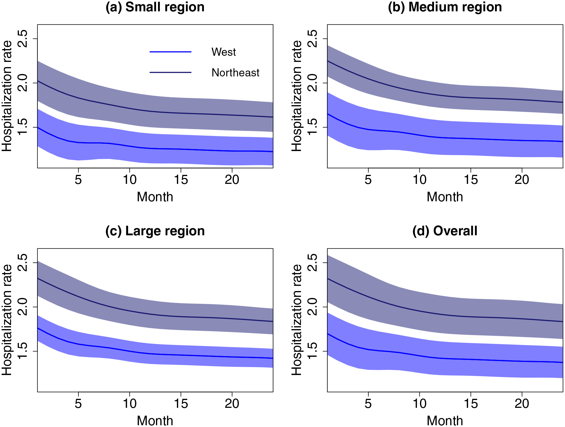
Predicted region-specific trajectories for regions (health service areas [HSAs]) with median hospitalization rates from the West (blue) and Northeast (dark blue) zones, stratified by HSA size: (a) small (< 7 facilities), (b) medium (7 to 10 facilities), and (c) large (> 10 facilities). Also given is the overall trajectories for all HSAs (d). The approximate 95% CIs are given as shaded areas.

Next, for facility-specific inference, Figure 4 displays predicted facility-specific hospitalization rate trajectories, along with their approximate 95% CIs, for facilities from large regions within the five selected major areas: (a) Los Angeles and Orange counties in California from the West, (b) Cook, Lake, McHenry and Dupage counties in Illinois (containing Chicago) from the Midwest, (c) Maricopa, Coconino, Gila, Yavapai and Pinal counties in Arizona (containing Phoenix) from the Southwest, (d) Fulton, Clayton, Dekalb, Fayette, Forsyth, Gwinnett, Henry, Rockdale, Walton, Newton and Jasper counties in Georgia (containing Atlanta) from the Southeast, and (e) Kings, Bronx, Richmond, New York and Queens counties in New York State from the Northeast. The predicted trajectories for facilities with the highest, median and lowest averaged hospitalization rates from each region are depicted, where predictions (solid) correspond to smoothed observed facility-specific hospitalization rates (dashed). Note that facility-specific predictions are more variable in larger regions in (a), (b) and (e) (containing Los Angeles, Chicago and New York, respectively), compared to smaller regions in (c) and (d) (containing Phoenix and Atlanta, respectively), as expected.

Figure 4:

Observed (dashed) and predicted (solid) hospitalization rate trajectories, along with their approximate 95% CIs, for facilities from large regions in five selected areas. Facilities with the highest (dark blue), median (blue), and lowest (light blue) averaged hospitalization rates from five selected areas are depicted.

This relates to the estimation of the region-specific variations λ_im, modeled in the MST-FM, via the two components λ_m and ${\tau }_i^2$. While λ_m is assumed to be the same across regions to stabilize region-specific variance estimation, ${\tau }_i^2$ is region-specific and models the heterogeneity in variances across regions. More specifically, Supporting Information Appendix D Figure S1 (a) displays the map of the raw variances of hospitalization rates across facilities (averaged over time) for each region, while (b) displays the map of the estimated ${\tau }_i^2$. Since the raw variances and ${\tau }_i^2$ are not expected to match in magnitude, they should be compared in relative magnitude, where the breakpoints of the coloring scheme in both maps correspond to the 20th, 40th, 60th and 80th percentiles. Figure S1 shows that the estimated ${\tau }_i^2$ is able to capture the relative heterogeneity in observed region-specific hospitalization rates. In addition, all five selected areas displayed in Figure 4 are found to have high ${\tau }_i^2$ (above .32), indicating that facility-level variations are in general higher in large regions.

4. Simulation Studies

Simulation studies are conducted to examine the finite sample properties of the proposed estimation algorithm for model parameters and inference for the multilevel predictions, under varying error variance, total number of regions and total number of facilities per region. We defer details on simulation design to Appendix E of the Supporting Information and outline simulation results below.

We utilize the relative mean squared deviation error (MSDE), i.e., ${\text{MSDE}}_{\widehat{f}}=\left[\int {\left\{\widehat{f}(t)-f(t)\right\}}^{2}dt\right]/\int f^2(t)dt$ for a generic function f(t), and mean squared error (MSE) to assess estimation of the time-varying and time-invariant parameters, respectively. Note that for region-specific variance estimation, we assess estimation of ${\lambda }_{im}={\lambda }_m{\tau }_i^2$ directly, since λ_m and ${\tau }_i^2$ are not identifiable individually. The results are presented for 8 simulation settings with (a) two error variances σ² = .02 and .2; (b) two total number of regions: n = 423 (similar to HSAs in the USRDS data) and n = 49 (similar to analysis utilizing the contiguous U.S. and D.C. as regions); and (c) two ranges of the number of facilities per region of 4 − 20 and 10 − 30. Reported results are based on 200 Monte Carlo runs, where for each run, 2500 iterations (500 for burn-in and 2000 for estimation and inference) are used in the MCMC step. The Markov chains are verified to have good mixing and convergence properties. More details can be found in Supporting Information Appendix F. Figures S2 and S3 (Appendix F of Supporting Information) display the estimated mean function and eigenfunctions from runs with the 5th, 50th and 95th percentile MSDEs, from the set-up with 423 and 49 regions with number of facilities per region varying from 4 to 20 and σ² = .2. The estimates track the true functions, indicating that the proposed estimation effectively identifies multilevel variations, where the first-level region-specific eigenfunctions, ${\psi }_1^{(1)}(t)$ and ${\psi }_2^{(1)}(t)$, are estimated better, as expected, with increasing number of regions. (Compare Figure S2 and S3.)

The mean MSDE and MSE values from all eight simulation set-ups are reported in Table 3. As expected, error measures for all model parameters get smaller with decreasing noise level σ². Similarly, all error measures, except MSE of region-specific eigenvalues λ_im, decrease with increasing number of regions. This is expected, since estimation of λ_im largely relies on region-specific information; hence, MSE for λ_im gets smaller with increasing total number of facilities per region and by region size (larger regions have smaller λ_im MSEs). Finally, increasing total number of facilities per region also lead to decreasing MSDE for second-level eigenfuncions ${\widehat{\psi }}_m^{(2)}(t)$ and MSE for facility-specific PC scores ζ_ijm, since they yield more regionspecific information for estimation of the second-level decomposition components.

Table 3:

The mean MSDE and MSE values from all eight simulation settings with varying measurement error variance σ², number of regions, and range of the number of facilities per region. Results are based on 200 Monte Carlo runs.

Number of regions:	n = 423 regions				n = 49 regions
Number of facilities:	4–20		10–30		4–20		10–30
Noise level, σ2:	0.02	0.2	0.02	0.2	0.02	0.2	0.02	0.2
	MSDE
$\widehat{\mu }(t)$	0.002	0.002	0.002	0.002	0.016	0.018	0.015	0.020
${\widehat{\psi }}_1^{(1)}(t)$	0.002	0.002	0.003	0.003	0.027	0.026	0.021	0.031
${\widehat{\psi }}_2^{(1)}(t)$	0.003	0.004	0.004	0.004	0.035	0.036	0.026	0.038
${\widehat{\psi }}_1^{(2)}(t)$	0.001	0.001	< .001	< .001	0.010	0.010	0.003	0.005
${\widehat{\psi }}_2^{(2)}(t)$	0.001	0.001	0.001	0.001	0.012	0.013	0.004	0.006
	MSE
${\widehat{\alpha }}_1$	0.007	0.008	0.006	0.006	0.104	0.110	0.112	0.112
${\widehat{\alpha }}_2$	0.001	0.001	0.001	< .001	0.025	0.028	0.023	0.028
$\widehat{\nu }$	0.001	0.001	0.001	< .001	0.001	0.001	0.001	0.001
${\widehat{\sigma }}^2$	< .001	< .001	< .001	< .001	< .001	< .001	< .001	< .001
${\widehat{\xi }}_{i1}$	0.006	0.007	0.005	0.006	0.044	0.052	0.041	0.056
${\widehat{\xi }}_{i2}$	0.003	0.008	0.002	0.005	0.018	0.024	0.016	0.024
${\widehat{\zeta }}_{ij1}$	0.001	0.008	0.001	0.008	0.004	0.011	0.002	0.009
${\widehat{\zeta }}_{ij2}$	0.002	0.010	0.001	0.009	0.004	0.012	0.002	0.010
${\widehat{\lambda }}_{i1}$	0.008	0.008	0.003	0.004	0.007	0.008	0.003	0.004
Small	0.013	0.014	0.004	0.005	0.010	0.013	0.004	0.005
Medium	0.008	0.007	0.003	0.004	0.007	0.007	0.003	0.004
Large	0.004	0.004	0.002	0.002	0.004	0.004	0.003	0.002
${\widehat{\lambda }}_{i2}$	0.002	0.002	0.001	0.001	0.002	0.002	0.001	0.001
Small	0.003	0.003	0.001	0.001	0.002	0.003	0.001	0.001
Medium	0.002	0.002	0.001	0.001	0.002	0.002	0.001	0.001
Large	0.001	0.001	< .001	< .001	0.001	0.001	0.001	< .001

The performance of the proposed region- and facility-specific predictions are evaluated using MSDEs of the multilevel predicted trajectories. In addition, to study the effects of ignoring the spatial correlation at the highest level of the hierarchy, we compare MST-FM to the multilevel FPCA (MFPCA) proposed by Di et al.¹⁷ under the eight simulation set-ups. The MSDEs of the region- and facility-specific predicted trajectories from the two models are summarized in Table 4. All MSDEs for predicted trajectories decrease with decreasing error variance, as expected. Moreover, MSDEs of region-specific trajectories decrease with increasing region size and increasing number of regions; the latter due to better estimation of region-specific eigenfunctions. MSDEs for facility-specific predictions stay constant across varying region size or number of regions since facility-specific information stays constant under both scenarios. Comparing both models, MSDEs for both region- and facility-specific predicted trajectories are smaller for MST-FM, indicating that MST-FM provide more accurate predictions. Note that the differences between the MSDEs are larger in region-specific predictions compared to facility-specific predictions. This is to be as expected since ignoring spatial correlation at the region-level has a direct influence on region-specific trajectory predictions.

Table 4:

MSDE (%) of region- and facility-level predicted trajectories from MST-FM and multilevel FPCA (MFPCA) model based on 200 Monte Carlo runs.

423 regions:	4–20 facilities per region				10–30 facilities per region
Noise level, σ2:	0.02	0.2	0.02	0.2	0.02	0.2	0.02	0.2
MSDE (%)	MST-FM		MFPCA		MST-FM		MFPCA
Facility-specific	0.042	0.397	0.054	0.408	0.041	0.381	0.045	0.389
Region-specific	0.046	0.238	0.107	0.299	0.022	0.122	0.033	0.144
Small	0.067	0.366	0.132	0.422	0.028	0.162	0.041	0.187
Medium	0.042	0.221	0.107	0.290	0.022	0.121	0.033	0.143
Large	0.027	0.130	0.085	0.190	0.016	0.083	0.026	0.101
49 regions:	4–20 facilities per region				10–30 facilities per region
Noise level, σ2:	0.02	0.2	0.02	0.2	0.02	0.2	0.02	0.2
MSDE (%)	MST-FM		MFPCA		MST-FM		MFPCA
Facility-specific	0.043	0.400	0.160	0.526	0.041	0.379	0.120	0.471
Region-specific	0.100	0.303	0.713	0.985	0.052	0.152	0.580	0.710
Small	0.128	0.437	0.855	1.203	0.061	0.199	0.651	0.834
Medium	0.099	0.287	0.748	0.984	0.052	0.145	0.596	0.712
Large	0.081	0.183	0.550	0.760	0.046	0.112	0.507	0.586

Note that for MST-FM, the region-level decomposition components are not estimated as accurately as facility-level decomposition components (based on information pooled across regions), as previously discussed in Section 2.3. This can pose a challenge for region-specific trajectory predictions when the total number of regions is small. Consistent with this observation, while MSDEs of facility-specific trajectories are larger than region-specific trajectories across most of the simulation set-ups, as expected, for the simulation set-up with only 49 regions and σ² = 0.02, they are smaller than MSDE of region-specific predictions, due to worse estimation of region-specific eigenfunctions. We assess the proposed inference for MST-FM, including the corrected CIs for region-specific trajectories for the case with smaller 49 regions as proposed in Section 2.3, by studying the coverage probability (CP) and length of the proposed confidence intervals (CI). Table S3 of Supporting Information Appendix F presents the average MSDE values, CP, and CI length from the eight simulation set-ups. The CPs for the facility-specific trajectories and region-specific trajectories approximately target the nominal value of 95% (facility-specific CP: ~ 95%; region-level CP: 89.3%–94.2% with majority of values over 92%) under the simulation set-up with 423 regions. However, as expected, the CPs for region-specific CIs are substantially lower than the nominal 95% (ranging between 65.8%–91.2%) in the simulation set-up with only 49 regions. The corrected CIs correct the under coverage with an average CP of 94.6% (CP ranging between 92.8%–96.8%), where they yield slightly larger MSDEs for region-specific trajectory predictions. For a more detailed discussion of the simulation results, we refer readers to Appendix F of Supporting Information.

5. Discussion

We proposed a multilevel spatiotemporal functional model to study spatiotemporal patterns of hospitalization rates among dialysis facilities in the U.S. We model these rates at the facility-level which creates spatially-nested functional data with facility rate trajectories nested within regions in order to obtain regional hot spots of hospitalizations and time periods of elevated hospitalizations. Modeling these spatiotemporal rates at the facility level not only allows for estimation and inference on differences in rates between regions, but also for assessment of variation in rates among facilities within regions. This key feature of MST-FMs allows for a more granular assessment of variation for the USRDS data, such as identification of regions with high rates consistently across facilities or regions with a few extreme facilities which drive a region-level rate estimate. In addition to identifying intriguing spatial hot spot regions across the U.S., MST-FMs also capture important time-dynamic patterns, such as the high pattern of hospitalizations in the first year after transitioning to dialysis. This finding of significant time-dynamic hospitalization trajectories at the population level adds to the important body of evidence of time-dynamic changes in outcomes at both the patient-level and dialysis facility-level.^30,31 The analysis identified specific regions and dialysis facilities therein, as well as specific time periods, with high hospitalizations for further investigation in an effort to reduce the hospitalization burden in the dialysis population.

A couple of useful extensions of MST-FM for future research include modeling non-Gaussian outcomes. Multilevel FPCA have been extended for binary data by Serban et al.,³² utilizing a latent Gaussian process and Taylor expansions. A generalized mixed effects model can be used to target variance components following multilevel FPCA for generalized outcomes, however the posterior distributions of model parameters (PC scores, variance parameters) may no longer have closed forms, leading to additional computational complexity and requires further research. A second particularly useful extension would be modeling of possibly time-varying multilevel covariate effects in MST-FM. This extension would expand the mean function μ(t) (and the possibly time-varying covariate effect functions) on a common set of bases system whose coefficients can be targeted within the proposed Bayesian mixed effects estimation framework. This extension can offer further valuable insights on multilevel factors contributing to elevated hospitalization risk across regions and facilities.

Data Availability Statement

The release of the data used in this paper is governed by the National Institute of Diabetes and Digestive and Kidney Diseases (NIDDK) through the USRDS Coordinating Center. The data can be requested from the USRDS through a data use agreement.

References

- [1].USRDS. United States Renal Data System 2019 Annual Data Report: “Epidemiology of Kidney Disease in the United States”. tech. rep, National Institutes of Health, National Institute of Diabetes and Digestive and Kidney Diseases; Bethesda, MD: 2019. [Google Scholar]
- [2].Gelfand A, Diggle P, Fuentes M, Guttorp P. Handbook of Spatial Statistics. Boca Raton, FL: CRC Press. 2010. [Google Scholar]
- [3].Cressie N, Wikle CK. Statistics for spatio-temporal data. John Wiley and Sons, Hoboken, NJ. 2011. [Google Scholar]
- [4].Zhang L, Baladandayuthapani V, Zhu H, et al. Functional CAR models for large spatially correlated functional datasets. Journal of the American Statistical Association 2016; 111(514): 772–786. [DOI] [PMC free article] [PubMed] [Google Scholar]
- [5].Quick H, Banerjee S, Carlin BP. Modeling temporal gradients in regionally aggregated California asthma hospitalization data. The Annals of Applied Statistics 2013; 7(1): 154–176. [DOI] [PMC free article] [PubMed] [Google Scholar]
- [6].Morris JS, Vannucci M, Brown PJ, Carroll RJ. Wavelet-based nonparametric modeling of hierarchical functions in colon carcinogenesis. Journal of the American Statistical Association 2003; 98(463): 573–583. [Google Scholar]
- [7].Baladandayuthapani V, Mallick BK, Young Hong M, Lupton JR, Turner ND, Carroll RJ. Bayesian hierarchical spatially correlated functional data analysis with application to colon carcinogenesis. Biometrics 2008; 64(1): 64–73. [DOI] [PMC free article] [PubMed] [Google Scholar]
- [8].Staicu AM, Crainiceanu CM, Carroll RJ. Fast methods for spatially correlated multilevel functional data. Biostatistics 2010; 11(2): 177–194. [DOI] [PMC free article] [PubMed] [Google Scholar]
- [9].Ramsay JO, Silverman BW. Functional Data Analysis. New York: Springer. 2005. [Google Scholar]
- [10].Shi M, Weiss RE, Taylor JM. An analysis of paediatric CD4 counts for acquired immune deficiency syndrome using flexible random curves. Journal of the Royal Statistical Society: Series C (Applied Statistics) 1996; 45(2): 151–163. [Google Scholar]
- [11].James GM, Hastie TJ, Sugar CA. Principal component models for sparse functional data. Biometrika 2000; 87(3): 587–602. [Google Scholar]
- [12].Rice JA. Functional and longitudinal data analysis: perspectives on smoothing. Statistica Sinica 2004; 14(3): 631–647. [Google Scholar]
- [13].Şentürk D, Müller HG. Functional varying coefficient models for longitudinal data. Journal of the American Statistical Association 2010; 105(491): 1256–1264. [Google Scholar]
- [14].Şentürk D, Nguyen DV. Varying coefficient models for sparse noise-contaminated longitudinal data. Statistica Sinica 2011; 21(4): 1831. [DOI] [PMC free article] [PubMed] [Google Scholar]
- [15].Morris JS, Carroll RJ. Wavelet-based functional mixed models. Journal of the Royal Statistical Society: Series B (Statistical Methodology) 2006; 68(2): 179–199. [DOI] [PMC free article] [PubMed] [Google Scholar]
- [16].Crainiceanu CM, Staicu AM, Di CZ. Generalized multilevel functional regression. Journal of the American Statistical Association 2009; 104(488): 1550–1561. [DOI] [PMC free article] [PubMed] [Google Scholar]
- [17].Di CZ, Crainiceanu CM, Caffo BS, Punjabi NM. Multilevel functional principal component analysis. The Annals of Applied Statistics 2009; 3(1): 458. [DOI] [PMC free article] [PubMed] [Google Scholar]
- [18].Zipunnikov V, Caffo B, Yousem DM, Davatzikos C, Schwartz BS, Crainiceanu C. Multilevel functional principal component analysis for high-dimensional data. Journal of Computational and Graphical Statistics 2011; 20(4): 852–873. [DOI] [PMC free article] [PubMed] [Google Scholar]
- [19].Kundu MG, Harezlak J, Randolph TW. Longitudinal functional models with structured penalties. Statistical modelling 2016; 16(2): 114–139. [DOI] [PMC free article] [PubMed] [Google Scholar]
- [20].Chen K, Müller HG. Modeling repeated functional observations. Journal of the American Statistical Association 2012; 107(500): 1599–1609. [Google Scholar]
- [21].Park SY, Staicu AM. Longitudinal functional data analysis. Stat 2015; 4(1): 212–226. [DOI] [PMC free article] [PubMed] [Google Scholar]
- [22].Hasenstab K, Scheffler A, Telesca D, et al. A multi-dimensional functional principal components analysis of EEG data. Biometrics 2017; 73(3): 999–1009. [DOI] [PMC free article] [PubMed] [Google Scholar]
- [23].Scheffler A, Telesca D, Li Q, et al. Hybrid principal components analysis for region-referenced longitudinal functional EEG data. Biostatistics 2020; 21(1): 139–157. [DOI] [PMC free article] [PubMed] [Google Scholar]
- [24].Brook D On the distinction between the conditional probability and the joint probability approaches in the specification of nearest-neighbour systems. Biometrika 1964; 51(3/4): 481–483. [Google Scholar]
- [25].Besag J Spatial interaction and the statistical analysis of lattice systems. Journal of the Royal Statistical Society: Series B (Methodological) 1974; 36(2): 192–225. [Google Scholar]
- [26].Banerjee S, Carlin BP, Gelfand AE. Hierarchical modeling and analysis for spatial data. CRC Press, Boca Raton, FL. 2014. [Google Scholar]
- [27].Yao F, Müller HG, Wang JL. Functional data analysis for sparse longitudinal data. Journal of the American Statistical Association 2005; 100(470): 577–590. [Google Scholar]
- [28].Goldsmith J, Greven S, Crainiceanu C. Corrected confidence bands for functional data using principal components. Biometrics 2013; 69(1): 41–51. [DOI] [PMC free article] [PubMed] [Google Scholar]
- [29].Kalantar-Zadeh K, Kovesdy CP, Streja E, et al. Transition of care from pre-dialysis prelude to renal replacement therapy: the blueprints of emerging research in advanced chronic kidney disease. Nephrology Dialysis Transplantation 2017; 32(2): 91–98. [DOI] [PMC free article] [PubMed] [Google Scholar]
- [30].Estes J, Nguyen D, Chen Y, et al. Time-dynamic profiling with application to hospital readmission among patients on dialysis. Biometrics 2018; 74(4): 1383–1394. [DOI] [PMC free article] [PubMed] [Google Scholar]
- [31].Li Y, Nguyen D, Chen Y, Rhee C, Kalantar-Zadeh K, Şentürk D. Modeling time-varying effects of multilevel risk factors of hospitalizations in patients on dialysis. Statistics in Medicine 2018; 37(30): 4707–4720. [DOI] [PMC free article] [PubMed] [Google Scholar]
- [32].Serban N, Staicu AM, Carroll RJ. Multilevel cross-dependent binary longitudinal data. Biometrics 2013; 69(4): 903–913. [DOI] [PMC free article] [PubMed] [Google Scholar]
Associated Data
This section collects any data citations, data availability statements, or supplementary materials included in this article.
Supplementary Materials