Mathematical analysis of the dynamics of COVID‐19 in Africa under the influence of asymptomatic cases and re‐infection

Abstract

Coronavirus pandemic (COVID‐19) hit the world in December 2019, and only less than 5% of the 15 million cases were recorded in Africa. A major call for concern was the significant rise from 2% in May 2020 to 4.67% by the end of July 15, 2020. This drastic increase calls for quick intervention in the transmission and control strategy of COVID‐19 in Africa. A mathematical model to theoretically investigate the consequence of ignoring asymptomatic cases on COVID‐19 spread in Africa is proposed in this study. A qualitative analysis of the model is carried out with and without re‐infection, and the reproduction number is obtained under re‐infection. The results indicate that increasing case detection to detect asymptomatically infected individuals will be very effective in containing and reducing the burden of COVID‐19 in Africa. In addition, the fact that it has not been confirmed whether a recovered individual can be re‐infected or not, then enforcing a living condition where recovered individuals are not allowed to mix with the susceptible or exposed individuals will help in containing the spread of COVID‐19.

1. INTRODUCTION

COVID‐19 is a new strain of coronavirus that has caused fears in many countries of the world since its emergence in Wuhan in December 2019. The coronavirus is a family of viruses initially existing in animals but which was found to infect human with some respiratory infections. They were not expected to be deadly until the emergence of COVID‐19, which has claimed over 500,000 human lives. Although the first case was recorded in Wuhan, China, it is not yet clear as to how the first human contracted the disease. However, some researchers opined that COVID‐19 came from bats, wolf pulps, or rats. ¹ The first human acquired the virus (from whichever source or means) and the transmission continues from human to human. COVID‐19 spreads through infected droplets when humans sneeze, yawn, or cough. The disease can also spread when human have contact with the surfaces contaminated with the virus and thereafter touches their nose, mouth, eyes, or ears. The virus was declared a pandemic by the World Health Organization (WHO) on the 30th of January, 2020. As at 28th of June, 2020, over 10 million cases were recorded in over 200 countries and territories around the world. As at the time of this study, there are no specific treatments or vaccines for COVID‐19, although different measures have been adopted to slow down the transmission of the disease and its mortality rate. The measures include (1) advocacy on regularly washing of hands and covering of nose; (2) rapid tracing, finding, and quarantining all confirmed cases to prevent further transmission; (3) physical distancing; (4) restrictions and temporary bans on non‐essential travels; and (5) proper clinical care for the patients. COVID‐19 comes with a number of symptoms including high fever, cough, sneezing and running nose, fatigue, muscles and joint pains, shortness of breath, and sore throat. The period of incubation ranges from 2 to 14 days, and the average incubation is 5 to 6 days of infection. There have been few cases recorded of people who are infected but do not show any symptoms; these cases are referred to as asymptomatic cases. At the height of the disease, patient may develop a cardiovascular problems or neurologic complications, multi‐organ failure and pneumonia, and finally, death. The more reliable diagnosing test that is been use is real‐time reverse transcription polymerase chain reaction (rRT‐PCR) while CT scans may also be helpful to diagnose COVID‐19. ² , ³ , ⁴ , ⁵ , ⁶ , ⁷ , ⁸ , ⁹ , ¹⁰ , ¹¹ , ¹²

The role played by mathematics in redefining many biological and medical concepts has made mathematics an icon to reckon with in decision making in many biological researches. ¹³ , ¹⁴ In view of this, mathematical models for the study of COVID‐19 have been proposed and studied under different circumstances. Other studies ¹⁵ , ¹⁶ , ¹⁷ , ¹⁸ , ¹⁹ , ²⁰ , ²¹ proposed different mathematical models to study direct human‐to‐human transmission and the environmental transmission of COVD‐19. Mathematical models are analyzed to study the transmission of COVID‐19 in Indonesia, ²² in Thailand, ²³ in Wuhan, ²⁴ in India, ²⁵ in Nigeria, ²⁶ and in Mexico. ²⁷ Ivorra et al ²⁸ modified the models to include the case of undetected infections. Wu et al ²⁹ used the mathematical model to forecast the future of COVID‐19. Zhang et al ³⁰ extended the time derivative to a fractional order to capture more information on the spread. James et al ³¹ pointed out the plausible errors that could come in the use of mathematical model to investigate COVID‐19 spread. Meanwhile, one common outcome of all these researches is that the disease would remain endemic for a long time, thus necessitating long‐term disease prevention and intervention programs.

As the case is, it is not very clear whether a recovered individual can also be infected again. Some few cases have been recorded where they were initially considered recovered but later tested positive of COVID‐19 again. More so, several asymptotic cases of COVID‐19 have been recorded, but it is also not clear whether asymptomatic individual can transmit the disease to a susceptible individual. It becomes clear that even though there is no scientific justification as to whether an individual can be re‐infected, it is only better to take into consideration the possibility of re‐infection. As at May 25, 2020, Africa had only 114,223 confirmed cases of COVID‐19 which had increased to 142,398 cases by May 30, 2020; a 24.7% increase in the number of confirmed cases. As at July 9, 2020, the number of recorded cases has risen to 523,782 which means that about 359% increase in the number in confirmed cases. This is a rather rapid increase in the number of confirmed cases in Africa, and at such increasing rate, there are worries that Africa may rise from the least‐hit continent to become the worst‐hit continent with the highest number of cases and the longest to recover from the pandemic.

Motivated by the fact that no author has considered the impact of asymptomatic case with re‐infection in the dynamics of COVID‐19, this research is conducted to unravel the impact of asymptomatic cases on the dynamics of transmission of COVID‐19, with possible cases of re‐infection. This paper is arranged as follows: the governing model is formulated in Section 2; the stability analysis of the equilibria is carried out in Section 3; and the numerical simulations and discussions are presented in Section 4 before the conclusion in Section 5.

2. THE MODEL

In order to formulate the model, the following assumptions are made:

1. The population is divided into five different epidemiological compartments; susceptible human class (S), exposed human (E), symptomatic human class (I _s ), asymptomatic human class (I _a ), and the recovered human class (R).

2. The influx rate into the population at any time is Λ.

3. The population is assumed to die naturally at a rate μ in each of the classes.

4. The disease is acquired when there is an interaction between a susceptible individual and an infected individual. This is defined as the force of infection, and it is given as

   $$\lambda =\beta \left(\frac{I_s+I_a}{N}\right),$$ (2.1)

   where β is the transmission rate for both the symptomatic and asymptomatic population.
5. N is the total human population and is given by

   $$N=S+E+I_s+I_a+R.$$ (2.2)

6. v is the progression rate from the exposed class to the infected classes.

7. a fraction p of infected human population is asymptomatic while the remaining fraction (1 − p) is symptomatic.

8. the symptomatic (asymptomatic) population may die as result of the disease at a rate α _s (α _a ) and recover at the rate r _s (r _a ).

9. recovered individual may be re‐infected as a result of continuous contact with the infected individuals.

10. the re‐infection rate is given by ψ.

Combining the above assumptions, the model for the dynamics of COVID‐19 with the asymptotic cases and possibility of re‐infection is modeled by the following ordinary differential equations:

$$S^{\prime }=\mathrm{\Lambda }-\lambda S-\mu S,$$ (2.3)

$$E^{\prime }=\lambda S-\left(v+\mu \right)E+\psi \lambda R,$$ (2.4)

$$I_s^{\prime }=\left(1-p\right)vE-\left({\alpha }_s+r_s+\mu \right)I_s,$$ (2.5)

$$I_a^{\prime }=pvE-\left({\alpha }_a+r_a+\mu \right)I_a,$$ (2.6)

$$R^{\prime }=r_a{I}_s+r_a{I}_a-\mu R-\psi \lambda R,$$ (2.7)

where

$$\lambda =\beta \left(\frac{I_s+I_a}{N}\right)$$ (2.8)

and the parameters are nonnegative. Let $S(t)+E(t)+I_s(t)+I_a(t)+R(t)=N(t)$. By adding equations (2.3)–(2.7), it becomes clear that

$$\frac{dN}{dt}=\mathrm{\Lambda }-\mu N-{\alpha }_s{I}_s-{\alpha }_a{I}_a\le \mathrm{\Lambda }-\mu N.$$ (2.9)

Then, it follows from (2.9) that

$$N(t)\le \frac{\mathrm{\Lambda }}{\mu }+e^{-\mu t}\left(N(0)-\frac{\mathrm{\Lambda }}{\mu }\right)$$ (2.10)

and as t → ∞, we have the feasible region of the system as

$$\mathcal{D}=\left\{\left(S,E,I_s,I_a,R\right)\in {ℝ}_{+}^5:N\le \frac{\mathrm{\Lambda }}{\mu }\right\},$$

it is positively invariant and sufficient to consider solutions in $\mathcal{D}$ for all t≥0. Since the nonnegativity of the model is guaranteed and a feasible region of the system is known, then it is sufficient to say that the model (2.3)–(2.7) is mathematically and epidemiologically well‐posed, and it is sufficient to consider the dynamics of the flow generated by the system (2.3)–(2.7) in the domain $\mathcal{D}$. Since we are considering a disease transmission model of human population, we assume nonnegativity of all the parameters and the states variables for the model.

3. STABILITY OF EQUILIBRIA

In this section, the existence of the disease‐free equilibrium (DFE), and the endemic equilibrium are established.

3.1. Local asymptotic stability of the DFE and reproduction number

The DFE is

$$U^0=\left(S^0,E^0,I_s^0,I_a^0,R^0\right)=\left(\frac{\mathrm{\Lambda }}{\mu },\mathrm{0,0},\mathrm{0,0}\right).$$ (3.1)

The reproduction number ℜ₀ which ascertains the transmission ability of the disease ³² is obtained as

$${\Re }_0=\frac{\beta v\left(\left(1-p\right)\left({\alpha }_a+r_a+\mu \right)+p\left({\alpha }_s+r_s+\mu \right)\right)}{\left(v+\mu \right)\left({\alpha }_a+r_a+\mu \right)\left({\alpha }_s+r_a+\mu \right)}.$$ (3.2)

The following lemma is well‐known and also supports the results of this research.

Lemma 1

The DFE U ⁰ of system (2.3)–(2.7) always exists and U ⁰ is locally asymptotically stable whenever ℜ₀ < 1 and unstable if ℜ₀ > 1.

Next is to examine the reproduction number ℜ₀ by evaluating the impact of the progression rate v and asymptomatic case detection rate p. Now, the rate of change of ℜ₀ with respect to v is

$$\frac{\partial {\Re }_0}{\partial v}=\frac{\beta \mu \left((1-p)({\alpha }_a+r_a+\mu )-p({\alpha }_s+r_s+\mu )\right)}{{\left(v+\mu \right)}^2\left({\alpha }_a+r_a+\mu \right)\left({\alpha }_s+r_s+\mu \right)},$$ (3.3)

from which it can easily be inferred that the progression rate v will have a positive impact in controlling the spread of COVID‐19 if $\left(0.5<p\le 1\right)$, otherwise the progression rate v will have a negative impact on the spread of COVID‐19. Also, consider the rate of change of ℜ₀ with respect to p,

$$\frac{\partial {\Re }_0}{\partial p}=-\frac{v\beta \left(\left({\alpha }_a+r_a+\mu \right)+\left({\alpha }_s+r_s+\mu \right)\right)}{\left(v+\mu \right)\left({\alpha }_a+r_a+\mu \right)\left({\alpha }_s+r_s+\mu \right)},$$ (3.4)

from which it is clear that

$$\frac{\partial {\Re }_0^2}{\partial p}<0,$$

implying that increase in testing strategy to detect asymptomatic cases of COVID‐19 will have a positive impact on the reduction of COVID‐19 burden in a population.

Theorem 2

The system (2.5) has a unique endemic equilibrium if ℜ₀ > 1.

The endemic equilibrium point (EEP) corresponding to the system (2.3)–(2.7) expressed in terms of the equilibrium value of the force of infection λ ^∗ is given as

$$U^{\ast }=\left(S^{\ast },E^{\ast },I_s^{\ast },I_a^{\ast },R^{\ast }\right).$$ (3.5)

where

$$S^{\ast }=\frac{\mathrm{\Lambda }}{({\lambda }^{\ast }+\mu )},E^{\ast }=\frac{{\lambda }^{\ast }{S}^{\ast }+\psi {\lambda }^{\ast }{R}^{\ast }}{(v+\mu )},I_s^{\ast }=\frac{(1-p)v{E}^{\ast }}{({\alpha }_s+r_s+\mu )},I_a^{\ast }=\frac{pv{E}^{\ast }}{({\alpha }_a+r_a+\mu )},$$ (3.6)

$$R^{\ast }=\frac{\left(r_s\left({\alpha }_a+r_a+\mu \right)\left(1-p\right)+r_a\left({\alpha }_s+r_a+\mu \right)\right)v\mathrm{\Lambda }{\lambda }^{\ast }}{\left({\lambda }^{\ast }+\mu \right)\left(\left({\alpha }_a+r_a+\mu \right)\left(\psi {\lambda }^{\ast }+\mu \right)-\left(r_s\left({\alpha }_a+r_a+\mu \right)\left(1-p\right)+r_a\left({\alpha }_s+r_a+\mu \right)\right)v\psi {\lambda }^{\ast }\right)}$$ (3.7)

and the EEP force of infection is

$${\lambda }^{\ast }=\beta \left(\frac{I_s^{\ast }+I_a^{\ast }}{N^{\ast }}\right)$$ (3.8)

substituting (3.6) and (3.7) into the equation (3.8), we have

$$C_1^0{\lambda }^{\ast 2}+C_2^0{\lambda }^{\ast }+C_3^0=0$$ (3.9)

where

$$\begin{array}{ll}{C}_1^0=& \frac{\mathrm{\Lambda }}{\left(v+\mu \right)}\psi \left(pv\left({\alpha }_s+r_s+\mu \right)\left(1-r_a\right)+\left(1-p\right)\left({\alpha }_a+r_a+\mu \right)\left(1-r_s\right)v\right.\\ & \left.+2\left({\alpha }_s+r_s+\mu \right)\left({\alpha }_a+r_a+\mu \right)\right)\end{array}$$ (3.10)

$$\begin{array}{ll}{C}_2^0=& v\mathrm{\Lambda }\left(r_s\left({\alpha }_a+r_a+\mu \right)\left(1-p\right)+r_a\left({\alpha }_s+r_s+\mu \right)p\right)\left(1-\frac{\mu \psi }{\left(v+\mu \right)}\right)\\ & +\frac{\mu v\mathrm{\Lambda }}{\left(v+\mu \right)}\left(\left(1-p\right)\left({\alpha }_a+r_a+\mu \right)+p\left({\alpha }_s+r_s+\mu \right)\right)\left(1-\beta \psi \right)\\ & +\frac{\mu \mathrm{\Lambda }}{\left(v+\mu \right)}\left(\frac{2\left(1-p\right)v}{\left({\alpha }_s+r_s+\mu \right)}+\psi \left({\alpha }_s+r_s+\mu \right)\left({\alpha }_a+r_a+\mu \right)\right)\end{array}$$ (3.11)

$$C_3^0=\mu \mathrm{\Lambda }\left({\alpha }_s+r_s+\mu \right)\left({\alpha }_a+r_a+\mu \right)\left(\frac{\mu }{\left(v+\mu \right)}-{\Re }_0\right)$$ (3.12)

□

Solving the polynomial (3.9) gives the components of the EEP. Observe that the coefficients $C_1^0$ and $C_2^0$ are positive and ℜ₀ > 1 implies that $C_3^0<1$.

3.2. Backward bifurcation analysis

Set the variables such that

$$S=x_1,E=x_2,I_s=x_3,I_a=x_4,R=x_5$$

and re‐write the equation (2.5) as

$$\frac{dX}{dt}=G=\left(g_1,g_2,g_3,g_4,g_5\right)$$

such that

$$x_1^{\prime }(t)=g_1=\mathrm{\Lambda }-{\lambda }_x{x}_1-\mu x_1$$ (3.13)

$$x_2^{\prime }(t)=g_2={\lambda }_x{x}_1-\left(v+\mu \right)x_2+\psi {\lambda }_x{x}_5$$ (3.14)

$$x_3^{\prime }(t)=g_3=(1-p)v{x}_2-\left({\alpha }_s+r_s+\mu \right)x_3$$ (3.15)

$$x_4^{\prime }(t)=g_4=pv{x}_2-\left({\alpha }_a+r_a+\mu \right)x_4$$ (3.16)

$$x_5^{\prime }(t)=g_5=r_s{x}_3+r_a{x}_4-\mu x_5-\psi {\lambda }_x{x}_5$$ (3.17)

where

$${\lambda }_x=\beta \left(\frac{x_3+x_4}{x_1+x_2+x_3+x_4+x_5}\right).$$ (3.18)

Let $\beta ={\beta }^0$ be the bifurcation parameter for the system (3.13)–(3.17), then when ${\Re }_0=1$,

$${\beta }^0=\frac{\left(v+\mu \right)\left({\alpha }_s+r_s+\mu \right)\left({\alpha }_a+r_a+\mu \right)}{v\left(\left(1-p\right)\left({\alpha }_a+r_a+\mu \right)+p\left({\alpha }_s+r_s+\mu \right)\right)}.$$ (3.19)

The Jacobian matrix associated to the model (3.13)–(3.17) is

$$J\left(U_0\right){|}_{\beta ={\beta }^0}=\left(\begin{array}{ccccc}-\mu & 0& -\beta & -\beta & 0\\ 0& -(v+\mu )& \beta & \beta & 0\\ 0& (1-p)v& -\left({\alpha }_s+r_s+\mu \right)& 0& 0\\ 0& pv& 0& -\left({\alpha }_a+r_a+\mu \right)& 0\\ 0& 0& r_s& r_a& -\mu \end{array}\right).$$ (3.20)

We investigate the possibility of backward bifurcation at ${\Re }_0=1$ using the center manifold theorem ³² , ³³ and show that the Jacobian $\left(J_{{\beta }^0}\right)$ at $\beta ={\beta }^0$ of the system (3.13)–(3.17) possesses right eigenvectors given as $u={\left[u_1,u_2,u_3,u_4,u_5\right]}^T$ by multiplying the Jacobian matrix (3.20) with u. We further express each of the vectors in terms u ₂ as

$$u_1=-\frac{u_2}{\mu (v+\mu )}{\Re }_0$$ (3.21)

$$u_3=\frac{(1-p)v}{({\alpha }_s+r_s+\mu )}{u}_2$$ (3.22)

$$u_4=\frac{pv}{({\alpha }_a+r_a+\mu )}{u}_2$$ (3.23)

$$u_5=\frac{v}{\mu }\left(\frac{r_s(1-p)}{({\alpha }_s+r_s+\mu )}+\frac{r_{a}p}{({\alpha }_a+r_a+\mu )}\right)u_2.$$ (3.24)

Similarly, we show that the Jacobian $\left(J_{{\beta }^0}\right)$ at $\beta ={\beta }^0$ of the system (3.13)–(3.17) possesses left eigenvectors given as $w=\left[w_1,w_2,w_3,w_4,w_5\right]$ by multiplying the Jacobian matrix (3.20) with w; we further express each of the vectors in terms w ₂ as

$$w_1=0,w_3=\frac{\beta }{({\alpha }_s+r_s+\mu )}{w}_2,w_4=\frac{\beta }{({\alpha }_a+r_a+{\mu }_a)}{w}_2,w_5=0.$$ (3.25)

Following the work of Castillo‐Chavez and Song ³⁴ for computation of a and b, the corresponding nonzero partial derivatives are

$$a={\displaystyle \sum _{k,i,j=1}^n}{w}_k{u}_i{u}_j\frac{{\partial }^2{g}_k}{\partial x_i\partial x_j}(\mathrm{0,0}),b={\displaystyle \sum _{k,i=1}^n}{w}_k{u}_i\frac{{\partial }^2{g}_k}{\partial x_i\partial \beta }(\mathrm{0,0}),$$

and thus

$$a=\left(-\left(K_1+K_2+K_3+K_4\right)+\psi K_4\right)w_2{u}_2^2,\text{and}b=\left(\frac{(1-p)v}{({\alpha }_s+r_s+\mu )}+\frac{pv}{({\alpha }_a+r_a+\mu )}\right)w_2{u}_2>0,$$

where

$$\begin{array}{ll}{K}_1& =\frac{2\beta \mu v}{\mathrm{\Lambda }}\left(\frac{(1-p)}{({\alpha }_s+r_s+\mu )}+\frac{p}{({\alpha }_a+r_a+\mu )}\right)\\ K_2& =\frac{4\beta \mu (1-p)v^2}{\mathrm{\Lambda }({\alpha }_s+r_s+\mu )}\left(\frac{(1-p)}{({\alpha }_s+r_s+\mu )}+\frac{p}{({\alpha }_a+r_a+\mu )}\right)\\ K_3& =\frac{4\beta \mu p^2{v}^2}{\mathrm{\Lambda }({\alpha }_a+r_a+\mu )}\\ K_4& =\frac{2\beta v^2}{\mathrm{\Lambda }}\left(\frac{(1-p)}{({\alpha }_s+r_s+\mu )}+\frac{p}{({\alpha }_a+r_a+\mu )}\right)\left(\frac{r_s(1-p)}{({\alpha }_s+r_s+\mu }+\frac{r_{a}p}{{\alpha }_a+r_a+\mu }\right)\end{array}$$

and a > 0 if and only if

$$\psi >1+\frac{K_1+K_2+K_3}{K_4}$$

but a < 0 if and only if

$$\psi <1+\frac{K_1+K_2+K_3}{K_4}.$$

Hence, we establish these results with the following theorem:

Theorem 3

For ${\Re }_0=1$, where w ₁, w ₂, w ₃, w ₄, w ₅ and u ₁, u ₂, u ₃, u ₄, u ₅ are defined as equations (3.25) and (3.21)–(3.24), then

1. the system (3.15) undergoes a backward bifurcation if a > 0

2. the system (3.15) undergoes a transcritical bifurcation if a < 0.

3. the endemic equilibrium U ^∗ is locally asymptotically stable for ℜ₀ > 1 and a < 0.

3.3. Global asymptotic stability of the DFE

The global asymptotic stability (GAS) of the DFE is shown by considering the system (2.3)–(2.7) without re‐infection (i.e., $\psi =0$), then we observe that the last equation is independent of the first four equations; therefore, we reduce the system of equations to

$$S^{\prime }=\mathrm{\Lambda }-\lambda S-\mu S,$$ (3.26)

$$E^{\prime }=\lambda S-(v+\mu )E,$$ (3.27)

$$I_s^{\prime }=(1-p)vE-({\alpha }_s+r_s+\mu )I_s,$$ (3.28)

$$I_a^{\prime }=pvE-\left({\alpha }_a+r_a+\mu \right)I_a,$$ (3.29)

where

$$\lambda =\frac{\beta \left(I_s+I_a\right)}{N}.$$ (3.30)

Theorem 4

The DFE of the system (3.26)–(3.29), without re‐infection is globally asymptotically stable in $\mathcal{D}$ whenever ℜ₀≤1.

Consider the Lyapunov function associated with system (3.26)–(3.29)

$$L_1=A_{1}E+A_2{I}_s+A_3{I}_a,$$ (3.31)

where

$$A_1=v\left(\left(1-p\right)\left({\alpha }_a+r_a+\mu \right)+p\left({\alpha }_s+r_s+\mu \right)\right),$$ (3.32)

$$A_2=\left(v+\mu \right)\left({\alpha }_a+r_a+\mu \right),$$ (3.33)

$$A_3=\left(v+\mu \right)\left({\alpha }_s+r_s+\mu \right).$$ (3.34)

The time derivative of the Lyapunov function of the system (3.28) at DFE is

$$L_1^{\prime }=A_1{E}^{\prime }+A_2{I}_s^{\prime }+A_3{I}_a^{\prime }.$$ (3.35)

Substituting equation (3.26)–(3.29) and (3.33), we obtain

$$L_1^{\prime }=\left(v+\mu \right)\left({\alpha }_a+r_a+\mu \right)\left({\alpha }_s+r_s+\mu \right)\left(I_s+I_a\right)\left[\beta \frac{S}{N}\left(\frac{v\left(\left(1-p\right)\left({\alpha }_a+r_a+\mu \right)+p\left({\alpha }_s+r_s+\mu \right)\right)}{\left(v+\mu \right)\left({\alpha }_a+r_a+\mu \right)\left({\alpha }_s+r_a+\mu \right)}\right)-1\right]$$

and since S≤N in the domain $\mathcal{D}$ that forms the invariant set, then

$$L_1^{\prime }\le \left(v+\mu \right)\left({\alpha }_a+r_a+\mu \right)\left({\alpha }_s+r_s+\mu \right)\left(I_s+I_a\right)\left({\Re }_0-1\right).$$ (3.36)

Clearly, $L_1^{\prime }\le 0$, if ℜ₀≤1. It follows that L ₁ is a Lyapunov function in the domain $\mathcal{D}$. Hence, according to LaSalle's invariance principle, ³⁵ we have that

$$\left(E(t),I_s(t),I_a(t)\right)\to (\mathrm{0,0},0)\text{as}t\to \infty ,$$ (3.37)

and as a result, every trajectory produced by the system (3.26)–(3.29) tends to the DFE point U ⁰ with $\psi =0$ and for ℜ₀≤1. It is inferred from the analysis above that, if the assumption excludes re‐infection (i.e., $\psi =0$), then we can conclude that the system (3.26)–(3.29) is globally asymptotically stable whenever ℜ₀≤1 at the DFE. This implies that eradication of COVID‐19 from a population of no re‐infection is obtainable whenever ℜ₀≤1; therefore, the ℜ₀≤1 is required and sufficient to effectively control COVID‐19 in any population. □

3.4. GAS of EEP

Theorem 5

For the system (3.26)–(3.29), if ℜ₀ > 1 then the unique endemic equilibrium state $U^{\ast }=\left(S^{\ast },E^{\ast },I_s^{\ast },I_a^{\ast }\right)$ is globally asymptotically stable in the domain $\mathcal{D}$.

Consider the system (3.26)–(3.29) together with the force of infection and the reproduction number ℜ₀. Hence, whenever ℜ₀ > 1, the unique EEP (U ^∗) exists. We represent the Lyapunov function L ₂ for the EEP as

$$L_2=\left(S-S^{\ast }-S^{\ast }\ln \frac{S}{S^{\ast }}\right)+\left(E-E^{\ast }-E^{\ast }\ln \frac{E}{E^{\ast }}\right)+R_1\left(I_s-I_s^{\ast }-I_s^{\ast }\ln \frac{I_s}{I_s^{\ast }}\right)+R_2\left(I_a-I_a^{\ast }-I_a^{\ast }\ln \frac{I_a}{I_a^{\ast }}\right),$$ (3.38)

where

$$R_1=\frac{\tilde{\beta }}{({\alpha }_s+r_s+\mu )}{S}^{\ast },R_2=\frac{\tilde{\beta }}{({\alpha }_a+r_a+\mu )}{S}^{\ast }$$ (3.39)

and equation (3.30) is taken as

$$\tilde{\lambda }=\tilde{\beta }(I_s+I_a).$$ (3.40)

Putting (3.26)–(3.29) and (3.39) into the time derivative of L ₂, we have

$$L_2^{\prime }=\tilde{\beta }{S}^{\ast }{I}_s^{\ast }\left(3-\frac{S^{\ast }}{S}-\frac{E}{E^{\ast }}\frac{I_s^{\ast }}{I_s}-\frac{S}{S^{\ast }}\frac{E^{\ast }}{E}\frac{I_s}{I_s^{\ast }}\right)+\tilde{\beta }{S}^{\ast }{I}_a^{\ast }\left(3-\frac{S^{\ast }}{S}-\frac{E}{E^{\ast }}\frac{I_a^{\ast }}{I_a}-\frac{S}{S^{\ast }}\frac{E^{\ast }}{E}\frac{I_a}{I_a^{\ast }}\right)+\mu S^{\ast }\left(2-\frac{S}{S^{\ast }}-\frac{S^{\ast }}{S}\right).$$

Since arithmetic mean is greater than or equal to geometric mean, we conclude that the following inequalities hold:

$$\begin{array}{ll}& \tilde{\beta }{S}^{\ast }{I}_s^{\ast }\left(3-\frac{S^{\ast }}{S}-\frac{E}{E^{\ast }}\frac{I_s^{\ast }}{I_s}-\frac{S}{S^{\ast }}\frac{E^{\ast }}{E}\frac{I_s}{I_s^{\ast }}\right)\le 0,\\ & \tilde{\beta }{S}^{\ast }{I}_a^{\ast }\left(3-\frac{S^{\ast }}{S}-\frac{E}{E^{\ast }}\frac{I_a^{\ast }}{I_a}-\frac{S}{S^{\ast }}\frac{E^{\ast }}{E}\frac{I_a}{I_a^{\ast }}\right)\le 0,\\ & \mu S^{\ast }\left(2-\frac{S}{S^{\ast }}-\frac{S^{\ast }}{S}\right)\le 0,\end{array}$$

it then means that

$$L_2^{\prime }\le 0$$

if ℜ₀ > 1 and the re‐infection is negligible, then by LaSalle's invariance principle, U ^∗ is globally asymptotically stable.

4. NUMERICAL SIMULATION

This section shows the numerical simulation of COVID‐19 spread in Africa. Based on the data available for Africa online (https://www.worldometers.info/coronavirus/) as on May 25, 2020, the following parameter values are obtained; $\mathrm{\Lambda }=19823210$, $\beta =0.000085044,\mu =0.0039,v=0.167,p=0,0.3,0.9$, ${\alpha }_s=0.0000017595,{\alpha }_a=0.00000075407,r_s=0.00032395$, $r_a=0.000010337$, respectively, and Figures 3 and 4 show the dynamics of COVID‐19 in Africa.

FIGURE 3.

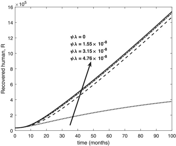
Variation of recovered human with re‐infection rates

FIGURE 4.

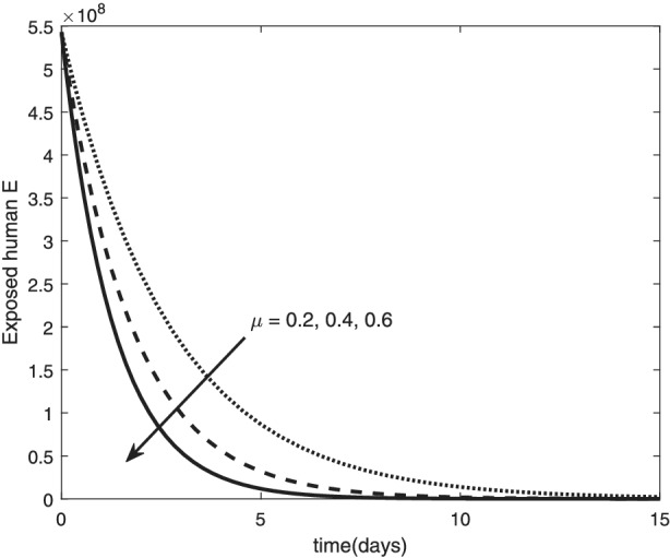
Variation of exposed human with death rate

The re‐infection rate measures the rate at which a recovered individual enters back into the infected population. As the re‐infection rate increases, more individuals enter into the exposed population, but a certain peak is quickly reached, and from that point onwards, the exposed population starts reducing (Figure 1). The implication is that the higher the re‐infection rate, the quicker the COVID‐19 transmission. As expected, both the asymptomatic and symptomatic infected population increase with increasing re‐infection rate (this is shown in Figure 2). By comparing Figure 2 with Figure 3, the recovered population is too low (barely 0.0001% of the infected population) compared with the infected population. This comparison shows the danger posed to the African population if recovered individual can be re‐infected with COVID‐19. Increase in the death rate μ invariably reduces the total population and consequently reduces the size of each compartment. This is depicted in Figures 4, 5, 6 below. With the current natural death rate in Africa standing below 0.15 and reducing yearly, it means that the infected population will continue to rise in Africa. Increasing case‐detection rate p helps to reveal the asymptomatic individuals more quickly for early treatment and thereby reduces the number of people who enter into the symptomatic population. This is depicted in Figure 7 where the asymptomatic infected population increases with increasing case‐detection rate, while symptomatic infected population decreases with increasing case‐detection rate. Increasing recovery rates r _a and r _s lead to a sharp reduction in the asymptomatic and symptomatic population as shown in Figure 8 while recovered population increases (see Figure 9).

FIGURE 1.

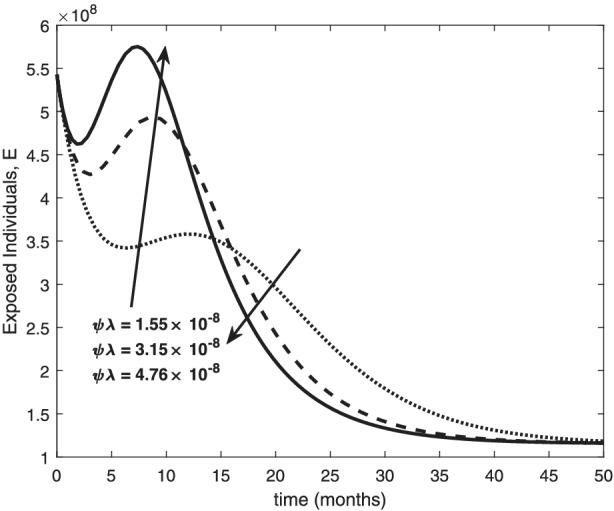
Variation of exposed human with recovery rates

FIGURE 2.

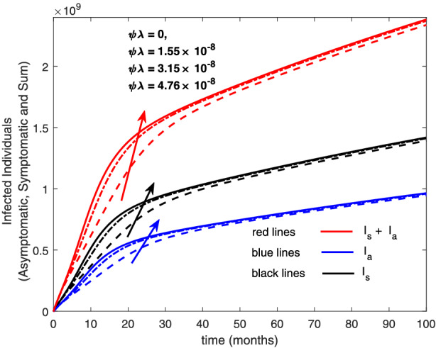
Variation of infected human with re‐infection rates [Colour figure can be viewed at wileyonlinelibrary.com]

FIGURE 5.

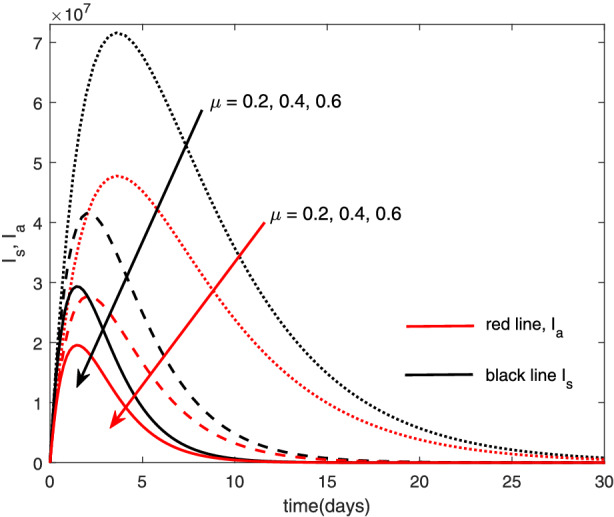
Variation of infected human with death rate [Colour figure can be viewed at wileyonlinelibrary.com]

FIGURE 6.

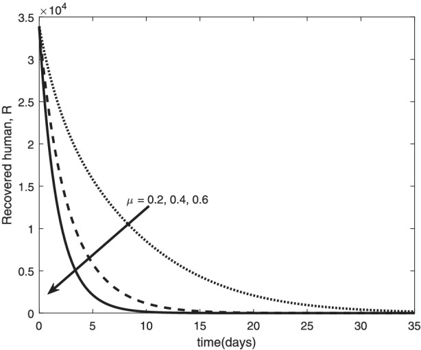
Variation of recovered human with death rate

FIGURE 7.

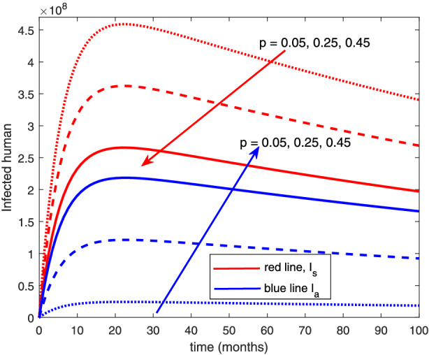
Variation of infected human with detection rate [Colour figure can be viewed at wileyonlinelibrary.com]

FIGURE 8.

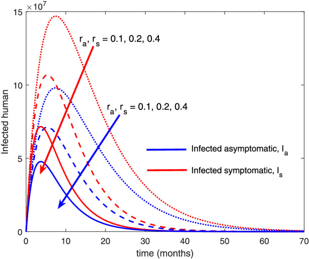
Variation of infected human with recovery rates [Colour figure can be viewed at wileyonlinelibrary.com]

FIGURE 9.

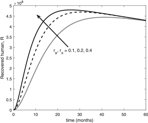
Variation of recovered human with recovery rates

5. DISCUSSION AND CONCLUSION

This study presents a mathematical model to study the spread of COVID‐19 in Africa. The model consists of a system of equations with the inclusion of asymptomatic case detection (p) and possible re‐infection of COVID‐19.

The analysis of this model is conducted by obtaining the reproduction number ℜ₀. Existence of backward bifurcation is tested and the local asymptotic stability of the DFE and the endemic equilibrium whenever the reproduction number ℜ₀ < 1 and ℜ₀ > 1, respectively, are established. The global asymptotic stability of the DFE and the endemic equilibrium for the model, without the re‐infection, is also established. The reproduction number is examined in respect to some parameters.

The results indicate that increasing case detection rate p will lead to a decrease in the symptomatic cases. Increasing case detection will reveal the true status of an individual and the asymptomatic individuals will call for early treatment, which in turn will reduce the number of asymptomatic individuals who migrate into the symptomatic population (this is why symptomatic population decreases with increasing case detection). Hence, repeated and increased testing to detect people living with the disease will be very effective in containing and reducing the burden of COVID‐19 in Africa.

As re‐infection rate increases, the exposed population is high for the first one and a half years until a large number of cases has been recorded in the African continent. More so, if re‐infection is possible, then the number of infected individuals will continue to rise without going down. In addition, since it has not been confirmed whether a recovered individual can be re‐infected, then enforcing a living condition where recovered individuals are not allowed to mix with the susceptible or exposed individuals will help in containing the spread of COVID‐19.

FUNDING INFORMATION

There are no funders to report for this submission.

CONFLICT OF INTEREST

This work does not have any conflicts of interest.

Oke AS, Bada OI, Rasaq G, Adodo V. Mathematical analysis of the dynamics of COVID‐19 in Africa under the influence of asymptomatic cases and re‐infection. Math Meth Appl Sci. 2022;45:137‐149. 10.1002/mma.7769

REFERENCES

- 1. Toit AD. Outbreak of a novel coronavirus. Nat Rev Microbiol. 2020;18(3):123‐123. [DOI] [PMC free article] [PubMed] [Google Scholar]
- 2. Oke AS. Convergence of differential transform method for ordinary differential equations. J Adv Math Comput Sci. 2017;24(6):1‐17. [Google Scholar]
- 3. Oke AS, Bada OI. Analysis of the dynamics of avian influenza A (H7N9) epidemic model with re‐infection. Open J Math Sci. 2019;3(1):417‐432. [Google Scholar]
- 4. Derwand R, Scholz M. Does zinc supplementation enhance the clinical efficacy of chloroquine/hydroxychloroquine to win today's battle against COVID‐19? Med Hypotheses. 2020;142:109815. [DOI] [PMC free article] [PubMed] [Google Scholar]
- 5. Hamizi K, Aouidane S, Belaaloui G. Etoposide‐based therapy for severe forms of COVID‐19. Med Hypotheses. 2020;142:109826. [DOI] [PMC free article] [PubMed] [Google Scholar]
- 6. Horowitz RI, Freeman PR. Three novel prevention, diagnostic, and treatment options for COVID‐19 urgently necessitating controlled randomized trials. Med Hypotheses. 2020;143:109851. [DOI] [PMC free article] [PubMed] [Google Scholar]
- 7. Hui DS, Azhar IE, Madani TA, Ntoumi F, Kock R, Dar O. The continuing 2019‐nCoV epidemic threat of novel coronaviruses to global health—the latest 2019 novel coronavirus outbreak in Wuhan, China. Int J Infect Dis. 2020;91:264‐266. [DOI] [PMC free article] [PubMed] [Google Scholar]
- 8. Kumar Raghav P, Mohanty S. Are graphene and graphene‐derived products capable of preventing COVID‐19 infection? Med Hypotheses. 2020;144:110031. [DOI] [PMC free article] [PubMed] [Google Scholar]
- 9. Salehi S, Abedi A, Balakrishnan S, Gholamrezanezhad A. Coronavirus disease 2019 (COVID‐19): a systematic review of imaging findings in 919 patients. AJR Am J Roentgenol. 2020;215(1):87‐93. [DOI] [PubMed] [Google Scholar]
- 10. Seifirad S. Pirfenidone: a novel hypothetical treatment for COVID‐19. Med Hypotheses. 2020;144:110005. [DOI] [PMC free article] [PubMed] [Google Scholar]
- 11. Taghizadeh‐Hesary F, Akbari H. The powerful immune system against powerful COVID‐19: A hypothesis. Med Hypotheses. 2020;140:109762. [DOI] [PMC free article] [PubMed] [Google Scholar]
- 12. Bada OI, Oke AS, Mutuku WN, Aye PO. Analysis of the dynamics of SI‐SI‐SEIR avian influenza A (H7N9) epidemic model with re‐infection. Earthline J Math Sci. 2021;5(1):43‐73. [Google Scholar]
- 13. Motta S, Pappalardo F. Mathematical modeling of biological systems. Brief Bioinform. 2012;14(4):411‐422. [DOI] [PubMed] [Google Scholar]
- 14. Tiwari M. A mathematical applications into the cells. J Nat Sci Biol Med. 2012;3(1):19‐23. [DOI] [PMC free article] [PubMed] [Google Scholar]
- 15. Aldila D, Khoshnaw SHA, Safitri E, et al. A mathematical study on the spread of COVID‐19 considering social distancing and rapid assessment: the case of Jakarta, Indonesia. Chaos Solitons Fract. 2020;110042. [DOI] [PMC free article] [PubMed] [Google Scholar]
- 16. Yang C, Wang J. A mathematical model for the novel coronavirus epidemic in Wuhan, China. Math Biosci Eng. 2020;17(3):2708‐2724. [DOI] [PMC free article] [PubMed] [Google Scholar]
- 17. Li Y, Wang B, Peng R, et al. Mathematical modeling and epidemic prediction of COVID‐19 and its significance to epidemic prevention and control measures. Ann Infect Dis Epidemiol. 2020. [Google Scholar]
- 18. Liang K. Mathematical model of infection kinetics and its analysis for COVID‐19, SARS and MERS. Infect Genet Evol. 2020;82:104306. [DOI] [PMC free article] [PubMed] [Google Scholar]
- 19. Wang N, Fu Y, Zhang H, Shi H. An evaluation of mathematical models for the outbreak of COVID‐19. Precision Clinical Medicine. 2020;3(2):85‐93. [DOI] [PMC free article] [PubMed] [Google Scholar]
- 20. Wang J. Mathematical models for COVID‐19: applications, limitations, and potentials. J Public Health Emergency. 2020;4:9. [DOI] [PMC free article] [PubMed] [Google Scholar]
- 21. Cooper I, Mondal A, Antonopoulos CG. A SIR model assumption for the spread of COVID‐19 in different communities. Chaos Solitons Fract. 2020;139:110057. [DOI] [PMC free article] [PubMed] [Google Scholar]
- 22. Annas S, Isbar Pratama M, Rifandi M, Sanusi W, Side S. Stability analysis and numerical simulation of SEIR Model for pandemic COVID‐19 spread in Indonesia. Chaos Solitons Fract. 2020;139:110072. [DOI] [PMC free article] [PubMed] [Google Scholar]
- 23. Riyapan P, Shuaib SE, Intarasit A. A mathematical model of COVID‐19 pandemic: a case study of Bangkok, Thailand. Comput Math Methods Med. 2021;2021(6664483):1‐11. [DOI] [PMC free article] [PubMed] [Google Scholar]
- 24. Ndairou F, Area I, Nieto JJ, Torres D. Mathematical modeling of COVID‐19 transmission dynamics with a case study of Wuhan. Chaos Solitons Fract, Advance Online Publication. 2020;135:109846. [DOI] [PMC free article] [PubMed] [Google Scholar]
- 25. Sarkar K, Khajanchi S, Nieto JJ. Modeling and forecasting the COVID‐19 pandemic in India. Chaos Solitons Fract. 2020;139:110049. [DOI] [PMC free article] [PubMed] [Google Scholar]
- 26. Okuonghae D, Omame A. Analysis of a mathematical model for COVID‐19 population dynamics in Lagos, Nigeria. Chaos Solitons Fract. 2020;139:110032. [DOI] [PMC free article] [PubMed] [Google Scholar]
- 27. Torrealba‐Rodriguez O, Conde‐Gutierrez RA, Hernandez‐Javier AL. Modeling and prediction of COVID‐19 in Mexico applying mathematical and computational models. Chaos Solitons Fract. 2020;138:109946. [DOI] [PMC free article] [PubMed] [Google Scholar]
- 28. Ivorra B, Ferrandez MR, Vela M, Ramos AM. Mathematical modeling of the spread of the coronavirus disease 2019 (COVID‐19) taking into account the undetected infections. The case of China. Commun Nonlin Sci Numer Simul. 2020;88:105303. [DOI] [PMC free article] [PubMed] [Google Scholar]
- 29. Wu J, Leung K, Leung GM. Nowcasting and forecasting the potential domestic and international spread of the 2019‐nCoV outbreak originating in Wuhan, China: a modelling study. Lancet. 2020;395(10225):689‐697. [DOI] [PMC free article] [PubMed] [Google Scholar]
- 30. Zhang Y, Yu X, Sun H, Tick GR, Wei W, Jin B. Applicability of time fractional derivative models for simulating the dynamics and mitigation scenarios of COVID‐19. Chaos Solitons Fract. 2020;138:109959. [DOI] [PMC free article] [PubMed] [Google Scholar]
- 31. James LP, Salomon JA, Buckee CO, Menzies NA. The use and misuse of mathematical modeling for infectious disease policymaking: lessons for the COVID‐19 pandemic. Med Decis Making. 2021;41(4):379‐385. [DOI] [PMC free article] [PubMed] [Google Scholar]
- 32. van den Driessche P, Watmough J. Reproduction numbers and sub‐threshold endemic equilibrium for compartment methods of the disease transmission. Math Biosci. 2002;180(1‐2):29‐48. [DOI] [PubMed] [Google Scholar]
- 33. Carr J. Applications of Centre Manifold Theory. New york: Springer; 1981. [Google Scholar]
- 34. Castillo‐Chavez C, Song B. Dynamical models of tuberculosis and their applications. Math Biosci Eng. 2004;1(2):361‐404. [DOI] [PubMed] [Google Scholar]
- 35. LaSalle JP, Lefschetz S. The Stability of Dynamical Systems. Philadelphia: SIAM; 1976. [Google Scholar]