A revisit to the past plague epidemic (India) versus the present COVID-19 pandemic: fractional-order chaotic models and fuzzy logic control

Abstract

India is one of the worst hit regions by the second wave of COVID-19 pandemic and ‘Black fungus’ epidemic. This paper revisits the Bombay Plague epidemic of India and presents six fractional-order models (FOMs) of the epidemic based on observational data. The models reveal chaotic dispersion and interactive coupling between multiple species of rodents. Suitable controllers based on fuzzy logic concept are designed to stabilise chaos to an infection-free equilibrium as well as to synchronise a chaotic trajectory with a regular non-chaotic one so that the unpredictability dies out. An FOM of COVID-19 is also proposed that displays chaotic propagation similar to the plague models. The index of memory and heredity that characterise FOMs are found to be crucial parameters in understanding the progression of the epidemics, capture the behaviour of transmission more accurately and reveal enriched complex dynamics of periodic to chaotic evolution, which otherwise remain unobserved in the integral models. The theoretical analyses successfully validated by numerical simulations signify that the results of the past Plague epidemic can be a pathway to identify infected regions with the closest scenarios for the present second wave of Covid-19, forecast the course of the outbreak, and adopt necessary control measures to eliminate chaotic transmission of the pandemic.

Introduction

Under the clutches of the second wave of COVID-19 pandemic, India is struggling to deal with the immediate crisis and emergency situation. The number of COVID-19-infected cases which was 18000 per day on 5th March, 2021, accelerated exponentially to 0.4 million in 2 months by 6th May in India, recording the highest ever total for a single day [1]. The unprecedented steep rate of propagation of the pandemic led to the over-burden of health infrastructure, saturation of medical facilities, shortage of vaccines, oxygen supply, hospital beds, etc., so much so that the number of deaths per day rose to a staggering 4454 by the end of May 2021. To worsen complications is the rising insurgent threat of another growing epidemic, ‘Black fungus’ or Mucormycosis, reported to have 9000 cases in India by May, 2021, particularly infecting post COVID victims with comorbidities such as Diabetes with a mortality rate of 50% [2]. Increase in testing measures and easing lockdown restrictions until March, 2021, were most likely the causes of the immediately following spikes in number of cases in the second wave of COVID in India by the month of April, 2021. These alarming figures signify the urgency of an efficient mathematical analysis and modelling of COVID-19 propagation so that its course of outbreak can be foreseen and controlled through a solution driven approach. This paper hereby proposes to study its complex dynamical evolution by revisiting a past epidemic that was the cause of numerous historically prominent pandemics: Plague.

The outbreak of Bombay (now Mumbai) Plague epidemic (1896–1911), India, was first reported in the British medical Journal, 1896 [3]. The surge in the casualties and infections dropped in 1897, but the epidemic turned into an endemic and lasted for more than a decade, returning every year with a seasonal dissemination. This has a close similarity with the COVID-19 pandemic, the first wave of which hit India in January 2020, and returned with a more severe second wave in early 2021, though it is too early to say whether it is seasonal. The bubonic plague, called so because of the development of buboes or sore lymph nodes in the infected, did not stay confined to Bombay alone, it hit all over India [4]. It is caused by bacillus Yersinia pestis and develops symptoms such as fever, vomiting, bleeding, organ failure, headache, weakness, etc. which if untreated may prove fatal in the first 36 hours of being infected [5]. Previous mathematical models of the plague epidemic are demonstrated by compartmental models based on the three compartments: susceptible, infected, recovered (SIR) [6] and fail to consider the transition of the disease between rodents and fleas. Plague is generally transmitted to humans by infected rodents who had been bitten by a flea. In fact, numerous species of rodents such as black rats, marmots, prairie dogs, gerbils, and squirrels are known carriers of plague [7]. Mathematical models of the epidemic based on nonlinear dynamics to study the interaction between a single species of rat and flea is proposed in 2012 by Bacaër et al. [8]. In 2015, a new model of plague was proposed in [5] that took into account multiple epizootics of rats such as Mus decumanus and Mus rattus. It led to the finding that the progression of the plague epidemic model displays chaotic behaviour. But all these models based on chaos theory are confined only to integer-order models (IOMs) which often fail to encompass in-depth understanding of the dynamics of the epidemic such as involvement of asymptomatic carriers, irregular transmission, critical cases with comorbidities, complexity of interaction amongst species, etc.

Fractional order models (FOMs), defined by fractional calculus, have an additional parameter of the non-integral derivative with an index of memory that incorporates various unmodelled dynamics of real physical systems resulting in a closer and more accurate interpretation of the model dynamics [9]. FOMs extract the underlying randomness in various engineering applications as switching circuits [10], jerk oscillators [11], hyperchaotic systems [12], homopolar disc dynamo [13], secure communication [14], etc. FOSs are known to produce various enriched complexities as period doubling route to chaos [15], oscillator dynamics [16], multistability [17], memristive dynamics [18], etc. In epidemiology, the memory and probability of transmission of FO chaotic models are found to be crucial parameters to capture the real dynamics of epidemic and infectious diseases [19]. For example, the FO-SIR chaotic compartmental model of Dengue epidemic is found to generate a closer fit to the observational data as validated from the Dengue cases of Malaysia [20]. The FO chaotic epidemic model of HIV comprising AIDS related cancer cells suggests that FOMs are better predictors and significantly impact the dynamic progress [21]. Also, nonlinear dynamic approach has been used to analyse cardiovascular diseases [22], a study especially relevant in the present COVID situation where heart patients are at greater risks of severe infections. Our work therefore, applies the superior benefits of fractional calculus and nonlinear dynamics approach to investigate the presence of chaos in the dispersal of plague epidemic and help in better understanding of the physiological functioning of infectious diseases.

Chaos, due to its high sensitivity to initial conditions, aperiodicity, erratic permanence and unpredictability, is an undesirable phenomenon in epidemiology [23]. This is why control of chaotic motion to stabilise it to a disease-free equilibrium or synchronise it with regular motion is a relevant area of research. Fuzzy logic control (FLC) has been a very practical and effective technique of controlling and synchronising chaos in nonlinear systems [24]. They are advantageous over conventional controllers since they are flexible over a wide range of operating conditions due to their soft logic principle and can be applicable to real-world systems with uncertainties and external disturbances, thus considerably reducing the tracking error and control effort [25]. The authors use the Takagi–Sugeno Fuzzy logic control (TS-FLC) [26] to suppress the undesirable effects of chaotic oscillations in the epidemic models.

The remainder of the paper is as follows: Section 2 presents the proposed FOMs of plague epidemic and relevant FO fundamentals, Sect. 3 depicts the design of controllers for stabilisation and synchronisation of the proposed models, and Sect. 4 presents the results and discussion. The paper is finally concluded in Sect. 5.

Fundamentals of FO calculus and proposed FO plague models (FOPMs)

The modelling of the epidemics and design of controllers to suppress chaos are determined by FO stability theorems whose preliminaries are presented below.

Preliminaries of FO

The Caputo fractional derivative, of order $\alpha$ of a continuous function f(t) is defined in (1).

$$\begin{array}{cc}\hfill D_t^{\alpha }f\left(t\right)=& \frac{{\text{d}}^{\alpha }f\left(t\right)}{{\text{d}t}^{\alpha }}\hfill \\ \hfill =& \left\{\begin{array}{cc}\frac{1}{\mathrm{\Gamma }\left(w,-\alpha \right)}\underset{0}{\overset{t}{\int }}\frac{f^{\left(w\right)}\left(\tau \right)}{{\left(t,-,\tau \right)}^{\alpha -w+1}}d\tau ,\hfill & w-1<\alpha <w,w\in N\hfill \\ \frac{d^w}{{\mathit{dt}}^w}f\left(t\right),\hfill & \alpha =w\hfill \end{array}\right)\hfill \\ \hfill \end{array}$$ 1

Let us define an FO nonlinear system (FONLS) as in (2),

$$\begin{array}{c}\hfill D_t^{\alpha }x\left(t\right)=f\left(x,\left(t\right),,,t\right),\end{array}$$ 2

where the FOs lie in $0<\alpha <1$ and $x(t)={[x_1,x_2,\dots ,x_n]}^T,(i=1,2,\dots ,n).$

Theorem 1

[27] Let $x=0$ be an equilibrium point for the FONLS (2), V(x) be a Lyapunov function, and ${\gamma }_i(i=1,2,3)$ be functions of class K such that

1. ${\gamma }_1(\Vert x\Vert )\le V(x)\le {\gamma }_2(\Vert x\Vert ),$

2. $D^{\alpha }V\left(x\right)\le -{\gamma }_3\left(\Vert ,x,\Vert \right)$,

where $\alpha \in (0,1)$, then, the equilibrium point $x=0$ is asymptotically stable.

For a quadratic positive definite function $V\left(x\right)=x^{T}Qx$, where Q is a positive definite matrix, the condition (a) of Theorem 1 is always satisfied [28].

Lemma 1

If $x(t)\in \mathfrak{R}$ is a continuous and derivable function, then, for any time instant $\ge 0$,

$$\begin{array}{c}\hfill \frac{1}{2}{D}^{\alpha }{x}^2\left(t\right)\le x\left(t\right)D^{\alpha }x\left(t\right),\forall \alpha \in (0,1],\end{array}$$

where $D^{\alpha }x\left(t\right)$ is the Caputo fractional derivative of $x\left(t\right)$ of FO $\alpha$.

The Adams–Bashforth–Moulton (ABM) method established on the predictor–corrector technique [29] is used to solve the FODEs.

FO plague models (FOPMs)

Recently, IOMs of chaotic plague epidemic models are proposed in [5] derived from the observational data on the number of deaths due to plague infection from September 1896 to December 1911 and coupling between the epidemic and the epizootic of the two main species of rodents using a global modelling technique. Based on this, we explore the FO dynamics of the models and propose six corresponding FOPMs where, $x_1,x_2$ and $x_3$ represent the number of fatalities due to plague infection, infected rats of the M. decumanus species captured and infected rats of the M. rattus species captured, respectively.

a) FOPM ${\mathit{P}}_{\mathbf{0}}$

$P_0$ is a 10-term chaotic model as in (3),

$$\begin{array}{c}\hfill \left\{\begin{array}{c}{D}^{\alpha }{x}_1=-0.0976x_3^2+0.045x_2{x}_3-12.6237\phi x_1\hfill \\ D^{\alpha }{x}_2=0.0107x_2^2-0.0237x_1{x}_2\hfill \\ D^{\alpha }{x}_3=0.0108x_3^2+1.4512x_2-5.912x_1\hfill \\ -0.0147x_1{x}_3+0.0041x_1{x}_2,\hfill \end{array}\right)\end{array}$$ 3

where tuning parameter $\phi =0.598$.

b) FOPM ${\mathit{P}}_{\mathbf{1}}$

$P_1$ is a 11-term chaotic model given as in (4), where $\phi =1$.

$$\begin{array}{c}\hfill \left\{\begin{array}{c}{D}^{\alpha }{x}_1=-0.0976x_3^2+0.045x_2{x}_3-12.6237\phi x_1\hfill \\ D^{\alpha }{x}_2=0.0107x_2^2-0.0237x_1{x}_2\hfill \\ D^{\alpha }{x}_3=0.0213x_3^2+2.0814x_2-6.917x_1\hfill \\ -0.0255x_1{x}_3+0.0078x_1{x}_2-0.0013x_2^2\hfill \end{array}\right)\end{array}$$ 4

c) FOPM ${\mathit{P}}_{\mathbf{2}}$

$P_2$ is also a 11-term chaotic model given as in (5), where $\phi =0.9.$

$$\begin{array}{c}\hfill \left\{\begin{array}{c}{D}^{\alpha }{x}_1=-0.1434x_3^2+0.0674x_2{x}_3\hfill \\ -12.7264\phi x_1-0.0025x_2^2\hfill \\ D^{\alpha }{x}_2=0.0107x_2^2-0.0237x_1{x}_2\hfill \\ D^{\alpha }{x}_3=0.0108x_3^2+1.4512x_2-5.912x_1\hfill \\ -0.0147x_1{x}_3+0.0041x_1{x}_2\hfill \end{array}\right)\end{array}$$ 5

d) FOPM ${\mathit{P}}_{\mathbf{3}}$

$P_3$ is a 12-term chaotic model given as in (6), where $\phi =0.945$.

$$\begin{array}{c}\hfill \left\{\begin{array}{c}{D}^{\alpha }{x}_1=-0.0936x_3^2+0.0431x_2{x}_3-12.0677\phi x_1\hfill \\ D^{\alpha }{x}_2=0.0103x_2^2-0.0227x_1{x}_2\hfill \\ D^{\alpha }{x}_3=0.0318x_3^2+1.7263x_2-6.6007x_1\hfill \\ -0.0355x_1{x}_3+0.005967x_1{x}_2\hfill \\ -0.004x_1^2-0.00007x_2^2\hfill \end{array}\right)\end{array}$$ 6

e) FOPM ${\mathit{P}}_{\mathbf{4}}$

$P_4$ is a 10-term periodic model given as in (7).

$$\begin{array}{c}\hfill \left\{\begin{array}{c}{D}^{\alpha }{x}_1=-0.0976x_3^2+0.045x_2{x}_3-12.6237{\phi x}_1\hfill \\ D^{\alpha }{x}_2=0.0107x_2^2-0.0237x_1{x}_2\hfill \\ D^{\alpha }{x}_3=0.0108x_3^2+1.4512x_2-5.912x_1\hfill \\ -0.0147x_1{x}_3+0.0041x_1{x}_2\hfill \end{array}\right)\end{array}$$ 7

This is the untuned $P_0$ model with, $\phi =1$.

f) FOPM ${\mathit{P}}_{\mathbf{5}}$

$P_5$ is a 11-term periodic model given as in (8).

$$\begin{array}{c}\hfill \left\{\begin{array}{c}{D}^{\alpha }{x}_1=-0.1434x_3^2+0.0674x_2{x}_3\hfill \\ -12.7264\phi x_1-0.0025x_2^2\hfill \\ D^{\alpha }{x}_2=0.0107x_2^2-0.0237x_1{x}_2\hfill \\ D^{\alpha }{x}_3=0.0108x_3^2+1.4512x_2-5.912x_1\hfill \\ -0.0147x_1{x}_3+0.0041x_1{x}_2\hfill \end{array}\right)\end{array}$$ 8

This is the untuned $P_2$ model with $\phi =1$.

Table 1 describes the initial conditions (ICs), equilibrium points, eigen values of the proposed FOPMs and their Lyapunov exponents (LEs) calculated using the algorithm proposed by Danca et al. [30].

Table 1.

Dynamical analyses of the FO plague epidemic models

Model	ICs	Equilibrium points	Eigen values $({\lambda }_i,i=1,2,3)$	FO	LEs	Dynamics
$P_0$	$\begin{array}{c}(166.8903,\hfill \\ 1070.193,\hfill \\ 138.7208)\hfill \end{array}$	$\begin{array}{c}{E}_1=(-2723.906,0,\hfill \\ -459.002)\hfill \end{array}$	${\lambda }_{1,2,3}=$ (64.556, − 9.44,32.0185)	0.98	$\begin{array}{c}\mathrm{L}{\mathrm{E}}_1=0.059548\hfill \\ \mathrm{L}{\mathrm{E}}_2=0\hfill \\ \mathrm{L}{\mathrm{E}}_3=-3.0896\hfill \end{array}$	Chaotic
		$E_2=(0,0,0)$	${\lambda }_{1,2,3}=$ (− 7.5489, 0,0)
		$E_3=$ $\begin{array}{c}(428.4239,948.939,\hfill \\ 97.436)\hfill \end{array}$	${\lambda }_{1,2,3}=$ $\begin{array}{c}(-7.2477,\hfill \\ 2.8296+11.2178i,\hfill \\ 2.8296-11.2178i)\hfill \end{array}$
$P_1$	$\begin{array}{c}(895.9957,\hfill \\ 2391.688,\hfill \\ 312.7087)\hfill \end{array}$	$E_1=(0,0,0)$	${\lambda }_{1,2,3}=$ (− 12.623, 0,0)	0.979	$\begin{array}{c}\mathrm{L}{\mathrm{E}}_1=0.22158\hfill \\ \mathrm{L}{\mathrm{E}}_2=0\hfill \\ \mathrm{L}{\mathrm{E}}_3=-0.45977\hfill \end{array}$	Chaotic
		$E_2=$ $\begin{array}{c}(-1112.367,0,\hfill \\ -379.308)\hfill \end{array}$	${\lambda }_{1,2,3}=$ (26.363, − 19.1324, 18.7156)
		$E_3=$ $\begin{array}{c}(533.355,1181.3568,\hfill \\ 200.333)\hfill \end{array}$	${\lambda }_{1,2,3}=$ $\begin{array}{c}(-7.8815,\hfill \\ 1.4159+12.3523i,\hfill \\ 1.4159-12.3523i)\hfill \end{array}$
$P_2$	$\begin{array}{c}(836.9658,\hfill \\ 1721.620,\hfill \\ 328.9299)\hfill \end{array}$	$E_1=(0,0,0)$	${\lambda }_{1,2,3}=$ (− 11.453,0,0)	0.996	$\begin{array}{c}\mathrm{L}{\mathrm{E}}_1=0.32517\hfill \\ \mathrm{L}{\mathrm{E}}_2=0\hfill \\ \mathrm{L}{\mathrm{E}}_3=-6.099\hfill \end{array}$	Chaotic
		$E_2=$ $\begin{array}{c}(-2659.1148,0,\hfill \\ -460.8589)\hfill \end{array}$	${\lambda }_{1,2,3}=$ (63.0210, − 14.0915, 31.7721)
		$E_3=$ $\begin{array}{c}(512.1487,1134.3856,\hfill \\ 178.6772)\hfill \end{array}$	${\lambda }_{1,2,3}=$ $\begin{array}{c}(-7.9728,\hfill \\ 2.4939+12.7008i,\hfill \\ 2.4939-12.7008i)\hfill \end{array}$
$P_3$	$\begin{array}{c}(344.0896,\hfill \\ 627.7882,\hfill \\ 101.5058)\hfill \end{array}$	$E_1=$ $\begin{array}{c}(810.5939,1786.4544,\hfill \\ 145.9542)\hfill \end{array}$	${\lambda }_{1,2,3}=$ $\begin{array}{c}(-17.624,\hfill \\ 2.5635+19.2493i,\hfill \\ 2.5635-19.2493i)\hfill \end{array}$	0.996	$\begin{array}{c}\mathrm{L}{\mathrm{E}}_1=0.76966\hfill \\ \mathrm{L}{\mathrm{E}}_2=0\hfill \\ \mathrm{L}{\mathrm{E}}_3=-15.0367\hfill \end{array}$	Chaotic
		$E_2=$ $\begin{array}{c}(1125.8296,2481.1972,\hfill \\ 1006.1933)\hfill \end{array}$	${\lambda }_{1,2,3}=$ $\begin{array}{c}(-6.9833+14.039i,\hfill \\ -6.9833-14.039i,\hfill \\ 52.146)\hfill \end{array}$
		$E_3=(0,0,0)$	${\lambda }_{1,2,3}=$ (- 11.403, 0, 0)
$P_4$	$\begin{array}{c}(166.8903,\hfill \\ 1070.193,\hfill \\ 138.7208)\hfill \end{array}$	$E_1=(0,0,0)$	${\lambda }_{1,2,3}=$ $\begin{array}{c}(-12.623,\hfill \\ 0,0)\hfill \end{array}$	0.938	$\begin{array}{c}\mathrm{L}{\mathrm{E}}_1=0\hfill \\ \mathrm{L}{\mathrm{E}}_2=-0.33791\hfill \\ \mathrm{L}{\mathrm{E}}_3=-6.4779\hfill \end{array}$	Periodic
		$E_2=$ $\begin{array}{c}(-1911.3082,0,\hfill \\ -497.203)\hfill \end{array}$	${\lambda }_{1,2,3}=$ $\begin{array}{c}(45.298,-16.6145,\hfill \\ 21.3474)\hfill \end{array}$
		$E_3=$ $\begin{array}{c}(532.1154,1178.6108,\hfill \\ 200.9904)\hfill \end{array}$	${\lambda }_{1,2,3}=$ $\begin{array}{c}(-6.1764,\hfill \\ 1.3416+12.8042i,\hfill \\ 1.3416-12.8042i)\hfill \end{array}$
$P_5$	$\begin{array}{c}(836.9658,\hfill \\ 1721.620,\hfill \\ 328.9299)\hfill \end{array}$	$E_1=(0,0,0)$	${\lambda }_{1,2,3}=$ (− 12.726, 0,0)	0.962	$\begin{array}{c}\mathrm{L}{\mathrm{E}}_1=0\hfill \\ \mathrm{L}{\mathrm{E}}_2=-0.059592\hfill \\ \mathrm{L}{\mathrm{E}}_3=-6.4876\hfill \end{array}$	Periodic
		$E_2=$ $\begin{array}{c}(534.5436,1183.9892,\hfill \\ 203.8006)\hfill \end{array}$	${\lambda }_{1,2,3}=$ $\begin{array}{c}(-7.4083,\hfill \\ 1.9474+13.0348i,\hfill \\ 1.9474-13.0348i)\hfill \end{array}$
		$E_3=$ $\begin{array}{c}(654.4082,1449.4837,\hfill \\ 486.6842)\hfill \end{array}$	${\lambda }_{1,2,3}=$ $\begin{array}{c}(4.9346,\hfill \\ -0.6295+19.7595i,\hfill \\ -0.6295-19.7595i)\hfill \end{array}$

Design of controllers for FOPMs

This section is dedicated to design controllers for two types of control: (a) stabilisation of chaos and (b) synchronisation of chaos.

Design of controllers for stabilisation of chaos in FOPMs

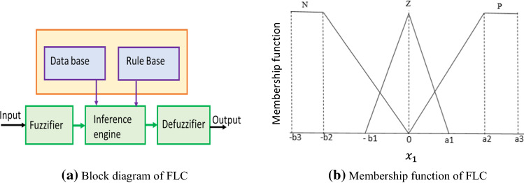
Stabilisation controllers to suppress chaos are applied only to the chaotic FOPMs, i.e., $P_0$, $P_1$, $P_2$ and $P_3$ as discussed in Table 1. As represented in Fig. 1a, TS Fuzzy Logic Control (TSFLC) [26] is designed with a rule base in which the consequents of each rule are functions of inputs, the fuzzifier converts the crisp inputs to linguistic variables using the membership functions stored in the database, the inference engine enables decision making by adequate reasoning and the defuzzifier converts the fuzzy output values back into crisp values.

Fig. 1.

Fuzzy Logic control system

Let the controlled FONLS be defined as in (9).

$$\begin{array}{c}\hfill D^{\alpha }x\left(t\right)=f\left(x,\left(t\right),,,t\right)+u\end{array}$$ 9

The control signal, $u={(u_1,u_2,\dots ,u_n)}^{\text{T}}$, is calculated by weighted sum defuzzification method.

The $i\text{th}$ fuzzy control rule base for the TSFLC is defined as in (10),

$$\begin{array}{cc}& \text{Rule}i:\text{IF}{x}_1\text{is}{X}_{i,1}\text{AND... AND}\hfill \\ \hfill & x_n\text{is}{X}_{i,n},\text{THEN}u=u_i\left(x\right),i=1,\dots ,r,r\in N^{\ast },\hfill \\ \hfill \end{array}$$ 10

where $X_{i,1},X_{i,2},\dots ,X_{i,n}$ are fuzzy sets describing the linguistic terms (LTs) of input variables, $u=u_i(x)$ is the control input of rule i, function AND is a fuzzy operator and r is the total number of fuzzy rules.

Each fuzzy rule defined in (10) generates a weight defined as in (11).

$$\begin{array}{c}\hfill {\omega }_i\in \left[0,,,1\right],i=1,2,\dots ,r\end{array}$$ 11

From (10), it is assumed that for any $x\in X$ in the input universe of discourse X, there exists at least one weight ${\omega }_i$ among all rules that is non-zero. Applying weighted sum defuzzification method, we obtain u as in (12).

$$\begin{array}{c}\hfill u=\frac{{\sum }_{i=1}^r{w}_i{u}_i}{{\sum }_{i=1}^r{w}_i}\end{array}$$ 12

Since a positive definite quadratic function always satisfies Theorem 1, the Lyapunov candidate is chosen as in (13).

$$\begin{array}{c}\hfill V\left(x\right)=x^{\text{T}}Qx.\end{array}$$ 13

$Q\in R^{\mathit{nxn}}$ is a positive definite matrix, which implies that V is positive definite, having continuous partial FO derivatives.

Theorem 2

[26] Let the origin be an equilibrium of the controlled epidemic (9) and there exists a Lyapunov function, $V\left(x\right)=x^{\text{T}}Qx$, where Q is a positive definite matrix on domain X containing the origin of $R^n$ such that $D^{\alpha }V\left(x\right)\le 0$, for $x\in X$. Let $S=\{x\in X:D^{\alpha }V\left(x\right)=0\}$. If except the trivial solution $x\left(t\right)\equiv 0$, no solution of (9) exists identically in S, then, the infection-free equilibrium at the origin is asymptotically stable in the domain X.

Using Theorem 2 based on FO Lyapunov stability, the stability of an infection free equilibrium may be obtained.

On adding TSFLC to the FOPM $P_1$ (4), we have (14),

$$\begin{array}{c}\hfill \left\{\begin{array}{c}{D}^{\alpha }{x}_1=-0.0976x_3^2+0.045x_2{x}_3-12.6237x_1+u_1\hfill \\ D^{\alpha }{x}_2=0.0107x_2^2-0.0237x_1{x}_2+u_2\hfill \\ D^{\alpha }{x}_3=0.0213x_3^2+2.0814x_2-6.917x_1\hfill \\ -0.0255x_1{x}_3+0.0078x_1{x}_2\hfill \\ -0.0013x_2^2+u_3\hfill \end{array}\right)\end{array}$$ 14

where $u={(u_1,u_2,u_3)}^T$ are the TSFLCs.

The fuzzification module of TSFLC in Fig. 1b) shows the triangular membership function of LTs of the chosen linguistic variable $x_1$ as antecedent. Notations P, Z and N for the LTs represent ‘positive’, ’zero’ and ‘negative’, respectively, and the parameters are chosen as $b3=500,b2=490,b1=10,a1=10,a2=1990,a3=2000.$

Table 2 describes the set of fuzzy control rules as per the membership function.

Table 2.

Rule base of TSFLCs for the chaotic FOPMs

Rule	Antecedent $x_1$	Consequent $u=\left[\begin{array}{c}{u}_1\\ u_2\\ u_3\end{array}\right]$
1	P	$U_1$
2	N	$U_2$
3	Z	$U_3$

The universe of discourse is $X=\left[-,500,,,2000\right]\times \left[0,,,3500\right]\times [-200,600].$

From (13), the Lyapunov function is chosen as (15).

$$\begin{array}{c}\hfill V\left(x\right)=\frac{1}{2}(x_1^2+x_2^2+x_3^2)\end{array}$$ 15

Using Lemma 1 and Caputo fractional derivative in (15), we have (16).

$$\begin{array}{cc}\hfill D^{\alpha }V\left(x\right)=& \frac{1}{2}{(D}^{\alpha }{x}_1^2+D^{\alpha }{x}_2^2+D^{\alpha }{x}_3^2)\hfill \\ \hfill \le & {(x}_1{D}^{\alpha }{x}_1+x_2{D}^{\alpha }{x}_2+x_3{D}^{\alpha }{x}_3).\hfill \end{array}$$ 16

From Theorem 1, we get

$$\begin{array}{cc}\hfill D^{\alpha }V\left(x\right)\le & x_1[-0.0976x_3^2+0.045x_2{x}_3\hfill \\ \hfill & -12.6237x_1+u_1]\hfill \\ \hfill & +x_2[0.0107x_2^2-0.0237x_1{x}_2+u_2]\hfill \\ \hfill & +x_3[0.0213x_3^2+2.0814x_2-6.917x_1\hfill \\ \hfill & -0.0255x_1{x}_3+0.0078x_1{x}_2\hfill \\ \hfill & -0.0013x_2^2+u_3].\hfill \end{array}$$ 17

Using Theorem 2, $D^{\alpha }V\left(x\right)=0\iff x={\left[0,,,0,,,0\right]}^T$ which implies $S=\{0,0,0\}$.

Next, the fuzzy rules are derived as follows.

• (i)Fuzzy rule 1, $R_1$: for antecedent $x_1$ as P, we have the consequent as

$$\begin{array}{c}\hfill U_1=\left[\begin{array}{c}{u}_1\hfill \\ u_2\hfill \\ u_3\hfill \end{array}\right]=\left[\begin{array}{c}0.1231x_3^2-0.0528x_2{x}_3+6.9174x_3\hfill \\ -0.0107x_2^2+0.0237x_1{x}_2-x_2-\frac{0.0213x_3^3}{x_2}-2.0814x_3\hfill \\ 0.0013x_2^2-x_3\hfill \end{array}\right],\end{array}$$

so that $D^{\alpha }V\left(x\right)\le -12.6237x_1^2-x_2^2-x_3^2<0$, i.e. the stability requirement is satisfied.

• (ii)Fuzzy rule 2, $R_2$: for antecedent $x_1$ as N, we have the consequent as

$$\begin{array}{cc}\hfill U_2=& \left[\begin{array}{c}{u}_1\hfill \\ u_2\hfill \\ u_3\hfill \end{array}\right]\hfill \\ \hfill =& \left[\begin{array}{c}0.1231x_3^2-0.0528x_2{x}_3+6.9174x_3\hfill \\ -0.0107x_2^2+0.0237x_1{x}_2-{4.77x}_2-\frac{0.0213x_3^3}{x_2}-2.0814x_3\hfill \\ 0.0013x_2^2-{2.12x}_3\hfill \end{array}\right],\hfill \end{array}$$

so that $D^{\alpha }V\left(x\right)\le =-12.6237x_1^2-4.77x_2^2-2.12x_3^2<0$, i.e. the stability requirement is satisfied.

• (iii)Fuzzy rule 3, $R_3$: for antecedent $x_1$ as Z, we have the consequent as

$$\begin{array}{c}\hfill U_3=\left[\begin{array}{c}{u}_1\hfill \\ u_2\hfill \\ u_3\hfill \end{array}\right]=\left[\begin{array}{c}0.1231x_3^2-0.0528x_2{x}_3+6.9174x_3\hfill \\ -0.0107x_2^2+0.0237x_1{x}_2-1.3164x_2-\frac{0.0213x_3^3}{x_2}-2.0814x_3\hfill \\ 0.0013x_2^2-6.247x_3\hfill \end{array}\right]\end{array}$$

so that $D^{\alpha }V\left(x\right)\le -12.6237x_1^2-1.3164x_2^2-6.247x_3^2<0$, i.e. the stability requirement is satisfied.

Since Theorem 2 is satisfied in the FO sense, thus the designed FLC converges the controlled epidemic $P_1$ to an infection-free asymptotically stable equilibrium. Similarly, the FLCs designed for the chaotic FOPMs $P_k$,$k=0,...,3$, and fuzzy rules, $R_i$ , where $i=1,2,3$ are enlisted in Table 3.

Table 3.

Proposed TSFLCs to stabilise chaos in FOPMs in antecedent ${\mathit{x}}_{\mathbf{1}}$

$P_k$	${\mathbf{R}}_{\mathbf{i}}$	Consequent	$P_k$	${\mathbf{R}}_{\mathbf{i}}$	Consequent
$P_0$	$R_1$	$U_1=\left[\begin{array}{c}{u}_1\\ u_2\\ u_3\end{array}\right]=\left[\begin{array}{c}0.1123x_3^2-0.0491x_2{x}_3+5.912x_3-\frac{x_3^2}{x_1}\\ -0.0107x_2^2+0.0237x_1{x}_2-x_2-\frac{0.0108x_3^3}{x_2}-1.4512x_3\\ 0\end{array}\right]$	$P_2$	$R_1$	$U_1=\left[\begin{array}{c}{u}_1\\ u_2\\ u_3\end{array}\right]$$=\left[\begin{array}{c}0.1581x_3^2-0.0688x_2{x}_3+5.912x_3\\ -0.0107x_2^2+0.0262x_1{x}_2-x_2-1.4512x_3-\frac{0.0108x_3^3}{x_2}\\ -0.0108x_3^2-x_3\end{array}\right]$
	$R_2$	$U_2=\left[\begin{array}{c}{u}_1\\ u_2\\ u_3\end{array}\right]=\left[\begin{array}{c}0.1123x_3^2-0.0491x_2{x}_3+5.912x_3-3.76\frac{x_3^2}{x_1}\\ -0.0107x_2^2+0.0237x_1{x}_2-2.93x_2-\frac{0.0108x_3^3}{x_2}-1.4512x_3\\ 0\end{array}\right]$		$R_2$	$U_2=\left[\begin{array}{c}{u}_1\\ u_2\\ u_3\end{array}\right]=\left[\begin{array}{c}0.1581x_3^2-0.0688x_2{x}_3+5.912x_3\\ -0.0107x_2^2+0.0262x_1{x}_2-3.92x_2-1.4512x_3-\frac{0.0108x_3^3}{x_2}\\ -0.0108x_3^2-1.4271x_3\end{array}\right]$
	$R_3$	$U_3=\left[\begin{array}{c}{u}_1\\ u_2\\ u_3\end{array}\right]=\left[\begin{array}{c}0.1123x_3^2-0.0491x_2{x}_3+5.912x_3-\frac{x_3^2}{x_1}\\ -0.0107x_2^2+0.0237x_1{x}_2-2.93x_2-\frac{0.0108x_3^3}{x_2}-1.4512x_3\\ -x_3\end{array}\right]$		$R_3$	$U_3=\left[\begin{array}{c}{u}_1\\ u_2\\ u_3\end{array}\right]=\left[\begin{array}{c}0.1581x_3^2-0.0688x_2{x}_3+5.912x_3\\ -0.0107x_2^2+0.0262x_1{x}_2-{5.98x}_2-1.4512x_3-\frac{0.0108x_3^3}{x_2}\\ -0.0108x_3^2-1.09374x_3\end{array}\right]$
$P_1$	$R_1$	$U_1=\left[\begin{array}{c}{u}_1\\ u_2\\ u_3\end{array}\right]=\left[\begin{array}{c}0.1231x_3^2-0.0528x_2{x}_3+6.9174x_3\\ -0.0107x_2^2+0.0237x_1{x}_2-x_2-\frac{0.0213x_3^3}{x_2}-2.0814x_3\\ 0.0013x_2^2-x_3\end{array}\right]$	$P_3$	$R_1$	$U_1=\left[\begin{array}{c}{u}_1\\ u_2\\ u_3\end{array}\right]=\left[\begin{array}{c}0.1291x_3^2-0.04906x_2{x}_3+0.004x_1{x}_3+6.007x_3\\ -0.0103x_2^2-1.7263x_3+0.0227x_1{x}_2+\left(0.00007\right)x_2{x}_3-x_2\\ -0.0318x_3^2-x_3\end{array}\right]$
	$R_2$	$U_2=\left[\begin{array}{c}{u}_1\\ u_2\\ u_3\end{array}\right]=$ $\left[\begin{array}{c}0.1231x_3^2-0.0528x_2{x}_3+6.9174x_3\\ -0.0107x_2^2+0.0237x_1{x}_2-{4.77x}_2-\frac{0.0213x_3^3}{x_2}-2.0814x_3\\ 0.0013x_2^2-{2.12x}_3\end{array}\right]$		$R_2$	$U_2=\left[\begin{array}{c}{u}_1\\ u_2\\ u_3\end{array}\right]=\left[\begin{array}{c}0.1291x_3^2-0.04906x_2{x}_3+0.004x_1{x}_3+6.007x_3\\ -0.0103x_2^2-1.7263x_3+0.0227x_1{x}_2+\left(0.00007\right)x_2{x}_3-4.57x_2\\ -0.0318x_3^2-1.75x_3\end{array}\right]$
	$R_3$	$U_3=\left[\begin{array}{c}{u}_1\\ u_2\\ u_3\end{array}\right]=$ $\left[\begin{array}{c}0.1231x_3^2-0.0528x_2{x}_3+6.9174x_3\\ -0.0107x_2^2+0.0237x_1{x}_2-1.3164x_2-\frac{0.0213x_3^3}{x_2}-2.0814x_3\\ 0.0013x_2^2-6.247x_3\end{array}\right]$		$R_3$	$U_3=\left[\begin{array}{c}{u}_1\\ u_2\\ u_3\end{array}\right]=\left[\begin{array}{c}0.1291x_3^2-0.04906x_2{x}_3+0.004x_1{x}_3+6.007x_3\\ -0.0103x_2^2-1.7263x_3+0.0227x_1{x}_2+\left(0.00007\right)x_2{x}_3-6.335x_2\\ -0.0318x_3^2-9.59x_3\end{array}\right]$

Design of TS-fuzzy logic synchronisation controllers (TSFLSCs) for synchronisation of chaos in FOPMs

The aim is to design a synchronisation controller u such that the dynamics of the slave system synchronises with the master system. Let the periodic and chaotic system as master and slave be defined in (18) and (19), respectively,

$$\begin{array}{c}\hfill D^{\alpha }y\left(t\right)=f\left(y,\left(t\right),,,t\right),\end{array}$$ 18

where $y(t)={[y_1,y_2,...,y_n]}^{\text{T}},(i=1,2,...,n)$ and

$$\begin{array}{c}\hfill D^{\alpha }x\left(t\right)=f\left(x,\left(t\right),,,t\right)+u_s,\end{array}$$ 19

where $x\left(t\right)={\left[x_1,,,,x_2,,,.,.,.,,,,x_n\right]}^{\text{T}};u_s={(u_{s1},u_{s2},...,u_{\mathit{sn}})}^{\text{T}}$ is the synchronisation controller added to synchronise the slave with the master.

The error states $e={\left[e_1,,,,e_2,,,.,.,.,,,e_n\right]}^{\text{T}}$ between the state variables of the master and slave systems are defined as in (20).

$$\begin{array}{c}\hfill e=x-y.\end{array}$$ 20

Thus, the FO error dynamics are obtained as in (21).

$$\begin{array}{c}\hfill D^{\alpha }e=D^{\alpha }x-D^{\alpha }y.\end{array}$$ 21

Therefore, the goal is to design $u_s$ such that e converge to zero as $t\to \infty ,$ i.e., the trajectory of the slave system asymptotically approaches the trajectory of the master system.

The $i^{\text{th}}$ fuzzy control rule for TSFLSC is defined as in (22),

$$\begin{array}{cc}& \text{Rule}i(R_i):\text{IF}{e}_1\text{is}{E}_{i,1}\text{AND... AND}{e}_n\text{is}\hfill \\ \hfill & E_{i,n},\text{THEN}{u}_{\mathit{si}}=u_i\left(e\right),i=1,\dots ,r,r\in N,\hfill \end{array}$$ 22

where $E_{i,1},E_{i,2},\dots ,E_{i,n}$ are fuzzy sets describing the LTs of input variables, $u_{\mathit{si}}=u_{\mathit{si}}(e)$ is the fuzzy logic synchronisation control input of $i^{\mathit{th}}$ rule following the same defuzzification process described in Sect. 3.1.

Each fuzzy rule defined in (22) generates a weight as in (23).

$$\begin{array}{c}\hfill {\partial }_i\in \left[0,,,1\right],i=1,...,r.\end{array}$$ 23

From (23), it is assumed that, for any $e\in E$ in the input universe of discourse E, there exists at least one weighted output among all rules that is non-zero. From the weighted sum of the defuzzification process, the output is as in (24),

$$\begin{array}{c}\hfill u_{\mathit{si}}=\frac{{\sum }_{i=1}^r{\partial }_i{u}_i}{{\sum }_{i=1}^r{\partial }_i},\end{array}$$ 24

where r is the total number of fuzzy rules.

A quadratic Lyapunov function is defined as in (25) which satisfies condition (a) of Theorem 1.

$$\begin{array}{c}\hfill V\left(e\right)=\frac{1}{2}(e_1^2+e_2^2+e_3^2+\cdots +e_n^2).\end{array}$$ 25

From Theorem 2, it can be concluded that, if the origin is an equilibrium of the controlled system (19) and $V\left(e\right)=\frac{1}{2}(e_1^2+e_2^2+e_3^2+\cdots +e_n^2)$ is a positive definite function on domain X containing the origin of $R^n$ such that $D^{\alpha }V\left(e\right)\le 0$, for $i=1,2,\dots ,r$ and $e\in E$, and $S=\{e\in E:D^{\alpha }V\left(e\right)=0\}$, and suppose no solution of (19) can stay identically in S except the trivial solution $e\left(t\right)\equiv 0$, then, the equilibrium at the origin is asymptotically stable in the domain E.

We now apply TSFLSC to synchronise the chaotic FOPM $P_0$ (3) as slave with the periodic $P_4$ as master, which is described in (26).

$$\begin{array}{c}\hfill \left\{\begin{array}{c}{D}^{\alpha }{y}_1=-0.0976y_3^2+0.045y_2{y}_3-12.6237y_1\hfill \\ D^{\alpha }{y}_2=0.0107y_2^2-0.0237y_1{y}_2\hfill \\ D^{\alpha }{y}_3=0.0108y_3^2+1.4512y_2-5.912y_1\hfill \\ -0.0147y_1{y}_3+0.0041y_1{y}_2\hfill \end{array}\right)\end{array}$$ 26

From (21), the error dynamics are given by (27).

$$\begin{array}{c}\hfill \left\{\begin{array}{c}{D^{\alpha }e}_1=-0.0976{(x}_3^2-y_3^2)+0.045(x_2{x}_3-y_2{y}_3)\hfill \\ -7.5489726x_1+12.6237y_1+u_{s1}\hfill \\ {D^{\alpha }e}_2=0.0107{(x}_2^2-y_2^2)\hfill \\ -0.0237(x_1{x}_2-y_1{y}_2)+u_{s2}\hfill \\ {D^{\alpha }e}_3=0.0108\left(x_3^2,-,y_3^2\right)+1.4512e_2-5.912e_1\hfill \\ -0.0147{(x}_1{x}_3-y_1{y}_3)\hfill \\ +0.0041(x_1{x}_2-y_1{y}_2)+u_{s3}\hfill \end{array},.\right)\end{array}$$ 27

The parameters of Fig. 1b chosen are $b3=1500,b2=1480,b1=20,a1=20,a2=1480,a3=1500$ so that $E=\left[-,1500,,,1500\right]\times \left[-,2500,,,2000\right]\times [-800,600]$.

From (25), the Lyapunov function is chosen as in (28).

$$\begin{array}{c}\hfill V\left(e\right)=\frac{1}{2}(e_1^2+e_2^2+e_3^2).\end{array}$$ 28

Using Caputo derivative in (28), we have (29).

$$\begin{array}{c}\hfill D^{\alpha }V\left(e\right)=\frac{1}{2}{(D}^{\alpha }{e}_1^2+D^{\alpha }{e}_2^2+D^{\alpha }{e}_3^2).\end{array}$$ 29

The fuzzy rules are derived as follows.

• (i)Fuzzy rule 1, $R_1$: for antecedent $e_1$ as P, we have the consequent as

$$\begin{array}{cc}\hfill U_1=& \left[\begin{array}{c}{u}_{s1}\hfill \\ u_{s2}\hfill \\ u_{s3}\hfill \end{array}\right]=\left[\begin{array}{c}0.0976{(x}_3^2-y_3^2)-0.045(x_2{x}_3-y_2{y}_3)+7.5489726x_1-12.6237y_1-e_1+5.912e_3\hfill \\ -0.0107{(x}_2^2-y_2^2)+0.0237(x_1{x}_2-y_1{y}_2)-e_2-1.4512e_3\hfill \\ -0.0108\left(x_3^2,-,y_3^2\right)+0.0147{(x}_1{x}_3-y_1{y}_3)-0.0041(x_1{x}_2-y_1{y}_2)-e_3\hfill \end{array}\right],\hfill \end{array}$$

then from (29), $D^{\alpha }V(e)=-e_1^2-e_2^2-e_3^2<0.$

• (ii)Fuzzy rule 2, $R_2$: for antecedent $e_1$ as N, we have the consequent as

$$\begin{array}{cc}& U_2=\left[\begin{array}{c}{u}_{s1}\hfill \\ u_{s2}\hfill \\ u_{s3}\hfill \end{array}\right]=\left[\begin{array}{c}0.0976{(x}_3^2-y_3^2)-0.045(x_2{x}_3-y_2{y}_3)+7.5489726x_1-12.6237y_1-6.5e_1+5.912e_3\hfill \\ -0.0107{(x}_2^2-y_2^2)+0.0237(x_1{x}_2-y_1{y}_2)-9.5e_2-1.4512e_3\hfill \\ -0.0108\left(x_3^2,-,y_3^2\right)+0.0147{(x}_1{x}_3-y_1{y}_3)-0.0041(x_1{x}_2-y_1{y}_2)-e_3\hfill \end{array}\right].\hfill \end{array}$$

Then from (29), $D^{\alpha }V(e)=-6.5e_1^2-9.5e_2^2-e_3^2<0$.

• (iii)Fuzzy rule 3, $R_3$: for antecedent $e_1$ as Z, we have the consequent as

$$\begin{array}{cc}& U_3=\left[\begin{array}{c}{u}_{s1}\hfill \\ u_{s2}\hfill \\ u_{s3}\hfill \end{array}\right]=\left[\begin{array}{c}0.0976{(x}_3^2-y_3^2)-0.045(x_2{x}_3-y_2{y}_3)+7.5489726x_1-12.6237y_1-6.5e_1+5.912e_3\hfill \\ -0.0107{(x}_2^2-y_2^2)+0.0237(x_1{x}_2-y_1{y}_2)-9.5e_2-1.4512e_3\hfill \\ -0.0108\left(x_3^2,-,y_3^2\right)+0.0147{(x}_1{x}_3-y_1{y}_3)-0.0041(x_1{x}_2-y_1{y}_2)-13e_3\hfill \end{array}\right].\hfill \end{array}$$

Then from (29),$D^{\alpha }V(e)=-6.5e_1^2-9.5e_2^2-13e_3^2<0$.

Since $D^{\alpha }V(e)=0\iff e={\left[0,,,0,,,0\right]}^T$ which implies $S=\{0,0,0\}$. Thus, the errors, $e={[e_1,e_2,e_3]}^T$ converge to zero and the slave $P_0$ synchronises with the master $P_4$. Similarly, the TSFLSC designed to synchronise FOPMs, the chaotic $P_2$ with the periodic $P_5$ is as in Table 4.

Table 4.

Proposed TSFLSC for synchronisation in FOPMs, ${\mathit{P}}_{\mathbf{0}}$ (slave) with ${\mathit{P}}_{\mathbf{4}}$ (master); and ${\mathit{P}}_{\mathbf{2}}$ (slave) with ${\mathit{P}}_{\mathbf{5}}$ (master) at antecedent ${\mathit{e}}_{\mathbf{1}}$

Master system	Slave system	Rule $\mathit{i}$	Consequent synchronisation controller
$P_4$	$P_0$	$R_1$	$U_1=\left[\begin{array}{c}0.0976{(x}_3^2-y_3^2)-0.045(x_2{x}_3-y_2{y}_3)+7.5489726x_1-12.6237y_1-e_1+5.912e_3\hfill \\ -0.0107{(x}_2^2-y_2^2)+0.0237(x_1{x}_2-y_1{y}_2)-e_2-1.4512e_3\hfill \\ -0.0108\left(x_3^2,-,y_3^2\right)+0.0147{(x}_1{x}_3-y_1{y}_3)-0.0041(x_1{x}_2-y_1{y}_2)-e_3\hfill \end{array}\right]$
		$R_2$	$U_2=\left[\begin{array}{c}0.0976{(x}_3^2-y_3^2)-0.045(x_2{x}_3-y_2{y}_3)+7.5489726x_1-12.6237y_1-6.5e_1+5.912e_3\hfill \\ -0.0107{(x}_2^2-y_2^2)+0.0237(x_1{x}_2-y_1{y}_2)-9.5e_2-1.4512e_3\hfill \\ -0.0108\left(x_3^2,-,y_3^2\right)+0.0147{(x}_1{x}_3-y_1{y}_3)-0.0041(x_1{x}_2-y_1{y}_2)-e_3\hfill \end{array}\right]$
		$R_3$	$U_3=\left[\begin{array}{c}0.0976{(x}_3^2-y_3^2)-0.045(x_2{x}_3-y_2{y}_3)+7.5489726x_1-12.6237y_1-6.5e_1+5.912e_3\hfill \\ -0.0107{(x}_2^2-y_2^2)+0.0237(x_1{x}_2-y_1{y}_2)-9.5e_2-1.4512e_3\hfill \\ -0.0108\left(x_3^2,-,y_3^2\right)+0.0147{(x}_1{x}_3-y_1{y}_3)-0.0041(x_1{x}_2-y_1{y}_2)-13e_3\hfill \end{array}\right]$
$P_5$	$P_2$	$R_1$	$U_1=\left[\begin{array}{c}0.1434{(x}_3^2-y_3^2)-0.0674(x_2{x}_3-y_2{y}_3)+0.0025{(x}_2^2-y_2^2)+11.45376x_1-12.7264y_1-e_1+5.912e_3\hfill \\ -0.0107{(x}_2^2-y_2^2)+0.0237(x_1{x}_2-y_1{y}_2)-e_2-1.4512e_3\hfill \\ -0.0108\left(x_3^2,-,y_3^2\right)+0.0147{(x}_1{x}_3-y_1{y}_3)-0.0041(x_1{x}_2-y_1{y}_2)-e_3\hfill \end{array}\right]$
		$R_2$	$U_2=\left[\begin{array}{c}{0.1434(x}_3^2-y_3^2)-0.0674(x_2{x}_3-y_2{y}_3)+0.0025{(x}_2^2-y_2^2)+11.45376x_1-12.7264y_1-7.5e_1+5.912e_3\hfill \\ -0.0107{(x}_2^2-y_2^2)+0.0237(x_1{x}_2-y_1{y}_2)-10.5e_2-1.4512e_3\hfill \\ -0.0108\left(x_3^2,-,y_3^2\right)+0.0147{(x}_1{x}_3-y_1{y}_3)-0.0041(x_1{x}_2-y_1{y}_2)-e_3\hfill \end{array}\right]$
		$R_3$	$U_3=\left[\begin{array}{c}{0.1434(x}_3^2-y_3^2)-0.0674(x_2{x}_3-y_2{y}_3)+0.0025{(x}_2^2-y_2^2)+11.45376x_1-12.7264y_1-7.5e_1+5.912e_3\hfill \\ -0.0107{(x}_2^2-y_2^2)+0.0237(x_1{x}_2-y_1{y}_2)-10.5e_2-1.4512e_3\hfill \\ -0.0108\left(x_3^2,-,y_3^2\right)+0.0147{(x}_1{x}_3-y_1{y}_3)-0.0041(x_1{x}_2-y_1{y}_2)-15e_3\hfill \end{array}\right]$

Results and discussion

Results obtained from numerical simulation are discussed in the following subsections.

Dynamical analyses of FOPM

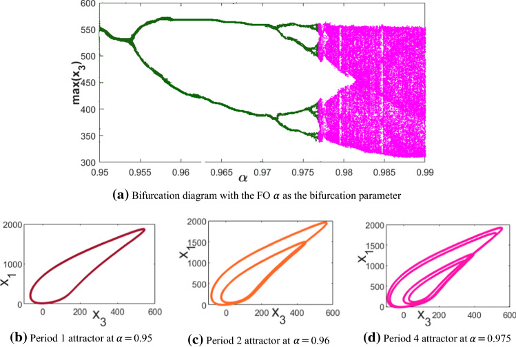
The bifurcation analysis of FOPM $P_1$ (4) is performed in Fig. 2a for a varying FO $\alpha$ as the bifurcation parameter against $x_3$ that represents the number of captured infected rats of M. rattus species. It is revealed that plague follows a path of multiple period doublings to finally give rise to chaos at $\alpha =0.977$. The Period 1 attractor (P1A) that persists in the region $\alpha \in [0.95,954[$ is shown in Fig. 2b. P1A doubles its period to a Period 2 attractor (P2A) that persists in the region $\alpha \in [0.954,0.972[$ and is displayed in Fig. 2c. Similarly, a Period 4 attractor (P4A) existing in the range $\alpha \in [0.972,0.9755[$ is illustrated in Fig. 2d and the final chaotic attractor from $\alpha =0.977$ onwards in Fig. 3b.

Fig. 2.

Attractors and bifurcation of period doubling route to chaos in FO plague model $P_1$

Fig. 3.

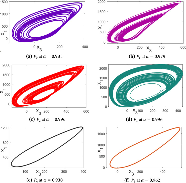
Attractors of proposed FO plague models

Figure 3 depicts the dynamics of attractors of the FOPMs as investigated in Table 1 of Sect. 2.2.

It is observed that $P_0,P_1,P_2,P_3$ display chaotic dynamics and $P_4,P_5$ display periodic dynamics.

Stabilisation of chaos in FOPMs using TSFLC

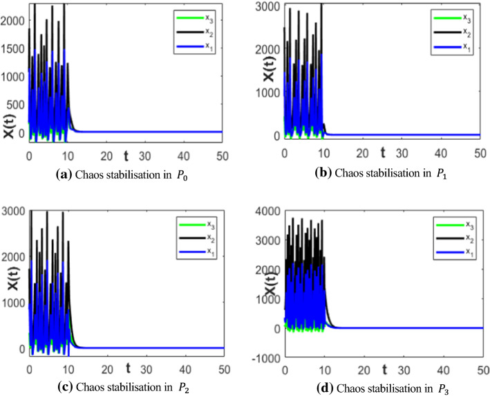
Since, only the FOPMs, $P_0,P_1,P_2,P_3$ display chaotic dynamics, hence the controllers designed using TSFLC concept in Sect. 3.1 are added to the corresponding plague models at 10 s. It is observed from the plots of Fig. 4 that chaos dies out within 4 s once the controller is applied.

Fig. 4.

Stabilisation of chaos in FO plague epidemic models when controller is added at 10 s

Synchronisation of chaos in FOPM using TSFLSC

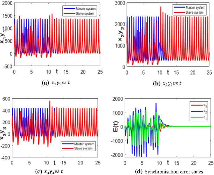
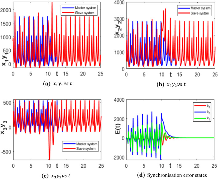
Another way of suppressing chaotic dynamics in plague epidemic model is using synchronisation controller. The significance lies in the fact that the uncontrolled chaotic dynamics of the slave epidemic model after controlled synchronisation becomes asymptotically periodic which means that the motion of its trajectories repeats after fixed intervals of time with a constant period and is imperturbable to minute changes in initial states of physical parameters. In real situations, such definite repetitive dynamics makes prediction of the epidemic model easier. The numerical results of synchronisation controllers designed in Sect. 3.2 are plotted in Figs. 5 and 6, where it is clear that on adding the TSFLSCs at 10 s, the initially chaotic slaves $P_0$ and $P_2$ display periodic dynamics once they are synchronised with the masters $P_4$ and $P_5$, respectively.

Fig. 5.

Synchronisation control between $P_4$(master) and $P_0$(slave) plague epidemic models using TSFLSC

Fig. 6.

Synchronisation control between $P_5$(master) and $P_2$(slave) plague epidemic models using TSFLSC

Comparative analyses between the plague epidemic and COVID-19 pandemic models

The IOM of chaotic COVID-19 pandemic is modelled using global modelling technique [31] obtained from two real data sets: the official data from the National Health Commission of the People’s Republic of China [32] and the data from the Johns Hopkins University [33]. The FO COVID-19 model (FOCM) is proposed in (30),

$$\begin{array}{c}\hfill \left\{\begin{array}{c}{D}^{\alpha }{x}_1=-0.10530723x_3^2+2.343\times {10}^{-5}{x}_1^2\hfill \\ -0.15204x_2(x_3-0.01451520x_1)\hfill \\ D^{\alpha }{x}_2=-0.20517824x_1+0.44040714x_2\hfill \\ +0.16060376x_3^2\hfill \\ D^{\alpha }{x}_3=-0.00011493x_1{x}_3-1.215\times {10}^{-5}{x}_1{x}_2\hfill \\ +0.2844499x_3+2.38\times {10}^{-6}{x}_1{x}_2\hfill \end{array}\right)\end{array}$$ 30

where $x_1,x_2,x_3$ are the numbers of confirmed cases, critical cases under intensive care and cumulative number of fatalities per day, respectively.

In terms of dynamical analysis, it is observed that the FOCM (30) undergoes period doubling bifurcation to generate chaotic transmission with the gradual increase in FO; similar to that of the plague model. The bifurcation diagram plotted in Fig. 7 for the trajectory corresponding to cumulative number of COVID-19 infected deaths per day, reveals that it follows a rich complex dynamical path through successive cascades of period doubling which otherwise remain unobserved in the IO chaotic model. The FOCM displays a P1A in $\alpha ϵ[0.95,0.96]$, which gets converted to a P2A in [0.96, 0.97]. It splits further to transform into a P4A that gives birth to chaotic attractor after infinite doublings from $\alpha =0.974$ onwards.

Fig. 7.

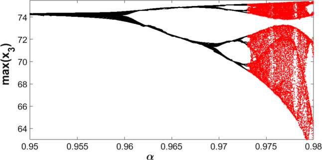
Period doubling bifurcation of FO COVID-19 pandemic model

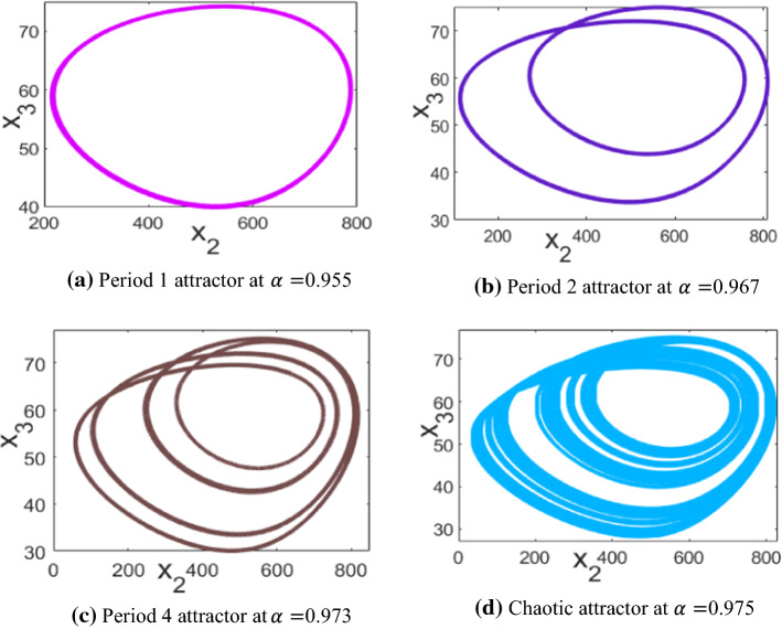
The corresponding attractors of FOCM are plotted in Fig. 8 that shows asymptotically period doubling route to chaos.

Fig. 8.

Phase portraits of FO COVID-19 pandemic model

The above results and analyses lead to the following qualitative comparisons between the plague epidemic and the COVID-19 pandemic situation in India:

• (i)Both plague and COVID-19 propagation dynamics are governed by chaotic behaviour where an apparently trivial event may trigger a series of divergent events, indicating that a long-term prediction of the spread of the epidemic is not possible. One of the major shortcomings of recent mathematical models to exactly predict the course of COVID-19 is that they do not take into account the chaotic behaviour of the spread [34].
• (ii)COVID-19 is a multi-strain pandemic, a characteristic similar to plague. More than 100 strains of COVID-19 have been discovered as reported in Brazil [35], the United Kingdom [36], South Africa [37], etc. The Covid-19 virus has undergone multiple mutations of which the variants named as ‘Kappa’ and ‘Delta’ by WHO [38], first discovered in India, in October, 2020 are far more contagious than their predecessors having a transmission rate of 2.5 times faster.
• (iii)The plague epidemic sustained repeated seasonal waves lasting for over 15 years (1896–1911), while the ongoing COVID-19 pandemic too has repeated waves of resurgence pointing towards the possibility of a third wave in India [39].
• (iv)Both plague and COVID-19 dispersal in India have displayed close similarities demographically as well as geographically. The Bombay Plague first hit Mumbai in 1896 and then spread all over India [5]. Similarly, Mumbai was one of the first and worst hit cities in India in both the first and second waves of Covid-19 which gradually disseminated with a rapid transmission rate throughout the country.

The control framework in real scenario may reflect cost effective treatments, social mobility restrictions, injection of vaccines and prophylactic drugs, delays, effective planning on medical infrastructure as hospital beds, ventilators, oxygen cylinders, ICU berths, ambulance, etc. and providing other health facilities. In our future scope of work, we shall explore the design of the controllers based on these actual control measures. Sensing and control strategies can be applied for close monitoring of the epidemic activities using real time technology such as remote sensors, web-based tools for surveillance, tracking individual movements, e- government initiatives such as the Aarogya Setu [40], high throughput sequencing technology, etc. [41]. In fact, lower-middle income countries like India need judicious planning on executing control policies to evaluate the risk and cost of prophylactic strategies and public health policies depending on the short-term estimation of the chaotic course of the pandemic based on past experience.

Conclusions

This paper investigates the complex dynamics of fractional-order models of the past plague epidemic which hit India over a hundred years ago and lasted for more than a decade. We also analyse the FOM of COVID-19 pandemic and found that both epidemics are multi-strain models, have probable seasonality, drastic transmission rate in high population density areas of India, manifest chaotic wave of propagation, all striking close similarities demographically and geographically. Both plague and COVID-19 are found to exhibit chaotic behaviour, which means a small change in a trivial event may activate a series of divergent unpredictable events due to their hyped sensitivity to initial states of driving parameters. Two types of controllers are proposed to suppress chaos in the epidemic: first, stabilisation control, where a TS fuzzy logic controller is designed that successfully stabilises the chaotic dynamics of the epidemic by minimizing the numbers of infections, critical cases and fatalities to a disease-free equilibrium, and second, synchronisation control, where the proposed controller efficiently synchronises the chaotic dynamics of the slave with the regular periodic dynamics of the master. It is significant since after synchronisation, the originally chaotic slave epidemic model transforms into a periodic one which means that its flow repeats after fixed intervals of time with a constant period and is no longer sensitive to small perturbations of parameters. In real situations, such repeated regular dynamics facilitates prediction of the course of outbreak, since the next surge or spike in infections occurring at a periodic regular interval can be estimated beforehand and an early alarm can be set. The proposed FOMs, possessing the features of flexibility, heredity and memory, can provide more accurate models of the chaotic pandemics by incorporating unmodelled dynamics that often fail to be encompassed by integer-order models. It was discovered that in both plague and COVID-19 models, with stronger index of memory (lower values of fractional-order), chaos subsides into regular periodic dynamics, while as memory weakens and fades away towards an integral order, the route to chaos in transmission dynamics is evident. In our future scope of work, we shall explore the design of the controllers based on real control measures Thus, the authors are hopeful that the results on the chaotic dynamics of propagation of the epidemic will be helpful to recognise regions with high risk of contamination and initiate timely action on crisis assessment, hazard management, policy making, emergency planning and economic control measures, i.e. learning from the knowledge of the past.

Data Availability Statement

This manuscript has associated data in a data repository. [Author comments’: Interested readers may contact the authors for details.]

References

- 1.COVID-19 Data Repository by the Center for Systems Science and Engineering (CSSE) at Johns Hopkins University, https://github.com/CSSEGISandData/COVID-19
- 2.Indian Council of Medical Research (ICMR) (2021). https://www.icmr.gov.in/pdf/covid/techdoc/Mucormycosis_ADVISORY_FROM_ICMR_In_COVID19_time.pdf
- 3.The reported appearance of plague in Bombay. Br. Med. J. 1886, 966 (1896) [PMC free article] [PubMed]
- 4.Pollitzer R. Plague. Geneva: WHO; 1954. p. 409. [Google Scholar]
- 5.Mangiarotti S. Chaos Solitons Fractals. 2015;81:184. doi: 10.1016/j.chaos.2015.09.014. [DOI] [Google Scholar]
- 6.Raggett GF. Inst. Math. Appl. 1982;18:221. [Google Scholar]
- 7.Plague Research Commission The epidemiological observations made by the commissioning Bombay city. J. Hyg. 1907;7:724. doi: 10.1017/s0022172400033684. [DOI] [PMC free article] [PubMed] [Google Scholar]
- 8.Bacaër N. J. Math. Biol. 2012;64:403. doi: 10.1007/s00285-011-0417-5. [DOI] [PubMed] [Google Scholar]
- 9.Zhou P, Ma J, Tang J. Nonlinear Dyn. 2020;100:2353. doi: 10.1007/s11071-020-05637-z. [DOI] [Google Scholar]
- 10.M. Borah, B. K. Roy, Switching synchronisation control between integer-order and fractional-order dynamics of a chaotic system. In: IEEE Indian Control Conference, IIT Guwahati, India, pp. 456–461 (2017)
- 11.Rajagopal K, Akgul A, Jafari S, Karthikeyan A, Cavusoglu U, Kacar S. Soft Comput. 2020;1:7469–7479. doi: 10.1007/s00500-019-04373-w. [DOI] [Google Scholar]
- 12.Borah M, Roy BK. Chaos Solitons Fractals. 2020;131:109539. doi: 10.1016/j.chaos.2019.109539. [DOI] [Google Scholar]
- 13.Z Wei, Y Li, K Rajagopal, Mechatron. Syst. Control, (2020). 10.2316/j.2020.201-0034
- 14.M. Borah, B. K. Roy, A novel multi-wing fractional-order chaotic system, its synchronisation control and application in secure communication. In: IEEE International Conference on Energy, Power and Environment (ICEPE), NIT Meghalaya, India, pp. 1–6. (2018) 10.1140/epjst/e2018-00063-9
- 15.Borah M, Roy BK. Eur. Phys. J. Spec. Top. 2017;226:3747. doi: 10.1140/epjst/e2018-00063-9. [DOI] [PMC free article] [PubMed] [Google Scholar]
- 16.Akgul A. J. Circuits Syst. Comput. 2019;28:1950239. doi: 10.1142/S0218126619502396. [DOI] [Google Scholar]
- 17.Borah M. J. Comput. Nonlinear Dyn. 2018;13:090906. doi: 10.1115/1.4039841. [DOI] [Google Scholar]
- 18.Borah M, Roy BK. Eur. Phys. J. Spec. Top. 2021 doi: 10.1140/epjs/s11734-021-00179-w. [DOI] [PMC free article] [PubMed] [Google Scholar]
- 19.Qureshi S, Jan R. Chaos Solitons Fractals. 2021;145:110766. doi: 10.1016/j.chaos.2021.110766. [DOI] [PMC free article] [PubMed] [Google Scholar]
- 20.Hamdan NI, Kilicman A. Chaos Solitons Fractals. 2018;114:55. doi: 10.1016/j.chaos.2018.06.031. [DOI] [Google Scholar]
- 21.Naik PA, Owolabi KM, Yavuz M, Zu J. Chaos Solitons Fractals. 2020;140:110272. doi: 10.1016/j.chaos.2020.110272. [DOI] [PMC free article] [PubMed] [Google Scholar]
- 22.Cheffer A, Savi MA, Pereira TL, de Paula AS. Appl. Math. Model. 2021;96:152. doi: 10.1016/j.apm.2021.03.014. [DOI] [Google Scholar]
- 23.J. Duarte, C. Januário, N. Martins, J. Seoane, M.A.F. Sanjuán, arXiv preprint arXiv:2102.08284, (2021)
- 24.Nazarimehr F, Sheikh J, Ahmadi MM, Pham VT, Jafari S. Chaos Solitons Fractals. 2018;106:349. doi: 10.1016/j.chaos.2017.12.005. [DOI] [Google Scholar]
- 25.Jahanshahi H, Yousefpour A, Munoz-Pacheco JM, Moroz I, Wei Z, Castillo O. Appl. Soft Comput. 2020;87:105943. doi: 10.1016/j.asoc.2019.105943. [DOI] [Google Scholar]
- 26.Vaidyanathan S. Intel. Eng. Inform. 2016;4:135. [Google Scholar]
- 27.Li T, Wang Y, Zhao C. Adv. Differ. Equ. 2017 doi: 10.1186/s13662-017-1320-1. [DOI] [Google Scholar]
- 28.Xu Q, Zhuang S, Xu X, et al. Adv. Differ. Equ. 2018 doi: 10.1186/s13662-017-1459-9. [DOI] [Google Scholar]
- 29.Diethelm K, Ford NJ, Freed AD. Nonlinear Dyn. 2002;29:3–22. doi: 10.1023/A:1016592219341. [DOI] [Google Scholar]
- 30.M.F. Danca, N. Kuznetsov, Matlab code for Lyapunov exponents of fractional order systems. International Journal of Bifurcation and Chaos 28, 1850067 (2018)
- 31.S. Mangiarotti, M. Peyre, Y. Zhang, M. Huc, F. Roger, Y. Kerr, Epidemiology and Infection 148, 1–9 (2020) 10.1017/S0950268820000990 [DOI] [PMC free article] [PubMed]
- 32.National Health Commission of the People’s Republic of China (2020). http://www.nhc.gov.cn/yjb/pzhgli/new_list.shtml. Accessed 21 Mar 2020 [DOI] [PMC free article] [PubMed]
- 33.Johns Hopkins University (2020). https://github.com/CSSEGISandData/COVID-19/tree/master/csse_covid_19_data. Accessed 21 Mar 2020
- 34.Fernandes TDS. Res. Biomed. Eng. 2020 doi: 10.1007/s42600-020-00077-5. [DOI] [Google Scholar]
- 35.Voloch RF, da Silva R, de Almeida LG, Cardoso CC, Brustolini OJ, Gerber AL, Guimarães APC, Mariani D, Costa RM, Ferreira OC, Cavalcanti AC, Frauches TS, Mello CMB, Galliez RM, Faffe DS, Castiñeiras TMP, Tanuri A, Vasconcelos ATR. Genomic characterization of a novel SARS-CoV-2 lineage from Rio de Janeiro, Brazil. medRxiv. 2020 doi: 10.1101/2020.12.23.20248598. [DOI] [PMC free article] [PubMed] [Google Scholar]
- 36.Kirby T. Lancet Respir. Med. 2021 doi: 10.1016/S2213-2600(25)00005-9. [DOI] [Google Scholar]
- 37.F. Maclot, S. Bontems, C. Meex, M. Artesi, P. Beckers, V. Bours, K. Durkin, M.P. Hayette, J Infect. (2021) [DOI] [PMC free article] [PubMed]
- 38.WHO announces simple, easy-to-say labels for SARS-CoV-2 Variants of Interest and Concern, World Health Organisation (2021). https://www.who.int/en/activities/tracking-SARS-CoV-2-variants/. Accessed 31 May 2021
- 39.S. Mandal, N. Arinaminpathy, B. Bhargava, S. Panda, Indian Journal of medical research, (2021), 10.4103/ijmr.ijmr_1627_21
- 40.Jhunjhunwala A. Trans. Indian Natl. Acad. Eng. 2020;5:157. doi: 10.1007/s41403-020-00109-7. [DOI] [PMC free article] [PubMed] [Google Scholar]
- 41.Ge F, Chen YQ. ISA Trans. 2021;115:143. doi: 10.1016/j.isatra.2021.01.023. [DOI] [PubMed] [Google Scholar]
Associated Data
This section collects any data citations, data availability statements, or supplementary materials included in this article.