STHAM: An Agent Based Model for Simulating Human Exposure Across High Resolution Spatiotemporal Domains

Abstract

Human exposure to particulate matter and other environmental species is difficult to estimate in large populations. Individuals can encounter significant and acute variations in exposure over small spatiotemporal scales, and exposure is strongly tied to both the environmental and activity contexts that individuals experience. Here we present the development of an agent based model to simulate human exposure at high spatiotemporal resolutions. The model is based on simulated activity and location trajectories on a per-person basis for large geographical areas. We demonstrate that the model can successfully estimate trajectories and activity patterns that have been validated against traffic patterns and that can be integrated with exposure-agent geographical distributions to estimate total human exposure.

Introduction

It is well documented that exposure to particulate matter, especially PM2.5, is harmful to the respiratory and other human systems. A substantial body of research exists characterizing potential health outcomes of prolonged and chronic exposure to PM2.5 (1–3), and an equally impressive amount of research has been performed to measure or simulate PM2.5 levels at high spatiotemporal resolution (4–8), especially in metropolitan areas where the public health outcomes of excessive exposure can be significant. Other research has demonstrated that there are significant variations between indoor and outdoor air quality (9), and work within our own research team indicates that indoor and outdoor air quality can change substantially on small spatiotemporal scales in non-obvious ways (10).

Despite these advances, it remains difficult to capture a full profile of exposures across large populations. This is in part due to the difficulty of measuring air quality with high resolution and accuracy, but also because of the complexity of estimating human locations and activities. Location itself is not necessarily difficult to collect where outdoor GPS tracking devices (GPS) could be used to track human movement, but this may create serious privacy concerns for research participants. Moreover, there are difficulties in predicting indoor location where GPS may not be effective or accessible (11). Recent advances in sensor technologies (12, 13) may provide direct ways to measure locations and exposure at the individual level, but deployment of these sensors at large scale for epidemiology studies is still impractical due to cost and deployment complexity. In addition, activities by themselves influence exposures (14).

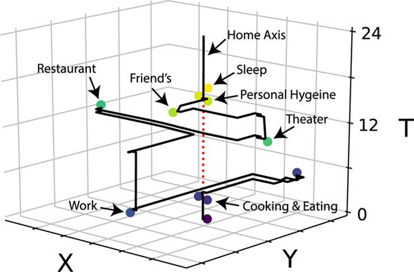
Here we demonstrate that it is possible to simulate activity trajectories (15) by using population level metrics. These can then be integrated with exposure profiles to estimate total human exposure. An activity trajectory, as illustrated in Figure 1, is defined as the time delimited pattern of activities a person engages in, along with relevant contextual information to describe the activity, including location and persons involved. Activity trajectories may also be called activity diaries or time use diaries when collected as part of a survey (16). There have been previous attempts to characterize human activity in this way to better understand exposure, such as the National Human Activity Pattern Survey (14), the Environmental Protection Agency’s (EPA) Consolidated Human Activity Database (17) and the National Household Travel Survey (18). Other studies of human activity tend to focus on a set of macro activities specific to the research subject, such as consumer activity or health oriented procedures (14, 19), or observation of micro-activities (e.g., all steps required to pour a cup of tea) in laboratory and clinical settings (20, 21), which are again non-generalizable.

Figure 1.

An example activity trajectory, which tracks the spatiotemporal path of a person through a 24 hour period. Time increases along the vertical axis, while the momentary position is captured in the XY plane. Each dot represents the start of a new activity. The dashed line represents the home axis, where the majority of personal activities are expected to occur.

We have developed the SpatioTemporal Human Activity Model, or STHAM, to generate and characterize travel trajectories and activity patterns (22–24) and to integrate exposure-agent geographical distributions to estimate total human exposure in large populations. The goal of this development is to have a model that can be applied by other scientists to better evaluate exposure in populations of interest. The STHAM consists of a semi-empirical agent based model (ABM) designed to generate probable activity trajectories for arbitrary populations and regions. An ABM simulates the activity of a group of complex entities or individuals using simple mathematical representations and have been successfully used to evaluate the emergent properties of rule based systems (25–27) including exposure related research (28–31).

Methods

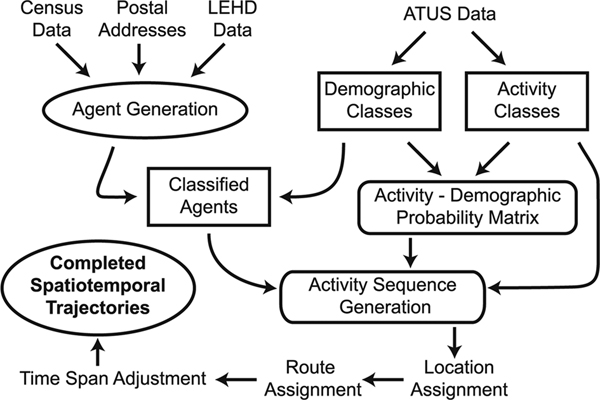
The STHAM initialization process is detailed in Figure 2. At the core of the STHAM is the agent, which is represented as a simple data record with demographic properties representing a hypothetical person. These properties (e.g. age, gender, census block location) are assigned to each agent randomly using the aggregate statistics at the census block level as constraints for the 2010 United States Census (32–34), so that the generated agents and the households to which they are assigned match the data provided in the census. Each household is then assigned a location in a round-robin fashion based on a list of physical postal addresses (35) that are matched to each census block. Next, each agent is assigned an employment status and, if relevant, an employment location, based on data from the Longitudinal Employee Household Dynamics Program (under the US Census Bureau) (LEHD) (36). The LEHD also provides an approximation for employment location at the census block level, which allows the model to simulate commuter patterns accurately. Finally, school participation is assigned using age and gender stratified enrollment rates from the American Community Survey (ACS) (33).

Figure 2.

The agent creation process. Demographic properties from the Census Block Tables are assigned to each agent, and then each agent is assigned to a household, which is given a home location. Additional locations for employment, school enrollment, and other regularly attended sites are then assigned. Household structure does not always accurately match actual structure because the structure is imputed.

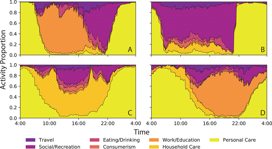
We have developed a simple unsupervised classification and sequence generation method from existing machine learning algorithms that is capable of generating coherent and stochastic sequences of activity from the data in the American Time Use Survey (ATUS) (16). A set of activity profiles were generated using the method described in detail in (37). Approximately 50–100 partially overlapping classes are generated for each classification. The overlap is due to the unsupervised nature of the algorithm and the high dimensionality of the ATUS dataset, but the classifier algorithms used to classify the activity classes still provides a sufficient level of class separation that usable classes can be isolated, as depicted in Figure 3. Next, a probability matrix is constructed mapping demographic class to activity class, so that daily activity patterns of an activity class can be stochastically assigned to each agent based on their demographic class. Separately, a random forest classifier is used to assign each agent to the appropriate demographic class, thereby connecting the agent demographic properties derived from the census data and household assignment to the appropriate daily activity patterns.

Figure 3.

Four example daily activity classifications identified from the American Time Use Survey. The vertical axis represents the relative proportion of each activity type, where each subplot is representative of a cohort of respondents from the ATUS who have similar patterns of activity as identified by our classification model. Class A represents the day of a typical working-class adult. It begins with sleeping, transitions into work, then recreation, and ends with sleep. Class B represents a day that primarily consists of recreation, whereas Class C represents a day that primarily consists of household care, which can include child care. Class D is similar to Class A, but consists of swing or night shift workers; this demonstrates that the classifier can differentiate both conceptual and temporal groupings of activities.

To obtain a list of useful consumer and business locations that are relevant for certain activity types (such as shopping and recreation), and to obtain a road network for travel planning we used the data provided by OpenStreetMap (38). The road network used is all roadways in the State of Utah as of January 2018, while trip routing is performed by the Open Source Routing Machine (38). Up to three routes are generated for each planned trip, with a weighted preference for the fastest route. The alternate routes, which are generated internally by the OSRM, are guaranteed to be different, and are locally optimal such that the travel time is comparable to the fastest route. Business locations were selected from locations that are currently tagged by OpenStreetMap as an office, shop, amenity, tourism, leisure, or sport location. When selecting a business for assigning an activity such as shopping or work, the fifty locations nearest to the current location of an agent are selected and weighted with a linear distribution. Importantly, these locations are treated in aggregate, with no effort being made to match the type of location to the context of the activity. The reason for this is that some activity types are underrepresented in the ATUS and have insufficient statistical power to infer the preferential location type, especially when the ATUS records are broken into subpopulations by the classifier. Additionally, the actual consumer facing function of a business is difficult to derive from the metadata provided by OpenStreetMap. Therefore, when a consumer oriented activity is performed in the simulation, it is assumed that the location selected reflects the activity being performed, even though the activity classification may be nonsensical when considering the actual function of the location.

Generating a coherent list of activities and their respective duration is a difficult problem because a sequence of activities encapsulates a complex decision process that is highly subject to externalities. Trajectories are generated independently, meaning there are no agent-agent interactions or other externalities that affect the trajectory generation beyond demographic class assignment, which implies that the activities of the agents are treated as independents in this study Agent-agent correlation is considered an additional complication that will be addressed in future work. Our method for generating activity trajectories relies on the start window concept developed in Ref. (37), which is a window of time where an activity can start. For each activity class we generate a set of independent start windows and a set of associated probability tables as described in previous work (37). For example, we would assign a daytime nap to a different activity window than we would for nighttime sleeping. For each activity class we generate a set of independent start windows and a set of associated probability tables.

After the calculation of the start windows, we construct prototype sequences stochastically, selecting for weekday or weekend behaviors. We generate trajectories for a single 24-hour period, starting at 4:00 AM, which is how the ATUS data is collected. We assign locations to each activity in the prototype, and then add travel activities in between activities with different locations. Each travel activity has a corresponding trajectory generated using the OpenStreetMap data and the OSRM, treating each waypoint in the planned route as a discrete new activity. The waypoints are generated automatically by the OSRM and contain an idealized travel time based on speed limits in addition to location. . At this stage, we have a complete activity trajectory, but the activity length generally needs adjusting to properly fill the 24-hour period. We adjust activity lengths so that activities stay within their start windows, adding additional activities as necessary to fill voids that cannot be covered by the selected activities. We recognize that this step introduces non-random errors into the sequence generation, but we consider it a compromise that allows us to create consistent activity trajectories.

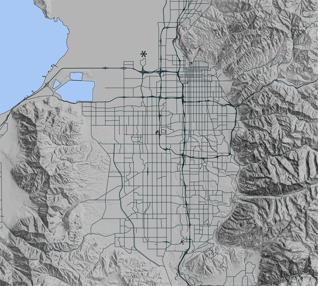
For this work, we have targeted the Wasatch Front (see Figure 4) and surrounding areas in the northern part of Utah, where the majority of the state’s population is located. Our overall test case simulates the activity of approximately 2.3 million people. The region is of particular interest due to the geographical phenomena of winter inversions, which contribute significantly to non-attainment of EPA air quality standards. The simulations presented in this paper covers a single 24-hour period on a typical weekday during an inversion. We obtained a stochastic model that estimates PM2.5 values based on known spatial and seasonal patterns (including inversions) from measured data from the Wasatch Front, which incorporates a daily sinusoidal cycle and elevation characteristics of the region, described in the supplemental material (See Table S1, Figure S1, Figure S2, Figure S3, Figure S4 ). This stochastic model was used to generate spatiotemporal matrices for estimating PM2.5 concentrations across the region of interest. We arbitrarily selected a day that showed a strong spatiotemporal variation to maximize the variation in calculated exposure when integrating the activity trajectories. This stochastic model uses a temporal scale of 1 hour and a spatial resolution of 250 meters. We performed additional detailed analysis on a subset of agent trajectories (approximately 1800) from our overall test case that were restricted to a small area near one of the PM2.5 measuring stations in Salt Lake City

Figure 4:

General topographic depiction of the Wasatch Front.

At this stage, we do not have an appropriate model for estimating PM2.5 from our model, so instead we have selected to use person-seconds as a surrogate metric for exposure. This does not allow us to calculate any practical exposure values, but it does allow us to estimate potential health impact from different classes of activities. We selected a 100 meter, 15 minute spatiotemporal resolution for estimating this impact, and split activities into three categories; travel activities, employment or work activities, and non-working or residential activities. We integrated the trajectories to obtain our person-second spatiotemporal matrix and then applied the Laplacian finite-difference method to estimate near field effects and simulate pollutant diffusion from activity in adjacent cells.

Some additional information on our simulation methods follows. The ATUS data used for this simulation comes from the 2015 release by the Bureau of Labor Statistics (37). Computing resources used for this research were provided by the Center for High Performance Computing at the University of Utah and typically consisted of 16-core Intel Xeon E5–2670 or 32-core AMD Opteron 6272 compute nodes using 64 or 256 GB of memory, depending on task. The model was written using Anaconda Python 3.6 (39) and utilizes the Pandas (40, 41) and Scikit-Learn (42) libraries. Execution of the model, including all preprocessing steps, can be generally completed in 1–2 weeks in its current form. The full code used in this work is publically available at https://github.com/uofu-ccts/prisms-comp-model-stham.

Results and Discussion

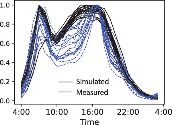
Validation of the STHAM is a moderately difficult problem, because we cannot directly measure activity trajectories at scale, and the model makes assumptions about household structure and activities that may introduce error into the resulting trajectories. A practical way to validate the STHAM is to use proxy measurements. Here we validated the model against traffic counts from the Utah Department of Transportation (UDOT) (25). We identified 20 roadway locations where the UDOT collected traffic counts where we could isolate traffic activity for independent roadways in our aggregate matrices. Since we can separate travel activities, here we used traffic counts from April 2014 to perform regressions against our simulated traffic counts on a selection of weekdays (all Wednesdays in April). The calculated average r-value of the regression for all locations is 0.938. We consider this to be strong proxy evidence that the STHAM is correctly capturing the diurnal cycle of activities and that reflects a reasonable approximation of the spatial distribution of activities. This is depicted in Figure 5, which shows normalized traffic rates for all measured locations. The overall shape of the simulated traffic is more rigid than the actual traffic counts, but generally follows the expected pattern of a strong peak in the morning and afternoon, reflecting the daily commute.

Figure 5.

A normalized comparison of the simulated traffic estimates against traffic count data obtained from the Utah Department of Transportation. Twenty geographical sites are compared using the average weekday counts from a single month. The simulated traffic rates have good correlation with the measured counts, with an r-value of 0.938, suggesting that the overall diurnal cycle is captured well.

We note that the absolute magnitude of simulated traffic counts (not shown) can vary by a factor of 0.76 to 1.16 compared to the measured traffic counts. Multiple factors contribute to this difference. The first main contributor is the absolute number of agents represented in the model; we modelled our agents based on the 2010 census, but modelled behaviors and commute patterns from 2015. The population in the Wasatch Front has increased by nearly 10% over this five-year period, meaning that our model underestimates the number of agents and total traffic. It also affects the regional distribution of population, since a cursory inspection of new housing and business development in that period indicates that it has occurred mostly in the South West corner of Salt Lake County, leading to a redistribution of traffic between recording locations. Second, the model fails to account for pass through traffic, freight activities, and site-to-site work traffic. We estimate this omission explains at least 50% of the difference in traffic counts. Third, we acknowledge that young children under the age of 15 are poorly represented in our model, because the ATUS does not have responses for respondents under the age of 15. We infer that school age children follow the activity profile of the typical high school student and toddlers and infants, we infer that their activities largely match those of their guardians and therefore simulate them as non-working adults. Finally, the route planning of our model does not take into account rush hour effects, and may select atypical and uncommon routes. These factors very likely explain the majority of variance in absolute traffic counts. Moreover, not simulating rush-hour effects may be an issue when developing the pollution component from the agent activities because congestion can exacerbate pollutant concentrations and exposure. Additionally, such congestion effects may disparately affect agents whose nature of work collocates them near high pollutant environments such as roadways.

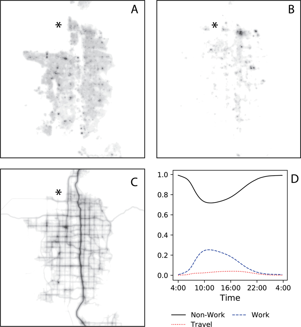
In Figure 6 we show the geospatial distribution of activities for three activity classes (non-working, working, and travel) at noon on a weekday, measured in person-seconds. The data shows marked differences between the categories, which combined with our socioeconomic knowledge of the region, demonstrates that agents are concentrated in areas corresponding to the types of activities being modelled. Panel A shows that non-working agents are concentrated in commercial districts where services or goods are offered. Because this category includes shopping and similar activities, this is not an unexpected outcome, but suggests that further diversification of this category is likely necessary in future refinements. Panel B shows similar hotspots for working agents, but concentrated in commercial and industrial districts, in particular the Salt Lake City downtown area in the north. Comparing Panels A and B in the northwest industrial district, we see that the area is completely devoid of non-working activity as expected, due to the total lack of housing and services in the area. Panel C, which shows the distribution of travel activities, effectively outlines the road network of Salt Lake County, and also shows the expected extra influence of busy traffic intersections. Animations of the full data can be found online at (Supplemental Materials Link for the supplementary GIFs files). Panel D of Figure 6 shows that a clear and obvious diurnal cycle is apparent in the relative activity weights, showing a peak in travel activity during 9:00 AM and 5:00 PM, when rush hour occurs. Likewise, working activities peak between 10:00 and 11:00 AM. The temporal distribution of activities is heavily weighted to non-working activities; this is expected because the majority of time is spent in non-working activities. However, it also shows that air pollution is disproportionally caused by a small fraction of human time expenditure. The Utah Department of Air Quality estimates that mobile emissions comprise approximately half of the primary and secondary sources of PM2.5 (43). Comparatively, the amount of time spent on travel activities that create emissions comprises less than 5% of human activity, showing a clear outsized effect from some activities. From this, we can extrapolate that some activities will have an outsized effect on human pollution exposure and provides impetus for us to diversify the categories that we sort activities into in the STHAM.

Figure 6.

The spatiotemporal distribution of human activities for the Salt Lake County Metropolitan area. Panels A-C show the geospatial distribution at noon on a typical weekday for Non-Working, Working, and Travelling activities, respectively. Each distribution is scaled independently and should not be compared directly. Panel D show the proportion of each activity category throughout the day.

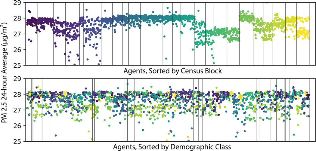
Figure 7 shows the results of integrating the activity trajectories across our stochastic PM2.5 model. The top panel shows the 24-hour average PM2.5 exposure values of each agent in a set of 23 adjacent census blocks. We selected a test case with substantial spatiotemporal variation on PM2.5, but we do not observe very much variation in the exposure levels for individual agents. Agents within each census block largely have the same average exposure as any other agent in the block, and excursions from the average are typically the result of travelling extreme distances from the assigned census block or encountering boundary conditions of the stochastic model. When we plot the hourly values for the entire cohort (not shown), we also find that PM2.5 exposure values have standard deviations under 3 μg/m², despite our expectation that there should be at least some excursion from the average. When we attempted to sort the agents by demographic class, we found that there was no obvious pattern or consistency in average exposure, as shown in the lower panel of Figure 7. From this result, we hypothesize that demographic class is only tangentially relevant to exposure, and that a more probable means for identifying cohorts of similar exposure is the census block assignment itself, or some other geographical features.

Figure 7.

Average daily 24-hour PM 2.5 exposure for a selected subset of agents, using a simple model for spatial PM2.5 values. The top panel sorts agents by census block, while the bottom sorts agents by demographic class. Colors correspond with census block assignment, with vertical lines indicating the transitions between groups. When sorted by census groups, a distinct pattern emerges from the data that is not present when sorting by demographic class. This reveals that exposure is more strongly correlated with spatial differences than demographic differences.

We compared the stochastic PM2.5 model to a self-consistent model of pollution concentration that assumes that individual exposure is tied to the sum of nearby human activity. Under this assumption the self-exposure can be measured in person-seconds. We made this comparison with the census block cohort, as well as a random sample of 10,000 agents. We examined these profiles by simple plotting to understand the characteristics of these profiles, and performing analyses to determine if distinctive patterns or clustering of patterns could be identified independent cohorts. When we plotted the 24-hour averages of the census block cohort using the self-consistent model we found similar spatial correspondence as we did with the simple PM2.5 model, with mean person-seconds being more strongly correlated to the census average block than with demographic class. However, we also found that the variance in person-seconds for each census block is 2–5 times larger than the PM2.5 model. Considering we were able to observe greater variation using the exact same set of activity trajectories, this shows that the STHAM self-consistent mode is able to capture features at smaller geographic levels than our PM2.5 statistical model, and implies that greater accuracy can be achieved from PM2.5 data modeled by the self-consistent model.

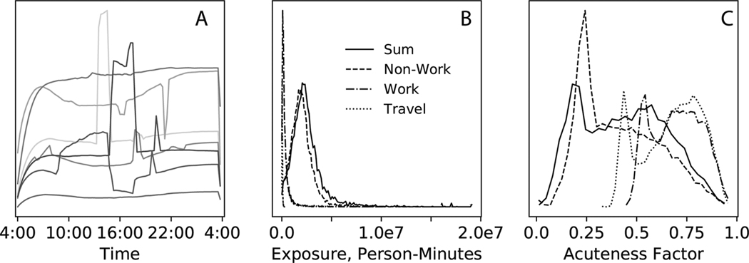
Our general finding of the sample of 10,000 agents is that there are no obvious or consistent patterns of exposure beyond diurnal variation and shared micro-environments. The measured person-second values are highly segmented; the segments are delimited by transitions between micro-environments, where the average person-seconds in each micro-environment can vary substantially in magnitude. This phenomenon can be seen in Figure 8, Panel A, where sudden and abrupt changes in values can be observed. We attempted to naively classify these activity trajectories based on the calculated person-second values, but found that there were no broad patterns that could be separated or identified; at best we were able to find a few instances of activity trajectories which had nearly identical temporal structure, but each sample was very small, with less than 10 trajectories per sample. This confirms our assertion that shared spatial environments are the best means for identifying at-risk cohorts.

Figure 8.

Exposure characteristics for the simulated population. Panel A shows a few example exposure profiles. The shapes of the profiles vary substantially and can be punctuated by abrupt changes in exposure. Panel B shows the distribution of total exposures in terms of person minutes, along with the distributions of relevant sub categories. Although work and travel activities have a smaller time contribution, we expect the health effects of actual pollution from these activities to be outsized in comparison to non-work activities. Panel C shows the distribution of acuteness factors, which is calculated by dividing the expected value of the exposure by the maximum value. A higher acuteness factor means that the total exposure is concentrated into a one or more high exposure events.

Considering that the spatial cohorts are the most similar with each other and that a large amount of variation exists in the census cohorts of the surrogate measures mode of the STHAM, we hypothesize that a more meaningful ways of characterizing at-risk groups is likely by measuring the total exposure in persons seconds, and by establishing a measure of acuteness. Acuteness is a dimensionless measure of how exposure is concentrated; an acuteness factor near 1.0 implies that the majority of total exposure is concentrated in a small amount of time, whereas an acuteness near 0.0 implies a uniform exposure across time. Figure 8, Panels B and C, show the distributions of total exposure and acuteness factors, respectively, using the surrogate measures as a basis for these calculations. Total exposure is distributed normally, with a long tail of high exposures, which holds true for all subcategories of activities. The highest total exposure in our sample of 10,000 agents is approximately 8 times the median exposure. Our hypothesis is that agents represented in the long tail likely experience chronic effects from the levels of exposure encountered. Acuteness appears to be bi-modally distributed, with a strong and narrow distribution in the lower range of acuteness values, and another broad distribution covering the full range of acuteness. Our analysis shows that this bimodality is a consequence of stationary and mobile agents having different overall patterns of exposure. Stationary agents do not experience abrupt changes in their microenvironment, and so they tend to have a more consistent exposure that only changes as the diurnal cycle proceeds, which consequently results in a low acuteness factor. Comparatively, mobile agents cross several microenvironments as they change locations, and can therefore experience acute exposure events. Exposure from work and travel activities tends to be more acute, which it is expected because these activities are more localized. These findings are consistent with previous results from Gurram et al. (29, 44). Future work will involve further characterization of total exposure and acuteness, and seeing if they have any correlation with incidence of respiratory conditions.

We define environmental context as the sum of the activities a person may be participating in or adjacent to, and the general environmental condition of the space a person occupies. A primary observation of this paper is that the environmental context that an individual experiences is strongly coupled to the exposures of that individual. As an example, a person, represented by an agent, who is cooking will be directly exposed to byproducts of the cooking process, but a person who is not participating in the cooking activity who is nearby will also be exposed. Additionally, an automated system, such as a furnace, can also alter exposure profiles without any human participation, and the latent PM2.5 levels inside a room can be drastically altered through air exchange with the outside environment. Consequently, the STHAM could benefit substantially from the incorporation of multi-agent activities and inter-agent interactions, where group activities and group adjacent activities are treated explicitly. This is especially true for the modeling of young children who are not autonomous, and who realistically have the same approximate activity trajectory and exposure as their primary guardian.

The development of an activity model for automated systems that function without human intervention also presents an area of potential interest that could complement the STHAM model well. A method for estimating the exposure and emission distributions of industrial and chemical processes that do not follow diurnal cycles is particularly important, but also technically difficult to obtain. On the other hand, good estimates for the emissions output from facilities engaged in such processes are available from regulatory agencies, such as the EPA CompTox database or Utah DAQ Air Quality Inventories. We plan on integrating these datasets with the STHAM to provide some means of estimating exposure from industrial sources.

The STHAM includes a significant empirical component due to the geographically constrained nature of exposure, and therefore relies on the availability of detailed geographic and demographic data. Importantly, the STHAM does not attempt to simulate the actual activities of people within the region of interest, but only simulates probable patterns of activity with high confidence that the model will capture typical modes of activity. Therefore, the model is only useful for examining possible activity profiles and aggregate population level contributions to air quality in general. However, with sufficient repetitions, the model can be used to identify at-risk populations that may not be identified through other means, and therefore has novel predictive value in estimating exposure burdens on different geographic groups.

An important limitation of this model is that the model is sensitive to the size of census blocks. Rural census blocks can be quite large in size, and population density can vary substantially, being concentrated in small townships or distributed across disperse areas. Postal addresses in rural areas can also include significant facilities such as mines, which may not house individuals but may be accidentally assigned a household. Therefore, when simulating rural regions, the household distribution needs to be sampled many more times to obtain reasonable estimates of activity. In addition, it is likely that rural areas need an entirely different exposure model, even if the STHAM can accurately represent the activities of a rural region, because of substantial differences in commercial and agrarian activities, and differences in regulatory mechanisms to limit pollution.

We have shown that the STHAM can provide insights into human activity patterns and spatio-temporal distributions of potential emission sources and while we used a distribution of particular matter derived from traffic as an example, the model can be used with any desired spatial temporal distribution of particle matter. The use of agent-based modelling coupled with the integration of public datasets and geographic information has the potential to yield exceptional insights into human exposure.

References

- 1.Brauer M, Hoek G, Smit HA, de Jongste JC, Gerritsen J, Postma DS, et al. Air pollution and development of asthma, allergy and infections in a birth cohort. European Respiratory Journal. 2007;29(5):879 LP-88. [DOI] [PubMed] [Google Scholar]
- 2.Anderson JO, Thundiyil JG, Stolbach A. Clearing the Air: A Review of the Effects of Particulate Matter Air Pollution on Human Health. Journal of Medical Toxicology. 2012;8(2):166–75. [DOI] [PMC free article] [PubMed] [Google Scholar]
- 3.Lu F, Xu D, Cheng Y, Dong S, Guo C, Jiang X, et al. Systematic review and meta-analysis of the adverse health effects of ambient PM2.5 and PM10 pollution in the Chinese population. Environmental Research. 2015;136:196–204. [DOI] [PubMed] [Google Scholar]
- 4.Hadlocon LS, Zhao LY, Bohrer G, Kenny W, Garrity SR, Wang J, et al. Modeling of particulate matter dispersion from a poultry facility using AERMOD. Journal of the Air & Waste Management Association. 2015;65(2):206–17. [DOI] [PubMed] [Google Scholar]
- 5.Colbeck I, Lazaridis M. Aerosols and environmental pollution. Naturwissenschaften. 2010;97(2):117–31. [DOI] [PubMed] [Google Scholar]
- 6.Apte JS, Messier KP, Gani S, Brauer M, Kirchstetter TW, Lunden MM, et al. High-Resolution Air Pollution Mapping with Google Street View Cars: Exploiting Big Data. Environmental Science & Technology. 2017;51(12):6999–7008. [DOI] [PubMed] [Google Scholar]
- 7.Mitchell LE, Crosman ET, Jacques AA, Fasoli B, Leclair-Marzolf L, Horel J, et al. Monitoring of greenhouse gases and pollutants across an urban area using a light-rail public transit platform. Atmospheric Environment. 2018;187:9–23. [Google Scholar]
- 8.Baker KR, Foley KM. A nonlinear regression model estimating single source concentrations of primary and secondarily formed PM2.5. Atmospheric Environment. 2011;45(22):3758–67. [Google Scholar]
- 9.Cyrys J, Pitz M, Bischof W, Wichmann HE, Heinrich J. Relationship between indoor and outdoor levels of fine particle mass, particle number concentrations and black smoke under different ventilation conditions. Journal Of Exposure Analysis And Environmental Epidemiology. 2004;14:275-. [DOI] [PubMed] [Google Scholar]
- 10.Lundrigan P, Min KT, Patwari N, Kasera SK, Kelly K, Moore J, et al. EpiFi: An In-Home Sensor Network Architecture for Epidemiological Studies. CoRR. 2017;abs/1709.02233. [Google Scholar]
- 11.Meseck K, Jankowska MM, Schipperijn J, Natarajan L, Godbole S, Carlson J, et al. Is missing geographic positioning system data in accelerometry studies a problem, and is imputation the solution? Geospatial health. 2016;11(2):403-. [DOI] [PMC free article] [PubMed] [Google Scholar]
- 12.Li Z, Che W, Frey HC, Lau AKH, Lin C. Characterization of PM2.5 exposure concentration in transport microenvironments using portable monitors. Environmental Pollution. 2017;228:433–42. [DOI] [PubMed] [Google Scholar]
- 13.Steinle S, Reis S, Sabel CE, Semple S, Twigg MM, Braban CF, et al. Personal exposure monitoring of PM2.5 in indoor and outdoor microenvironments. Science of The Total Environment. 2015;508:383–94. [DOI] [PubMed] [Google Scholar]
- 14.Klepeis NE, Nelson WC, Ott WR, Robinson JP, Tsang AM, Switzer P, et al. The National Human Activity Pattern Survey (NHAPS): a resource for assessing exposure to environmental pollutants. Journal Of Exposure Analysis And Environmental Epidemiology. 2001;11:231. [DOI] [PubMed] [Google Scholar]
- 15.Dias D, Tchepel O. Spatial and Temporal Dynamics in Air Pollution Exposure Assessment. Int J Environ Res Public Health. 2018;15(3). [DOI] [PMC free article] [PubMed] [Google Scholar]
- 16.Statistics USDoLBotL. American Time Use Survey, 2015 [United States]. 2016. [Google Scholar]
- 17.U.S. EPA. CHAD USER’S GUIDE: Extracting Human Activity Information from CHAD on the PC. In: Agency USEP, editor. Washington: 2002. [Google Scholar]
- 18.National Household Travel Survey 2020. [Available from: https://nhts.ornl.gov/.
- 19.Herder E, Siehndel P, Kawase R, editors. Predicting User Locations and Trajectories BT – User Modeling, Adaptation, and Personalization2014; Cham: Springer International Publishing. [Google Scholar]
- 20.Zhou Z, Chen X, Chung YC, He Z, Han TX, Keller JM. Activity Analysis, Summarization, and Visualization for Indoor Human Activity Monitoring. IEEE Transactions on Circuits and Systems for Video Technology. 2008;18(11):1489–98. [Google Scholar]
- 21.Redmond DP, Hegge FW. Observations on the design and specification of a wrist-worn human activity monitoring system. Behavior Research Methods, Instruments, & Computers. 1985;17(6):659–69. [Google Scholar]
- 22.Bradley M, Bowman JL, Griesenbeck B. SACSIM: An applied activity-based model system with fine-level spatial and temporal resolution. Journal of Choice Modelling. 2010;3(1):5–31. [Google Scholar]
- 23.Bhat CR, Guo JY, Srinivasan S, Sivakumar A. Comprehensive Econometric Microsimulator for Daily Activity-Travel Patterns. Transportation Research Record. 2004;1894(1):57–66. [Google Scholar]
- 24.Bellemans T, Kochan B, Janssens D, Wets G, Arentze T, Timmermans H. Implementation Framework and Development Trajectory of FEATHERS Activity-Based Simulation Platform. Transportation Research Record. 2010;2175(1):111–9. [Google Scholar]
- 25.ATR Hourly Volume Files, 2014. Utah Department of Transportation; 2015. [Google Scholar]
- 26.Pendyala RM, Kitamura R, Reddy DVGP. Application of an Activity-Based Travel-Demand Model Incorporating a Rule-Based Algorithm. Environment and Planning B: Planning and Design. 1998;25(5):753–72. [Google Scholar]
- 27.Arentze T, Hofman F, van Mourik H, Timmermans H. ALBATROSS: Multiagent, Rule-Based Model of Activity Pattern Decisions. Transportation Research Record. 2000;1706(1):136–44. [Google Scholar]
- 28.Brandon N, Dionisio KL, Isaacs K, Tornero-Velez R, Kapraun D, Setzer RW, et al. Simulating exposure-related behaviors using agent-based models embedded with needs-based artificial intelligence. Journal of Exposure Science & Environmental Epidemiology. 2018. [DOI] [PMC free article] [PubMed] [Google Scholar]
- 29.Gurram S, Stuart AL, Pinjari AR. Agent-based modeling to estimate exposures to urban air pollution from transportation: Exposure disparities and impacts of high-resolution data. Computers, Environment and Urban Systems. 2019;75:22–34. [Google Scholar]
- 30.Hatzopoulou M, Miller EJ. Linking an activity-based travel demand model with traffic emission and dispersion models: Transport’s contribution to air pollution in Toronto. Transportation Research Part D: Transport and Environment. 2010;15(6):315–25. [Google Scholar]
- 31.Beckx C, Int Panis L, Arentze T, Janssens D, Torfs R, Broekx S, et al. A dynamic activity-based population modelling approach to evaluate exposure to air pollution: Methods and application to a Dutch urban area. Environmental Impact Assessment Review. 2009;29(3):179–85. [Google Scholar]
- 32.2015 TIGER/Line Shapefiles (machine-readable data files). United States Census Bureau; 2015. [Google Scholar]
- 33.2015 American Community Survey (machine-readable data files). United States Census Bureau / American FactFinder; 2016. [Google Scholar]
- 34.2010 Censes demographic Profile summary File (machine-readable data files). United States Census Bureau / American FactFinder; 2011. [Google Scholar]
- 35.Utah Data (website). State of Utah; 2017. [Google Scholar]
- 36.2015 LEHD Origin-Destination Employment Statistics (LODES) Dataset Version 7.3 (machine-readable data files). United States Census Bureau; 2016. [Google Scholar]
- 37.Lund A, Gouripeddi R, Facelli J. Classification and Generation of Activity Sequences for Spatiotemporal Modeling of Human Populations. Peprint available at arXiv: http://arxivorg/abs/191105476. 2019. [DOI] [PMC free article] [PubMed] [Google Scholar]
- 38.Luxen D, Vetter C, editors. Real-time routing with OpenStreetMap data2011; New York: ACM. [Google Scholar]
- 39.Anaconda Python. Continuuum Analytics, Inc. (dba Anaconda, Inc.); 2017. [Google Scholar]
- 40.McKinney W. Pandas: a Foundational Python Library for Data Analysis and Statistics. [Google Scholar]
- 41.McKinney W, editor Data Structures for Statistical Computing in Python2010. [Google Scholar]
- 42.Pedregosa F, Varoquaux G, Gramfort A, Michel V, Thirion B, Grisel O, et al. Scikit-learn: Machine Learning in {P}ython. Journal of Machine Learning Research. 2011;12:2825–30. [Google Scholar]
- 43.Whiteman CD. Frequently asked Questions about Wintertime PM2.5 Pollution in Utah’s Salt Lake Valley. 2017. [Google Scholar]
- 44.Gurram S, Stuart AL, Pinjari AR. Impacts of travel activity and urbanicity on exposures to ambient oxides of nitrogen and on exposure disparities. Air Quality, Atmosphere & Health. 2015;8(1):97–114. [DOI] [PMC free article] [PubMed] [Google Scholar]
Associated Data
This section collects any data citations, data availability statements, or supplementary materials included in this article.