

Abstract
Stream fishes are restricted to specific environments with appropriate habitats for feeding and reproduction. Interactions between streams and surrounding landscapes influence the availability and type of fish habitat, nutrient concentrations, suspended solids, and substrate composition. Valley width and gradient are geomorphological variables that influence the frequency and intensity that a stream interacts with the surrounding landscape. For example, in constrained valleys, canyon walls are steeply sloped and valleys are narrow, limiting the movement of water into riparian zones. Wide valleys have long, flat floodplains that are inundated with high discharge. We tested for differences in fish assemblages with geomorphology variation among stream sites. We selected rivers in similar forested and endorheic ecoregion types of the United States and Mongolia. Sites where we collected were defined as geomorphologically unique river segments (i.e., functional process zones; FPZs) using an automated ArcGIS‐based tool. This tool extracts geomorphic variables at the valley and catchment scales and uses them to cluster stream segments based on their similarity. We collected a representative fish sample from replicates of FPZs. Then, we used constrained ordinations to determine whether river geomorphology could predict fish assemblage variation. Our constrained ordination approach using geomorphology to predict fish assemblages resulted in significance using fish taxonomy and traits in several watersheds. The watersheds where constrained ordinations were not successful were next analyzed with unconstrained ordinations to examine patterns among fish taxonomy and traits with geomorphology variables. Common geomorphology variables as predictors for taxonomic fish assemblages were river gradient, valley width, and valley slope. Significant geomorphology predictors of functional traits were valley width‐to‐floor width ratio, elevation, gradient, and channel sinuosity. These results provide evidence that fish assemblages respond similarly and strongly to geomorphic variables on two continents.
Keywords: fish assemblages, functional process zones, habitat, hydrogeomorphology, riparian, valley width
This study demonstrates the utility of spatial analysis in predicting functional process zones and fish assemblage variation in endorheic basins and forest steppe ecoregions of two continents.

1. INTRODUCTION
Abiotic variables are successful predictors of taxonomic and functional diversity of fishes in river ecosystems (Griffith et al., 2005; Rahel & Hubert, 1991; Seelbach et al., 2006). For example, geomorphological variables such as elevation and channel slope are correlated with fish occurrences in high elevation mountain streams (Kruse et al., 1997; Lanka et al., 1987). River habitats used by fishes vary with quantity and structure of woody debris and with substrate size and distribution that are linked to valley and riparian characteristics (Grant & Swanson, 1995). Steep slopes of constrained valleys contribute increased dead trees, boulders, and alluvial fans, while wide valleys contribute fewer boulders and trees, and increased abundances of herbaceous plants and shrubs on riparian banks. In steep‐sided, narrow (constrained) valleys, riparian vegetation is similar to the adjacent hill slope (Grant & Swanson, 1995; Merrill et al., 2006). In contrast, in wide valleys, riparian species are adapted to smaller substrates and frequent inundation by floodwaters (Naiman & Decamps, 1997). Although these valley types and riparian zones are distinctive based on interactions with river ecosystems, they contribute substrate material and debris that are utilized by aquatic biota as habitat.
The riverine ecosystem synthesis (RES; Thorp et al., 2006; Thorp et al., 2021) predicts that biotic and abiotic stream characteristics including fish assemblages should vary with functional process zones (FPZ). The RES defines FPZs as distinct, patchy, and discontinuous river segments with unique valley and reach scale characteristics (Thorp et al., 2006). Sources of FPZ variation include precipitation, elevation, valley morphology, stream gradient, and sinuosity. The RES differs from the river continuum concept (RCC) because it posits that river ecosystem function should be driven by primarily patchy geomorphological variation, rather by a predictable and continuous upstream to downstream gradient (Vannote et al., 1980).
Evidence that fish assemblages respond to geomorphology variation has been observed at both local stream reach scales (Rieck & Sullivan, 2020) and larger valley scales (Elgueta et al., 2019; Maasri et al., 2021). Elgueta et al. (2019) found that dominant fish assemblages at catchment, valley, and channel scales were associated with distinct FPZs. Additionally, variation in valley‐scale geomorphology was a strong predictor of taxonomic fish assemblages for Mongolia forest steppe and grassland rivers (Maasri et al., 2021). Maasri et al. (2021) compared fish assemblage variation among reaches defined by geomorphology using occurrence‐ and abundance‐based beta diversities. Classification of fishes by functional traits frequently provides additional information about ecosystem roles in fish assemblage analyses (Pease et al., 2012). Robbins and Pyron (2021) identified three unique FPZs based on variation in channel width, floodplain width, and down valley slope for the mainstem of the Wabash River, USA. Significant differences in taxonomic and functional fish assemblages were found among FPZs and with river location (distance from confluence), supporting both the RCC and RES. However, variation of fish assemblages with hydrogeomorphology is largely unknown for forested and endorheic mountain streams of United States and Mongolian river ecosystems.
While mountain streams may represent rivers that inspired the RCC—rivers with montane headwaters that increase in volume with downstream distance (Vannote et al., 1980)—mountain rivers of endorheic regions likely have different functions. Endorheic rivers are confined to a drainage area and terminate in saline lakes (Great Salt Lake, Utah) or sink formations (Carson Sink, Nevada) (Benke & Cushing, 2011; Sigler & Sigler, 1987). Endorheic basin ecoregions are arid to semi‐arid drainages where rivers terminate in saline lakes or sink formations and eventually evaporate (Abell et al., 2008; Nichols, 2007). These ecoregions also tend to have low fish species richness in lotic habitats due to geographic isolation, but can have high endemism in lake and spring ecosystems (Probst et al., 2020; Sigler & Sigler, 1987). The limited dispersal ability of fishes to and from endorheic rivers, paired with low diversity and higher sensitivity to water withdrawal in desert ecoregions, further results in Great Basin fish assemblages that are highly sensitive to climate change (Jaeger et al., 2014).
The objectives of this study were to evaluate geomorphological variables as predictors of variation in mountain stream fish assemblages for forested and endorheic river ecosystems. Our hypothesis was that fish assemblages defined by taxonomy and functional traits will vary with geomorphology variables. We selected mountain watersheds in western United States and Mongolia to provide contrasts in human impacts. Western US rivers are impacted by dams, water diversions, agriculture management activities, and invasive species. Mountain rivers of Mongolia have few or no dams or water diversions or invasive species, and over‐grazing by livestock is the only agricultural impact (Altanbagana & Chuluun, 2010).
2. METHODS
2.1. Watershed and site selection
We used the ArcGIS‐based geomorphic model RESonate to identify distinctive reaches or FPZs separately in Mongolia and western North America mountain and endorheic ecosystems, following Williams et al. (2013) and Maasri et al. (2021). This is a GIS approach to identify unique river reaches using variables that are available in online GIS. We extracted geomorphic variables at 10‐km intervals, including the following: elevation, mean annual precipitation, geology, valley width, valley floor (floodplain) width, valley width‐to‐valley floor width ratio, river channel sinuosity, right valley slope, left valley slope, and down valley slope (Appendix 1). Data were normalized to a 0–1 scale, and a dissimilarity matrix was generated using a Gower dissimilarity transformation (Gower, 1971). The Gower transformation is recommended for nonbiological data when the measures are range‐standardized (Thoms et al., 2018). The dissimilarity matrix was used in a hierarchical clustering following the Ward linkage method, as it provided the best partitioning of cluster groups (Murtagh & Legendre, 2014). Additionally, we used a principal component analysis (PCA) to identify the contributive variables most important for group partitioning and to describe the cluster groups based on the ten variables identified above. Groups of 10‐km river sections, constituting discrete FPZs, were later mapped to allow for the identification of fish collection sites (Figure 1).
FIGURE 1.

Rivers of the United States (top) and Mongolia (bottom) endorheic (T) and forested (FS) ecoregions
We performed the clustering using the cluster package (version 2.1.0; Maechler et al., 2018) and the PCA using the FactoMineR package (version 1.42; Lê et al., 2008) in R version 3.6.3 (Team R Core, 2020). We mapped the resulting groups using ArcGIS (version 10.5) (Figure 1).
2.2. Fish collections
We established reaches for fish collections measuring 20 times the mean wetted width of the river, calculated independently for each site. Fishes were collected by single‐pass backpack electrofishing with two netters (Ball State University IACUC #126193) following the American Fisheries Society standard collection protocols CPUE (Bonar et al., 2009). Electrofishing surveys were supplemented with seine netting and snorkel surveys when electrofishing was not possible due to low water conductivity for six headwater US Forested watershed sites. Seine netting resulted in fewer than one individual fish per site on average and was discontinued after collecting in US endorheic rivers. Snorkel surveys were performed in six headwater streams where water conductivity was too low for electrofishing. Snorkeling consisted of slowly swimming upstream for the site distance and recording all observed fishes. Fishes were identified to species, weighed to the nearest 0.01 g, measured in standard length (mm), and released. Fish species identifications and functional traits were from Mendsaikhan et al. (2017) for Mongolia or Poff and Allen (1995) for United States, and reproductive traits were from Balon (1975). Traits were substrate and stream size preferences, reproductive traits, and trophic traits.
2.3. Fish assemblage analyses
We evaluated fish assemblage responses to geomorphology using constrained ordinations with forward selection of environmental variables in CANOCO 5 software (canoco5.com). CANOCO evaluates length of the first ordination axis and recommends either a linear method (redundancy analysis, RDA) or a nonlinear method (canonical correspondence analysis, CCA). RDA is a direct gradient technique for multifactorial analysis of variance models using ecologically relevant distance measures and significance testing of individual variables (Legendre & Anderson, 1999). CCA is a direct gradient weighted averaging regression technique in CANOCO using environmental predictors (Palmer, 1993). Analyses were conducted for each ecoregion separately, and geomorphology data were reduced into fewer dimensions using principal components analysis (PCA) in Minitab version 18. Subsequent PCA axes were entered into RDA or CCA as environmental predictors of fish assemblage variation. If CANOCO was unable to reach a solution for constrained ordinations, we used unconstrained ordinations with environmental variables projected. CANOCO suggests either a linear PCA or unimodal (correspondence analysis) ordination based on gradient length. Fish and abundances by traits were log‐transformed by log (X + 1) before analysis to account for abundances spanning three orders of magnitude. We eliminated hybrid tiger trout from analyses as they were introduced and not capable of reproducing.
3. RESULTS
3.1. Geomorphological analysis
Functional process zones were classified using nine geomorphology variables and precipitation. Using the hierarchical method, four or five FPZs were defined for each river basin (Figure 1). The strongest contributing variables for FPZ delineation were valley width, elevation, and valley floor width. Geomorphology variables were reduced into PCA axes for each ecoregion and resulting PC axes by ecoregion were unique. US endorheic rivers were the Carson, Humboldt, and Bear rivers of the Great Basin ecoregion of the southwestern United States (n = 23 sites; Figure 1). US rivers were Tongue, Powder, and Ten Sleep rivers in the mountain ecoregions of the Yellowstone River watershed (Wyoming, US; n = 20 sites; Figure 1). Mongolian forested rivers were on the Eg River and Delgermurun rivers of north‐central Mongolia (n = 12 sites; Figure 1). Mongolia endorheic rivers were the Khovd and Zavkan rivers of western Mongolia (n = 13 sites; Figure 1). Site length varied from 40 to 1,500 m with a mean of 290 (SD = 266) m.
3.2. Fish assemblages
Fourteen of 19 species in the US endorheic ecoregion were invasive, and three of four species in the US forested ecoregion were invasive (Table 1). No invasive species were collected among the seven species from the Mongolia mountain ecoregion, or the five species from the Mongolia endorheic ecoregion (Table 1). Mean species richness (± SD) per site for the US endorheic ecoregion was 4.1 (± 2.1), 2.1 (± 0.8) for the US forested ecoregion, 2.7 (± 1.2) for the Mongolia endorheic ecoregion, and 3.9 (± 1.3) for the Mongolia forested ecoregion. Mean abundances (± SD) per site for the US endorheic ecoregion were 100 (± 113), 40 (± 29) for the US forested ecoregion, 97 (± 82) for the Mongolia forested ecoregion, and 59 (± 54) for the Mongolia endorheic ecoregion. We collected one endemic species in the US endorheic ecoregion (Tahoe sucker Catostomus tahoensis), one in the Mongolia endorheic ecoregion (Golubtsovi's stone loach, Barbatula golubtsovi), and one in the Mongolia forested ecoregion (Siberian dace, Leuciscus leuciscus).
TABLE 1.
Fishes collected by country and ecoregion
| Species | Common name | Country | Ecoregion | n |
|---|---|---|---|---|
| Rhinichthys osculus | Speckled dace | US | Endo | 449 |
| Pimephales promelas | Fathead minnow* | US | Endo | 280 |
| Catostomus tahoensis | Tahoe sucker | US | Endo | 271 |
| Salvelinus fontinalis | Brook trout* | US | Endo | 227 |
| Cottus beldingii | Paiute sculpin | US | Endo | 220 |
| Lepomis cyanellus | Green sunfish* | US | Endo | 205 |
| Micropterus dolomieu | Smallmouth bass* | US | Endo | 169 |
| Cyprinus carpio | Common carp* | US | Endo | 140 |
| Salmo trutta | Brown trout* | US | Endo | 84 |
| Oncorhynchus mykiss | Rainbow trout* | US | Endo | 71 |
| Ameirus melas | Black bullhead* | US | Endo | 57 |
| Oncorhynchus clarki utah | Bonneville cutthroat trout | US | Endo | 43 |
| Gambusia affinis | Mosquitofish* | US | Endo | 23 |
| Catostomus platyrhynchus | Mountain sucker | US | Endo | 16 |
| Lepomis macrochirus | Bluegill sunfish* | US | Endo | 16 |
| Prosopium williamsoni | Mountain whitefish | US | Endo | 7 |
| Rhinichthys cataractae | Longnose dace | US | Endo | 3 |
| Richardsonius egregius | Lahontan redside | US | Endo | 3 |
| Micropterus salmoides | Largemouth bass* | US | Endo | 2 |
| Salmo trutta | Brown trout* | US | For | 215 |
| Salvelinus fontinalis | Brook trout* | US | For | 203 |
| Oncorhynchus clarki bouvieri | Yellowstone cutthroat trout | US | For | 107 |
| Oncorhynchus mykiss | Rainbow trout* | US | For | 46 |
| Barbatula barbatula | Stone loach | Mongolia | Endo | 460 |
| Thymallus brevirostris | Mongolian grayling | Mongolia | Endo | 110 |
| Barbatula conilobus | Conilobus’ stone loach | Mongolia | Endo | 109 |
| Oreoleuciscus potanini | Altai osman | Mongolia | Endo | 89 |
| Barbatula golubtsovi | Golubtsovi's stone loach | Mongolia | Endo | 2 |
| Phoxinus phoxinus | Common minnow | Mongolia | For | 845 |
| Brachymystax lenok | Lenok | Mongolia | For | 98 |
| Barbatula barbatula | Stone loach | Mongolia | For | 85 |
| Thymallus arcticus | Arctic grayling | Mongolia | For | 34 |
| Leuciscus leuciscus | Common dace | Mongolia | For | 13 |
| Esox lucius | Northern pike | Mongolia | For | 4 |
| Perca fluviatilis | European perch | Mongolia | For | 1 |
Endo designates the endorheic basins and for the forested basins. Asterisks * refer to invasive species.
3.3. US forested ecoregion
CANOCO recommended a unimodal ordination (CCA) based on gradient of 3.3 SD units for the US forested taxonomy data. The CCA ordination for the US forested ecoregion using taxonomy resulted in two axes that explained 35.2% and 31.1% of variation (Figure 2). The forward selection procedure in the CCA resulted in only geomorphology PC3 as significant; this PC axis was driven by river channel sinuosity, elevation, and gradient (Table 2). The CCA first axis was significant (F = 2.3, p = .022), and all CCA axes together were significant (F = 4.1, p = .008; Table 2). Brook trout and Yellowstone cutthroat trout occurred at higher elevations, with decreased channel sinuosity compared to rainbow trout and tiger trout. Brown trout tended to occur in streams with wider valleys and increased annual precipitation.
FIGURE 2.

Canonical correspondence analysis ordination of fishes by taxonomy for US forested ecoregion. Top figure is sites; bottom figure is species and vectors for the significant predictor. Sites are labeled by functional process zone
TABLE 2.
Results for constrained ordination analyses of fishes by ecoregion, by taxonomy and functional traits
| Ecoregion | Contribution % | Pseudo‐F | p (adj) |
|---|---|---|---|
| US forested taxonomy | |||
| PC3: elevation, gradient, − river channel sinuosity | 66.5 | 7.1 | .018 |
| PC2: valley width, precipitation | 25.9 | 4.1 | .021 |
| US endorheic taxonomy | |||
| PC1: − gradient, + left valley slope, valley width‐to‐floor width ratio | 47.7 | 2.8 | .006 |
| Mongolia endorheic traits | |||
| PC2: valley width‐to‐floor width ratio, gradient, precipitation | 51.8 | 5.4 | .048 |
| PC3: − channel sinuosity, − valley width, left valley slope | 44.4 | 7.3 | .018 |
CANOCO recommended a linear ordination (RDA) based on gradient of 1.1 SD units for the US forested trait data. The RDA ordination for the US forested ecoregion using traits did not result in a significant result. The unconstrained ordination selected was PCA with projection of environmental variables, because the gradient was 1.0 SD long. The first PCA axis explained 56.1% of variation, and the second PCA axis explained 24.4% of variation. Variation explained by the environmental variables was 17.0% on the first axis and 7.1% on the second axis, and PC3 was strongly correlated with the first and second axis (Figure 3). PC3 explained elevation and river channel sinuosity variation, with positive loadings for sites with higher elevation and increased sinuosity. PC1 explained valley floor width with negative loadings for sites with lower valley floor widths. Fishes that are lithophils (reproductive mode 9, bury their eggs in gravel) that are piscivores with preferences for montane streams with all substrates except for sand, clay/silt, boulder, and cobble, occurred at sites with higher elevation and increased channel sinuosity.
FIGURE 3.
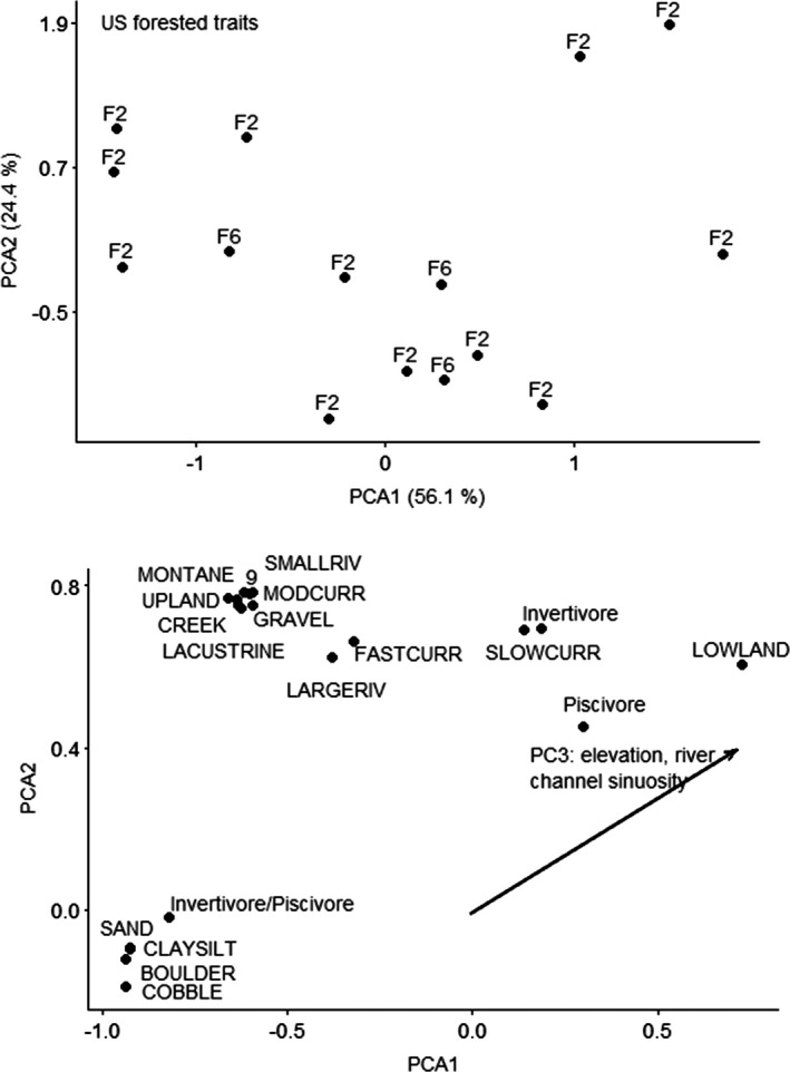
Principal components analysis ordination of fishes by traits for US forested ecoregion. Top figure is sites; bottom figure is species and vectors for the significant predictor. Sites are labeled by functional process zone. Trait numbers refer to reproduction mode
3.4. US endorheic ecoregion
Response data resulted in a gradient of 7.8 SD units; thus, we used a nonlinear ordination (CCA). The CCA ordination for the US endorheic ecoregion using taxonomy resulted in first two axes that explained 10.2% and 20.1% of variation (Figure 4). The forward selection procedure resulted in geomorphology PC1 as a significant predictor. PC1 represents gradient, left valley slope, and valley width‐to‐floor width ratio. The CCA first axis was not significant, but all axes together were significant (F = 1.7, p = .014). Sites with higher gradients, higher valley slope, and higher valley width‐to‐floor width ratio had higher abundances of brown trout and tiger trout, and lower abundances of other species.
FIGURE 4.

Canonical correspondence analysis ordination of fishes by taxonomy for US endorheic ecoregion. Top figure is sites; bottom figure is species and vectors for the significant predictor. Sites are labeled by functional process zone
CANOCO recommended a linear method (RDA) based on gradient of 1.5 SD units for the US endorheic traits data. None of the predictor variables were significant in the RDA ordination for US endorheic ecoregion using traits. The unconstrained ordination selected was PCA with projection of environmental variables, because the gradient was 1.4 SD long. The first PCA axis explained 49.7% of variation, and the second PCA axis explained 20.4% of variation. Variation explained by the environmental variables was 4.5% on the first axis and 10.7% on the second axis, and PC1 was strongly correlated with the first and second axes (Figure 5). PC1 explained left valley slope and valley width‐to‐floor width ratio, with positive loadings for sites with higher slopes and higher valley width‐to‐floor width ratios. Sites with higher valley slope and increased valley width‐to‐floor width ratios had fishes with reproductive modes of lithophils (reproductive mode 9, bury their eggs in gravel) or nest spawners (reproductive mode 22, build structures for egg deposition) that were invertivore/piscivores and prefer streams with fast current and boulder substrates.
FIGURE 5.

Principal components analysis ordination of fishes by traits for US endorheic ecoregion. Top figure is sites; bottom figure is species and vectors for the significant predictor. Sites are labeled by functional process zone. Trait numbers refer to reproduction mode
3.5. Mongolia endorheic ecoregion
CANOCO recommended a linear method (RDA) based on gradient of 2.3 SD units for the Mongolia endorheic taxonomy data. None of the predictors for the RDA ordination for the Mongolia endorheic ecoregion fish by taxonomy were significant. The unconstrained ordination selected was PCA with projection of environmental variables, because the gradient was 1.8 SD long. The first PCA axis explained 52.5% of variation, and the second PCA axis explained 25% of variation. Variation explained by the environmental variables was 18.8% on the first axis and 15.6% on the second axis. PC2 was strongly correlated with the first and second axes, and PC3 was correlated with the first axis (Figure 6). PC2 explained valley width‐to‐floor width ratio, with positive loadings for sites with higher valley width‐to‐floor width ratios. PC3 explained left valley slope and river channel sinuosity, with positive loadings for sites with higher slope and decreased sinuosity. Mongolia grayling occurred at sites with higher valley width‐to‐floor width ratios compared to other species. Barbatula conilobus loaches occurred at sites with higher valley slope and increased channel sinuosity compared to other species.
FIGURE 6.
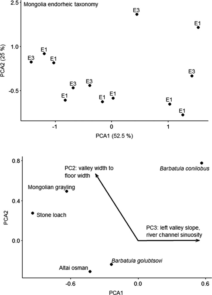
Principal components analysis ordination of fishes by taxonomy for Mongolia endorheic ecoregion. Top figure is sites; bottom figure is species and vectors for the significant predictor. Sites are labeled by functional process zone
CANOCO recommended a linear method (RDA) based on gradient of 1.2 SD units for the Mongolia endorheic traits data. The RDA ordination for the Mongolia endorheic ecoregion using traits resulted in two axes that explained 50.2% and 11% of variation (Figure 7). The forward selection procedure resulted in PC2 and PC3 as significant. PC2 was driven by valley width‐to‐floor ratio, stream gradient, and precipitation, and PC3 was driven by channel sinuosity, valley width, and valley slope. The RDA first axis was significant (F = 3.0, p = .014), and all RDA axes were significant (F = 5.2, p = .006). Fishes with reproductive modes of pelagolithophils (reproductive mode 3, deposit eggs on rocks or gravel bottom, in some larvae become buoyant) or lithophils (reproductive mode 4, deposit eggs rock or gravel) that were invertivore/algivores and prefer vegetation, gravel, and sand substrates and multiple current velocities and stream sizes occurred at sites with higher valley width‐to‐valley floor ratios, higher gradients, and increased annual precipitation. Fishes with reproductive mode of phytolithophils (reproductive mode 6, deposit eggs in clear water on plants or other submerged items) that were omnivores or invertivores, and prefer boulder and bedrock substrates with silt, and slow current occurred at sites with decreased channel sinuosity and decreased valley slope.
FIGURE 7.

Ordination (RDA) of fishes by traits for Mongolia endorheic ecoregion. Top figure is sites; bottom figure is species and vectors for the significant predictor. Sites are labeled by functional process zone and trait numbers refer to reproduction mode
3.6. Mongolia forested ecoregion
CANOCO recommended a linear method (RDA) based on gradient of 2.1 SD units for the Mongolia forested taxonomy data. CANOCO recommended a linear method (RDA) based on gradient of 1.9 SD units for the Mongolia forested traits data. Neither of the RDA ordinations for the Mongolia forested ecoregion fish by taxonomy or traits resulted in significant predictors. The unconstrained ordination selected for taxonomy data was PCA with projection of environmental variables, because the gradient was 1.8 SD long. The first PCA axis explained 55.7% of variation, and the second PCA axis explained 19.3% of variation. Variation explained by the environmental variables was 8.2% on the first axis and 6.5% on the second axis. PC1 was strongly correlated with the second axis, and PC3 was correlated with the first and second axes (Figure 8). PC1 explained valley width‐to‐floor width ratio, with positive loadings for sites with lower valley width‐to‐floor width ratios. PC3 explained right valley slope and elevation, with positive loadings for sites with higher slope and lower elevation. Sites with higher elevation, higher slopes, and higher valley width‐to‐valley floor width ratios had higher abundances of northern pike compared to other species.
FIGURE 8.

Principal components analysis ordination of fishes by taxonomy for Mongolia forested ecoregion. Top figure is sites; bottom figure is species and vectors for the significant predictor. Sites are labeled by functional process zone
The unconstrained ordination selected for trait data was PCA with projection of environmental variables, because the gradient was 1.7 SD long. The first PCA axis explained 76.5% of variation, and the second PCA axis explained 12.7% of variation. Variation explained by the environmental variables was 7.7% on the first axis and 9.1% on the second axis. PC1 was strongly correlated with the first axis, and PC3 was correlated with the first and second axes (Figure 9). PC1 explained valley width‐to‐floor width ratio, with positive loadings for sites with lower valley width‐to‐floor width ratios. PC3 explained right valley slope and elevation, with positive loadings for sites with higher slope and lower elevation. Fishes with reproductive modes of phytophils (reproductive mode 7, scatter eggs with an adhesive membrane that sticks to plant or logs) or lithophils (reproductive mode 4, deposit eggs rock or gravel) that were piscivores or omnivores that prefer multiple substrates had higher abundances at sites with increased valley slopes and increased valley width‐to‐valley floor width ratios.
FIGURE 9.

Principal components analysis ordination of fishes by traits for Mongolia endorheic ecoregion. Top figure is sites; bottom figure is species and vectors for the significant predictor. Sites are labeled by functional process zone and trait numbers refer to reproduction mode
4. DISCUSSION
4.1. Effects of geomorphology on fish assemblage structure
Our results showed that geomorphology has a strong influence on fish assemblages in US forested and endorheic rivers and in Mongolia endorheic rivers, confirming recent results showing how changes in valley‐scale geomorphology drives changes in fish assemblages in river macrosystems (Maasri et al., 2021). Geomorphic variables that were important in predicting fish occurrences tended to distinguish reaches based on valley width and gradient. However, the variables that were significant varied among ecoregions and whether we used fishes classified by taxonomy or by functional traits. Our interpretation is that depauperate fish assemblages of ecoregions resulted in low ability to explain variation using geomorphology.
At fine scales, habitat type, complexity, and hydrological regime dictate the presence of many stream organisms. However, at coarse scales, riparian vegetation, nutrient loading, and establishment of nonindigenous species contribute the largest effect on fish assemblage variation (Hermoso et al., 2011; Schlosser, 1991). However, anthropogenic alteration of river habitats, including drainage of wetlands and forests for row crop agriculture, channelization, and snag removal for the facilitation of barge traffic, and the erection of impoundments for flood control and retention of usable water have widespread effects on natural community assemblages (Nilsson et al., 2005). Fishes in high elevation mountain stream ecosystems are currently restricted by fewer anthropogenic variables than fishes in lower elevation rivers (e.g., upstream of dams and nonpoint source pollutants). However, historic alterations such as beaver removal and mining in the mountain steppes of the western United States resulted in incision of stream channels and contamination by heavy metals (Wohl, 2006). The majority of fishes in this region are stocked or re‐introduced by state agencies, impairing the biotic integrity of local ecosystems. Conversely, in Mongolia, forested steppe rivers are not altered through large impoundments or stocking of native or non‐native species, but they are impacted by widespread and intensive livestock grazing and mining activities (Chalov et al., 2012). Future alterations to Mongolian rivers are currently in planning stages and include the installation of high‐head dams and introductions of exotic salmonid and centrarchid species for recreational fishing (Simonov et al., 2017).
Our results suggest that valley width and gradient are effective predictors of assemblage variation and species occurrence in mountain rivers. Riparian zones of rivers link valley width to river ecosystem characteristics and are strongly influenced by valley characters (Merrill et al., 2006). Riparian contributions to physical stream features include additions of organic material, woody debris, and indirectly control of nutrient inputs (Gregory et al., 1991). Valley geomorphology influences the composition of substrates and the way in which material is deposited in the river. The width of a valley can influence the rate at which this material is deposited into lotic ecosystems (Leopold et al., 1964), resulting in distinctive fish habitat features. Walters et al. (2003) found this for Piedmont streams when they compared fish assemblages among sites with different reach characteristics.
Fish assemblage variation in constrained and wide valleys can result through four possible mechanisms. First, substrate variation may strongly influence fish assemblages (Mueller & Pyron, 2010); constrained valley rivers generally have higher velocity water and larger substrates than wide valley rivers. These larger substrates in constrained valleys contribute to the availability of a second potential mechanism contributing to the organization of fish assemblages: fish habitat and cover (Stefferud et al., 2011). Constrained valley rivers substrates tend toward large cobble, boulders, and logjams that are sourced from the valley slope and provide important for fish cover, whereas wide valley rivers frequently contain increased riparian vegetation and macrophytes likely due to overall lower water velocities and decreased abundance of large woody debris due to their gradually sloping banks. A third mechanistic category for valley width control on fish assemblages is food web variation (Smits et al., 2015). Less direct sunlight reaches rivers in constrained valley rivers compared to wide valley rivers. This is expected to result in lower primary productivity and variation in basal carbon sources. A fourth mechanistic category for valley width control on fish assemblages is competitive interaction among fish species. Survival and recruitment of smaller forage fishes varies in the presence of dominant predators or available resources in a stream reach. We suggest that all four of these mechanisms contribute to the observed variation in fish assemblages mediated by valley width.
The US Great Basin contains several species of endemic pupfishes and suckers, as well as the Lahontan and Bonneville subspecies of cutthroat trouts (Onchorhynchus clarki). Multiple fish introductions and experimental fisheries near the end of the 19th and first part of the 20th century occurred in this ecoregion, starting with overfishing of native species, then introductions of numerous invasive species including common carp (Cyprinus carpio), smallmouth bass (Micropterus dolomieu), brown trout (Salmo trutta), and black bullhead (Ameiurus melas) (Sigler & Sigler, 1987). To further evaluate the validity of these valley width associations, we compared published habitat preferences of species in Table 1 to habitat variables associated with valley type from our collections. Cunjak and Green (1983) found that rainbow trout (Oncorhynchus mykiss) inhabit higher velocity streams than brook trout. Brown trout are described as a habitat generalist (Ayllón et al., 2010) although Vismara et al. (2001) found that adult brown trout in Italian rivers preferred habitats with large boulders and overhanging vegetation. Although we found the highest abundances of rainbow trout and brook trout in constrained valleys, our observations during snorkel surveys showed these taxa inhabit different microhabitats. Speckled dace (Rhinichthys osculus) inhabit faster moving waters than other desert species (Scoppettone et al., 2005) and adults utilize large stones as cover (Peden & Hughes, 1981). We found the highest abundances of speckled dace in constrained valleys with high water velocity. Adult Tahoe sucker prefer large substrates (Moyle & Vondracek, 1985), which is consistent with constrained valley habitats where we found them. Adult cutthroat trout habitat is characterized by overhanging vegetation and availability of pool habitat (Kruse et al., 2000), similar to habitats in wide valleys where we collected them. Other native species occurred in wide valley habitats as predicted: common minnow prefer relatively shallow, slow‐moving lotic habitats but do not have preferences for substrate size (Lamouroux et al., 1999). Mountain sucker (Catostomus platyrhynchus) inhabit riffles and fast water habitats with substrates ranging from sand to boulders (Sigler & Sigler, 1987). Detailed valley type habitat preferences are not available for Mongolia fishes.
The invasive species we collected did not occur in predicted patterns for constrained vs. wide valley habitats. Fathead minnow are generalists and are associated with pool and backwater habitats (Quist et al., 2005). Black bullhead are considered effective invasive species due to their status as habitat generalists for feeding and reproduction (Novomeská & Kováč, 2009), although they prefer aquatic vegetation cover (Stuber, 1982). Western mosquitofish (Gambusia affinis) prefer calm water over fast‐moving rivers (Casterlin & Reynolds, 1977) and inhabit a wide range of habitats (Pyke, 2005). Three invasive species occurred in habitats as predicted for wide valleys. Common carp occur in slow‐moving waters with small substrates (Butler & Wahl, 2010. Smallmouth bass and green sunfish are invasives that are strongly associated with large substrates, boulders, large woody debris, and root wads in slow‐moving stream habitats (Stuber et al., 1982; Todd & Rabeni, 1989).
Each of these habitat and hydrology preferences are concordant with habitat variation that is expected to characterize valley types. Species that prefer faster water and large substrates frequently occur in constrained valley reaches, while species that prefer slower flows or algae and macrophyte growth occur in wide valley reaches. These results may not be applicable across ecoregions or river drainages, but our method of river classification can be implemented in any lotic habitat requiring decisions for stocking success or conservation of fish species. This study demonstrates the utility of spatial analysis in predicting functional process zones and fish assemblage variation in endorheic basins and forest steppe ecoregions of two continents. Future research should evaluate associations of habitat type with valley width and fish preferences for habitat in each ecoregion.
CONFLICT OF INTEREST
None declared.
AUTHOR CONTRIBUTIONS
Robert Shields: Conceptualization (lead); Data curation (equal); Formal analysis (lead); Investigation (equal); Methodology (equal); Writing‐original draft (lead). Mark Pyron: Conceptualization (equal); Data curation (lead); Funding acquisition (equal); Investigation (lead); Methodology (equal); Project administration (equal); Writing‐original draft (equal). Emily R. Arsenault: Conceptualization (supporting); Data curation (equal); Investigation (equal); Methodology (equal); Writing‐review & editing (equal). James H. Thorp: Conceptualization (equal); Funding acquisition (lead); Methodology (equal); Writing‐review & editing (equal). Mario Minder: Investigation (equal); Writing‐review & editing (equal). Caleb Artz: Investigation (supporting); Writing‐review & editing (equal). John Costello: Investigation (supporting); Writing‐review & editing (equal). Amarbat Otgonganbat: Investigation (supporting); Writing‐review & editing (equal). Bud Mendsaikhan: Investigation (supporting); Writing‐review & editing (equal). Solongo Altangerel: Investigation (supporting). Alain Maasri: Conceptualization (equal); Funding acquisition (equal); Investigation (equal); Writing‐review & editing (equal).
ACKNOWLEDGMENTS
We are grateful to Mike Thai and Greg Mathews and multiple field assistants who helped with fish collections and processing, and Nick Kotlinski for RESonate model help. We would also like to thank The Nature Conservancy for providing housing for our crew in Nevada’s Carson valley during the summer of 2016. This project was funded by an NSF Macrosystem Biology Grant (1442595) to Thorp, Pyron, and Co‐PIs.
APPENDIX 1.
Sites with Functional Process Zones and elevation. Site ID refers to river acronym and FPZ acronym
| Cont/Basin | Site ID | Latitude | Longitude | Elevation |
|---|---|---|---|---|
| USA Terminal | BEAUC1 | 42.13735 | −111.643 | 1362.260 |
| USA Terminal | BEAUC2 | 40.87426 | −110.836 | 2553.515 |
| USA Terminal | BEAUC3 | 40.88673 | −110.798 | 2411.870 |
| USA Terminal | BEAUW1 | 42.52684 | −111.578 | 767.930 |
| USA Terminal | BEAUW2 | 41.60423 | −111.587 | 1610.249 |
| USA Terminal | BEAUW3 | 40.92834 | −110.736 | 2632.322 |
| USA Terminal | CARLC1 | 39.10872 | −119.712 | 1409.978 |
| USA Terminal | CARLC2 | 39.13975 | −119.704 | 1395.571 |
| USA Terminal | CARLC3 | 39.17526 | −119.682 | 1357.501 |
| USA Terminal | CARLW1 | 39.24841 | −119.584 | 1317.421 |
| USA Terminal | CARLW2 | 39.2857 | −119.417 | 1294.629 |
| USA Terminal | CARLW3 | 39.28925 | −119.288 | 1276.173 |
| USA Terminal | CARUC1 | 38.718 | −119.922 | 2170.898 |
| USA Terminal | CARUC2 | 38.77618 | −119.896 | 1966.324 |
| USA Terminal | CARUC3 | 38.57726 | −119.697 | 1851.015 |
| USA Terminal | CARUW1 | 38.68522 | −119.93 | 2170.898 |
| USA Terminal | CARUW2 | 38.75284 | −119.936 | 1966.324 |
| USA Terminal | CARUW3 | 38.58747 | −119.688 | 1851.015 |
| USA Mountain | CLEUC3 | 44.27635 | −106.953 | 2104.350 |
| USA Mountain | CRAUW1 | 44.16916 | −106.915 | 1933.386 |
| USA Mountain | CRAUW2 | 44.19484 | −106.928 | 1933.386 |
| MNG Mountain | DELLW1 | 49.62554 | 99.57769 | 1322.000 |
| MNG Mountain | DELLW2 | 49.62298 | 99.68978 | 1309.000 |
| MNG Mountain | DELLW3 | 49.63669 | 99.93284 | 1282.000 |
| MNG Mountain | DELUC1 | 50.17475 | 98.48839 | 1319.000 |
| MNG Mountain | DELUC2 | 50.17598 | 98.48741 | 1319.000 |
| MNG Mountain | DELUC3 | 50.10378 | 98.60467 | 1650.072 |
| MNG Mountain | DELUC4 | 50.12805 | 98.63965 | 1650.072 |
| MNG Mountain | EGILS1 | 50.5221 | 101.438 | 1125.249 |
| MNG Mountain | EGILS2 | 50.50471 | 101.7512 | 1096.000 |
| MNG Mountain | EGILS3 | 50.09561 | 101.5926 | 1140.000 |
| MNG Mountain | EGILS4 | 50.31176 | 101.941 | 1059.000 |
| MNG Mountain | EGILW1 | 50.56906 | 101.529 | 1120.099 |
| USA Terminal | HUMLC1 | 40.72666 | −116.01 | 1501.671 |
| USA Terminal | HUMLC2 | 40.5791 | −116.277 | 1461.810 |
| USA Terminal | HUMUC1 | 40.66423 | −115.448 | 1950.201 |
| USA Terminal | HUMUC2 | 40.65824 | −115.433 | 1950.201 |
| USA Terminal | HUMUC3 | 40.68977 | −115.477 | 1814.967 |
| MNG Terminal | KVDUC1 | 48.87218 | 89.68016 | 1755.000 |
| MNG Terminal | KVDUC2 | 48.83362 | 89.53129 | 1769.000 |
| MNG Terminal | KVDUC3 | 48.76865 | 90.16923 | 2040.716 |
| MNG Terminal | KVDUW1 | 49.18522 | 89.20849 | 1816.635 |
| MNG Terminal | KVDUW2 | 48.89527 | 89.64735 | 1755.000 |
| MNG Terminal | KVDUW4 | 48.86972 | 90.1707 | 1858.000 |
| USA Mountain | LAKUW1 | 44.19248 | −107.21 | 2374.238 |
| USA Mountain | LBHUW1 | 44.79442 | −107.689 | 2453.036 |
| USA Mountain | LBHUW2 | 44.80872 | −107.721 | 2579.264 |
| USA Mountain | LBHUW3 | 44.79861 | −107.765 | 2470.364 |
| USA Mountain | SOUUW1 | 44.25207 | −106.953 | 2246.415 |
| USA Mountain | TENUC2 | 44.23128 | −107.232 | 2457.672 |
| USA Mountain | TENUW1 | 44.24383 | −107.222 | 2706.522 |
| USA Mountain | TENUW2 | 44.20452 | −107.237 | 2457.672 |
| USA Mountain | TONUC1 | 44.72168 | −107.449 | 2358.568 |
| USA Mountain | TONUC2 | 44.68661 | −107.446 | 2554.787 |
| USA Mountain | TONUC3 | 44.77088 | −107.471 | 2143.423 |
| MNG Terminal | ZAKLC1 | 48.27912 | 93.48143 | 1123.533 |
| MNG Terminal | ZAKLW1 | 48.3215 | 93.4944 | 1110.000 |
| MNG Terminal | ZAKUC1 | 47.17798 | 97.721 | 2137.000 |
| MNG Terminal | ZAKUC2 | 47.09143 | 97.63524 | 2116.000 |
| MNG Terminal | ZAKUC3 | 47.03971 | 97.60476 | 2086.000 |
| MNG Terminal | ZAKUC4 | 47.27719 | 98.05714 | 2247.000 |
| MNG Terminal | ZAKUC5 | 46.58155 | 97.25419 | 1782.481 |
| MNG Terminal | ZAKUW1 | 47.22467 | 97.6156 | 2143.000 |
| MNG Terminal | ZAKUW2 | 47.15383 | 97.62785 | 2128.000 |
| MNG Terminal | ZAKUW4 | 46.61646 | 97.30659 | 1782.481 |
Abbreviations: LC, lower constrained; LS, lower single channel; LW, lower wide; UC, upper constrained; UW, Upper wide.
Shields, R. , Pyron, M. , Arsenault, E. R. , Thorp, J. H. , Minder, M. , Artz, C. , Costello, J. , Otgonganbat, A. , Mendsaikhan, B. , Altangerel, S. , & Maasri, A. (2021). Geomorphology variables predict fish assemblages for forested and endorheic rivers of two continents. Ecology and Evolution, 11, 16745–16762. 10.1002/ece3.8300
DATA AVAILABILITY STATEMENT
Fish abundance and geomorphology PCA data are available on the Dryad Digital Repository https://doi.org/10.5061/dryad.9s4mw6mhr.
REFERENCES
- Abell, R. , Thieme, M. L. , Revenga, C. , Bryer, M. , Kottelat, M. , Bogutskaya, N. , Coad, B. , Mandrak, N. , Balderas, S. C. , Bussing, W. , Stiassny, M. L. J. , Skelton, P. , Allen, G. R. , Unmack, P. , Naseka, A. , Ng, R. , Sindorf, N. , Robertson, J. , Armijo, E. , … Petry, P. (2008). Freshwater ecoregions of the world: a new map of biogeographic units for freshwater biodiversity conservation. BioScience, 58, 403–414. 10.1641/B580507 [DOI] [Google Scholar]
- Altanbagana, M. , & Chuluun, T. (2010). Vulnerability assessment of Mongolian social ecological systems. In Renchin T. (Ed.), The Proceeding of the 4th International and National Workshop Applications of geo‐informatics for natural resources and the environment (pp. 1–11). National University of Mongolia. [Google Scholar]
- Ayllón, D. , Almodóvar, A. , Nicola, G. G. , & Elvira, B. (2010). Ontogenetic and spatial variations in brown trout habitat selection. Ecology of Freshwater Fish, 19, 420–432. 10.1111/j.1600-0633.2010.00426.x [DOI] [Google Scholar]
- Balon, E. K. (1975). Reproductive guilds of fishes: a proposal and definition. Journal of the Fisheries Research Board of Canada, 32, 821–864. 10.1139/f75-110 [DOI] [Google Scholar]
- Benke, A. C. , & Cushing, C. E. (Eds.) (2011). Rivers of North America. Academic Press. [Google Scholar]
- Bonar, S. A. , Hubert, W. A. , & Willis, D. W. (2009). Standard methods for sampling North American freshwater fishes. American Fisheries Society. [Google Scholar]
- Butler, S. E. , & Wahl, D. H. (2010). Common carp distribution, movements, and habitat use in a river impounded by multiple low‐head dams. Transactions of the American Fisheries Society, 139, 121–1135. 10.1577/T09-134.1 [DOI] [Google Scholar]
- Casterlin, M. E. , & Reynolds, W. W. (1977). Aspects of habitat selection in the mosquitofish Gambusia affinis . Hydrobiologia, 55, 125–127. 10.1007/BF00021053 [DOI] [Google Scholar]
- Chalov, S. , Zavadsky, A. , Belozerova, E. , Bulacheva, M. , Jarsjö, J. , Thorslund, J. , & Yamkhin, J. (2012). Suspended and dissolved matter fluxes in the upper Selenga River Basin. Geography, Environment, Sustainability, 5, 78–94. 10.24057/2071-9388-2012-5-2-78-94 [DOI] [Google Scholar]
- Cunjak, R. A. , & Green, J. M. (1983). Habitat utilization by brook char (Salvelinus fontinalis) and rainbow trout (Salmo gairdneri) in Newfoundland streams. Canadian Journal of Zoology, 61, 1214–1219. [Google Scholar]
- Elgueta, A. , Thoms, M. C. , Górski, K. , Díaz, G. , & Habit, E. M. (2019). Functional process zones and their fish communities in temperate Andean river networks. River Research and Applications, 35, 1702–1711. 10.1002/rra.3557 [DOI] [Google Scholar]
- Gower, J. C. (1971). A general coefficient of similarity and some of its properties. Biometrics, 27, 857–874. 10.2307/2528823 [DOI] [Google Scholar]
- Grant, G. E. , & Swanson, F. J. (1995). Morphology and processes of valley floors in mountain streams, western Cascades, Oregon. In Costa J. E., Miller A. J., Potter K. W., & Wilcock P. R. (Eds.), Natural and anthropogenic influences in fluvial geomorphology (pp. 83–101). American Geophysical Union. [Google Scholar]
- Gregory, S. V. , Swanson, F. J. , McKee, W. A. , & Cummins, K. W. (1991). An ecosystem perspective of riparian zones. BioScience, 41, 540–551. 10.2307/1311607 [DOI] [Google Scholar]
- Griffith, M. B. , Hill, B. H. , McCormick, F. H. , Kaufmann, P. R. , Herlihy, A. T. , & Selle, A. R. (2005). Comparative application of indices of biotic integrity based on periphyton, macroinvertebrates, and fish to southern Rocky Mountain streams. Ecological Indicators, 5, 117–136. 10.1016/j.ecolind.2004.11.001 [DOI] [Google Scholar]
- Hermoso, V. , Clavero, M. , Blanco‐Garrido, F. , & Prenda, J. (2011). Invasive species and habitat degradation in Iberian streams: an analysis of their role in freshwater fish diversity loss. Ecological Applications, 21, 175–188. 10.1890/09-2011.1 [DOI] [PubMed] [Google Scholar]
- Jaeger, K. L. , Olden, J. D. , & Pelland, N. A. (2014). Climate change poised to threaten hydrologic connectivity and endemic fishes in dryland streams. Proceedings of the National Academy of Sciences, 111, 13894–13899. 10.1073/pnas.1320890111 [DOI] [PMC free article] [PubMed] [Google Scholar]
- Kruse, C. G. , Hubert, W. A. , & Rahel, F. J. (1997). Geomorphic influences on the distribution of Yellowstone cutthroat trout in the Absaroka Mountains, Wyoming. Transactions of the American Fisheries Society, 126, 418–427. [Google Scholar]
- Kruse, C. G. , Hubert, W. A. , & Rahel, F. J. (2000). Status of Yellowstone cutthroat trout in Wyoming waters. North American Journal of Fisheries Management, 20, 693–705. [Google Scholar]
- Lamouroux, N. , Capra, H. , Pouilly, M. , & Souchon, Y. (1999). Fish habitat preferences in large streams of southern France. Freshwater Biology, 42, 673–687. 10.1046/j.1365-2427.1999.00521.x [DOI] [Google Scholar]
- Lanka, R. P. , Hubert, W. A. , & Wesche, T. A. (1987). Relations of geomorphology to stream habitat and trout standing stock in small Rocky Mountain streams. Transactions of the American Fisheries Society, 116, 21–28. [Google Scholar]
- Lê, S. , Josse, J. , & Husson, F. (2008). FactoMineR: An R package for multivariate analysis. Journal of Statistical Software, 25, 1–18. [Google Scholar]
- Legendre, P. , & Anderson, M. J. (1999). Distance‐based redundancy analysis: testing multispecies responses in multifactorial ecological experiments. Ecological Monographs, 69, 1–24. [Google Scholar]
- Leopold, L. B. , Wolman, M. G. , & Miller, J. P. (1964). Fluvial processes in geomorphology. W.H. Freeman and Company. [Google Scholar]
- Maasri, A. , Pyron, M. , Arsenault, E. R. , Thorp, J. H. , Mendsaihan, B. , Tromboni, F. , Minder, M. , Kenner, S. , Costello, J. , Chandra, S. , Amarbat, A. , & Boldgiv, B. (2021). Valley‐scale hydrogeomorphology drives river fish assemblage in Mongolia. Ecology and Evolution, 11(11), 6527–6535. 10.1002/ece3.7505 [DOI] [PMC free article] [PubMed] [Google Scholar]
- Maechler, M. , Rousseeuw, P. , Struyf, A. , Hubert, M. , & Hornik, K. (2018). cluster: Cluster Analysis Basics and Extensions. https://mran.microsoft.com/snapshot/2014‐12‐11/web/packages/cluster/cluster.pdf [Google Scholar]
- Mendsaikhan, B. , Dgebuadze, Y. Y. , & Surenkhorloo, P. (2017). Guide book to mongolian fishes. World Wildlife Fund for Nature (WWF) Mongolia Programme Office. [Google Scholar]
- Merrill, A. G. , Benning, T. L. , & Fites, J. A. (2006). Factors controlling structural and floristic variation of riparian zones in a mountainous landscape of the western United States. Western North American Naturalist, 66, 137–154. [Google Scholar]
- Moyle, P. B. , & Vondracek, B. (1985). Persistence and structure of the fish assemblage in a small California stream. Ecology, 66, 1–13. 10.2307/1941301 [DOI] [Google Scholar]
- Mueller, R. Jr , & Pyron, M. (2010). Fish assemblages and substrates in the middle Wabash River, USA. Copeia, 2010, 47–53. 10.1643/CE-08-154 [DOI] [Google Scholar]
- Murtagh, F. , & Legendre, P. (2014). Ward’s hierarchical agglomerative clustering method: which algorithms implement ward’s criterion? Journal of Classification, 31, 274–295. 10.1007/s00357-014-9161-z [DOI] [Google Scholar]
- Naiman, R. J. , & Decamps, H. (1997). The ecology of interfaces: riparian zones. Annual Reviews of Ecology and Systematics, 28, 621–658. 10.1146/annurev.ecolsys.28.1.621 [DOI] [Google Scholar]
- Nichols, G. (2007). Fluvial systems in desiccating endorheic basins. Sedimentary processes, environments and basins: a tribute to peter friend (pp. 569–589). Blackwell. [Google Scholar]
- Nilsson, C. , Reidy, C. A. , Dynesius, M. , & Revenga, C. (2005). Fragmentation and flow regulation of the world's large river systems. Science, 308, 405–408. 10.1126/science.1107887 [DOI] [PubMed] [Google Scholar]
- Novomeská, A. , & Kováč, V. (2009). Life‐history traits of non‐native black bullhead Ameiurus melas with comments on its invasive potential. Journal of Applied Ichthyology, 25, 79–84. [Google Scholar]
- Palmer, M. W. (1993). Putting things in even better order: the advantages of canonical correspondence analysis. Ecology, 74, 2215–2230. 10.2307/1939575 [DOI] [Google Scholar]
- Pease, A. A. , Gonzalez‐Dia, A. A. , Rodiles‐Hernandez, R. , & Winemiller, K. O. (2012). Functional diversity and trait‐environmental relationships of stream fish assemblages in a large tropical catchment. Freshwater Biology, 57, 1060–1075. [Google Scholar]
- Peden, A. E. , & Hughes, G. W. (1981). Life history notes relevant to the Canadian status of the speckled dace (Rhinichthys osculus). Syesis, 14, 21–31. [Google Scholar]
- Poff, N. L. , & Allan, J. D. (1995). Functional organization of stream fish assemblages in relation to hydrological variability. Ecology, 76, 606–627. 10.2307/1941217 [DOI] [Google Scholar]
- Probst, D. L. , Williams, J. E. , Bestgen, K. R. , & Hoagstrom, C. W. (2020). Standing between life and extinction: Ethics and ecology of conserving aquatic species in North American deserts. University of Chicago Press. [Google Scholar]
- Pyke, G. H. (2005). A review of the biology of Gambusia affinis and G. holbrooki . Reviews in Fish Biology and Fisheries, 15, 339–365. 10.1007/s11160-006-6394-x [DOI] [Google Scholar]
- Quist, M. C. , Rahel, F. J. , & Hubert, W. A. (2005). Hierarchical faunal filters: an approach to assessing effects of habitat and nonnative species on native fishes. Ecology of Freshwater Fish, 14, 24–39. 10.1111/j.1600-0633.2004.00073.x [DOI] [Google Scholar]
- Rahel, F. J. , & Hubert, W. A. (1991). Fish assemblages and habitat gradients in a Rocky Mountain‐Great Plains stream: biotic zonation and additive patterns of community change. Transactions of the American Fisheries Society, 120, 319–332. [Google Scholar]
- Rieck, L. O. , & Sullivan, S. M. (2020). Coupled fish‐hydrogeomorphic responses to urbanization in streams of Columbus, Ohio, USA. PLoS One, 15(6). 10.1371/journal.pone.0234303 [DOI] [PMC free article] [PubMed] [Google Scholar]
- Robbins, J. , & Pyron, M. (2021). Geomorphological characteristics of the Wabash River, USA: influence on fish assemblages. Ecology and Evolution, 11, 4542–4549. 10.1002/ece3.7349 [DOI] [PMC free article] [PubMed] [Google Scholar]
- Schlosser, I. J. (1991). Stream fish ecology: A landscape perspective. BioScience, 41, 704–712. 10.2307/1311765 [DOI] [Google Scholar]
- Scoppettone, G. G. , Rissler, P. H. , Gourley, C. , & Martinez, C. (2005). Habitat restoration as a means of controlling non‐native fish in a Mojave Desert oasis. Restoration Ecology, 13, 247–256. 10.1111/j.1526-100X.2005.00032.x [DOI] [Google Scholar]
- Seelbach, P. W. , Wiley, M. J. , Baker, M. E. , & Wehrly, K. E. (2006). Initial classification of river valley segments across Michigan's Lower Peninsula. American Fisheries Society Symposium, 48, 25. [Google Scholar]
- Sigler, W. F. , & Sigler, J. W. (1987). Fishes of the great basin: A natural history. University of Nevada Press. [Google Scholar]
- Simonov, E. A. , Ivanov, A. , & Shapkhaev, S. (2017). Planned dams in Mongolia in the context of Lake Baikal. World Heritage Watch Report 2017. Berlin 2017. pp. 27–30, World Heritage Watch e.V.
- Smits, A. P. , Schindler, D. E. , & Brett, M. T. (2015). Geomorphology controls the trophic base of stream food webs in a boreal watershed. Ecology, 96, 1775–1782. 10.1890/14-2247.1 [DOI] [PubMed] [Google Scholar]
- Stefferud, J. A. , Gido, K. B. , & Propst, D. L. (2011). Spatially variable response of native fish assemblages to discharge, predators and habitat characteristics in an arid‐land river. Freshwater Biology, 56, 1403–1416. 10.1111/j.1365-2427.2011.02577.x [DOI] [Google Scholar]
- Stuber, R. J. (1982). Habitat suitability index models: black bullhead (No. 82/10.14). US Fish and Wildlife Service. [Google Scholar]
- Stuber, R. J. , Gebhart, G. , & Maughan, O. E. (1982). Habitat suitability index models: green sunfish (No. FWS/OBS‐82/10.15). Fish and Wildlife Service, Western Energy and Land Use Team, U.S. Department of the Interior. [Google Scholar]
- Team R Core . (2020). A Language and environment for statistical computing. R Foundation for Statistical Computing. https://www.R‐Project.org/ [Google Scholar]
- Thoms, M. , Scown, M. , & Flotemersch, J. (2018). Characterization of river networks: A GIS approach and its applications. Journal of the American Water Resources Association, 54, 899–913. 10.1111/1752-1688.12649 [DOI] [PMC free article] [PubMed] [Google Scholar]
- Thorp, J. H. , Dodds, W. K. , Robbins, C. J. , Maasri, A. , Arsenault, E. R. , Lutchen, J. A. , Tromboni, F. , Hayford, B. , Pyron, M. , Mathews, G. S. , Schechner, A. , & Chandra, S. (2021). A framework for lotic macroecology research. Ecosphere, 12, e03342. [Google Scholar]
- Thorp, J. H. , Thoms, M. C. , & Delong, M. D. (2006). The riverine ecosystem synthesis: biocomplexity in river networks across space and time. River Research and Applications, 22, 123–147. 10.1002/rra.901 [DOI] [Google Scholar]
- Todd, B. L. , & Rabeni, C. F. (1989). Movement and habitat use by stream‐dwelling smallmouth bass. Transactions of the American Fisheries Society, 118, 229–242. [Google Scholar]
- Vannote, R. L. , Minshall, G. W. , Cummins, K. W. , Sedell, J. R. , & Cushing, C. E. (1980). The river continuum concept. Canadian Journal of Fisheries and Aquatic Sciences, 37, 130–137. 10.1139/f80-017 [DOI] [Google Scholar]
- Vismara, R. , Azzellino, A. , Bosi, R. , Crosa, G. , & Gentili, G. (2001). Habitat suitability curves for brown trout (Salmo trutta fario L.) in the River Adda, Northern Italy: comparing univariate and multivariate approaches. River Research and Applications, 17, 37–50. [Google Scholar]
- Walters, D. M. , Leigh, D. S. , Freeman, M. C. , Freeman, B. J. , & Pringle, C. M. (2003). Geomorphology and fish assemblages in a Piedmont river basin, USA. Freshwater Biology, 48, 1950–1970. 10.1046/j.1365-2427.2003.01137.x [DOI] [Google Scholar]
- Williams, B. S. , D’Amico, E. , Kastens, J. H. , Thorp, J. H. , Flotemersch, J. E. , & Thoms, M. C. (2013). Automated riverine landscape characterization: GIS‐based tools for watershed‐scale research, assessment, and management. Environmental Monitoring and Assessment, 185, 7485–7499. 10.1007/s10661-013-3114-6 [DOI] [PubMed] [Google Scholar]
- Wohl, E. (2006). Human impacts to mountain streams. Geomorphology, 79, 217–248. 10.1016/j.geomorph.2006.06.020 [DOI] [Google Scholar]
Associated Data
This section collects any data citations, data availability statements, or supplementary materials included in this article.
Data Availability Statement
Fish abundance and geomorphology PCA data are available on the Dryad Digital Repository https://doi.org/10.5061/dryad.9s4mw6mhr.