Abstract
The spread of a respiratory syndrome known as Coronavirus Disease 2019 (COVID-19) quickly took on pandemic proportions, affecting over 192 countries. An emergency of the health system was obligated for the response to this epidemic. Although containment measures in China reduced new cases by more than 90 %, the levels of reduction were not the same in other countries. So, the question that arises is: what the world will see this pandemic, and how many patients can be affected? The response would be helpful and supportive of the authority and the community to prepare for the coming days. In this study, the Autoregressive Integrated Moving Average (ARIMA) model was employed to analyze the temporal dynamics of the worldwide spread of COVID-19 in the time window from January 22, 2020 to April 7, 2020. The cumulative number of confirmed Covid-19-affected patients forecasted over the three months was between 9,189,262 – 14,906,483 worldwide. This prediction value of Covid 19-affected patients will be valid only if the situation remains unchanged, and the epidemic spreads according to the previous nature worldwide in these three months.
Keywords: COVID-19, ARIMA model, Data Analysis, Machine Learning, Time Series Analysis
1. Introduction
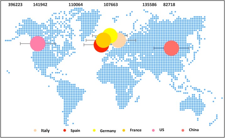
According to the World Health Organization (WHO), "COVID-19 is a disease caused by a new Coronavirus strain. The abbreviation of COVID stands for: 'CO' stands for corona, 'VI' for the virus, and 'D' for the disease. This disease was formally referred to as '2019 novel coronavirus' or '2019-nCoV.' The COVID-19 virus is a new virus linked to the same family of viruses as Severe Acute Respiratory Syndrome (SARS) and some types of a common cold." It shows symptoms similar to the flu (Influenza). The symptoms can be fever, cough, shortness of breath, pneumonia, or breathing difficulties (Unicef et al., 2020). It is a highly infectious disease which can be transmitted through person-to-person contact and through direct contact with respiratory droplets generated when an infected person coughs or sneezes (Safety and Businesses, 2020). The disease was first identified at the Wuhan city of China's Hubei province on December 29, 2019 (Li et al., 2020a). Since then, it became unstoppable and spread all over the world gradually. When the article was writing, it was confirmed that 214 countries and territories worldwide had been affected (Countries where Coronavirus has spread - Worldometer, 2021). The World Health Organization alarmed an emergency of global health issues for this COVID-19 as the confirmed cases in china raised to 76,288 on February 21, 2020 (Li et al., 2020b). About 5,790,103 people were infected worldwide by May 27, 2020, whereas the number of deaths was 357,432, and the number of recoveries was 2,497,618 (Alazab et al., 2020). Worldwide, Governments are trying to mitigate the situation by imposing lockdown, social distancing, sanitizing, work from home, international travel ban, and so forth. However, people are getting infected, and many countries are often facing difficulties in controlling the situation. The worldwide economy has seen a downfall after World War 2. Despite many actions, governments are facing difficulties to mitigate the situation. The World bank report forecasted a 5.2 % contraction in global GDP in 2020 (The Global Economic Outlook During the COVID-19 Pandemic: A Changed World, 2020). Countries like Italy, France, the United States of America, India, Spain, and Germany's confirmed cases number were rising so fast. In the Fig. 1 the top countries around the world, considering the confirmed number of COVID-19 cases have been showed with the actual number of the COVID-19 patients number which has given in the top of the figure.
Fig. 1.
Top Six Countries COVID-19 Confirmed Cases.
At the beginning, the morbidity mortality rates of COVID-19 were not predictable, especially for young children and senior-aged people (Fong et al., 2020). The mean age of these patients who died in this COVID-19 virus was 81 in Italy, and also, these patients had cardiovascular diseases, diabetes, or cancer, or smoking habits in their history record (Remuzzi and Remuzzi, 2020). This virus expanses by the contact of the affected human, mostly via small droplets generated during coughing, sneezing, or talking (Coronavirus disease, 2019 - Wikipedia, 2019). It has uncertain timing in the initial stage, and people had very little knowledge about COVID-19 characteristics.
In this situation, many epidemiological models help determine the dynamics of transmission and strategies and determine these models where some assumption parameters are required. Most of the analyses used hypothetical parameters, yet the accuracy of forecasting the future cases of COVID-19 was not so well. In this study, authors tried to predicted the cases from April 7, 2020 to July 7, 2020 using time series analysis. Time series analysis depends on only one variable, and its accuracy is also very up to the mark. The objective was to predict the covid-19 confirmed cases scenario with an approximate numerical range from April 7, 2020 to July 7, 2020. It also aimed to formulate a model that would be suitable and ideal for predicting the COVID-19 situation. This study focused on three months ahead of the forecast of the confirmed cases of COVID-19 using the ARIMA Model. This model was based on the time series analysis data from January 22, 2020, to April 7, 2020, taken from WHO (World Health Organization) (Contreras et al., 2003). These data were reliable and helped to predict an accurate forecast of the confirmed cases.
The first COVID-19 outbreak was landed in China, and gradually it is spreading in Italy, France, Germany, and the United States of America. The analysis's practical intent is to determine the time and magnitude of the epidemic peak, i.e., the maximum number of confirmed individuals cases, and gauge the effects of drastic containment measures based on simple quantitative models (Fanelli and Piazza, 2020). The national leaders and local health authorities also proposed a few prediction models to predict what will happen in the next certain days and weeks (Remuzzi and Remuzzi, 2020). Another author suggested that decision-making or predicting in a developing epidemic, where data availability is very little, may lead to high uncertainty. It is considered that data mining methodology has three main objectives - the adopted forecasting model must be the most competitive compared to its peers, the wining model should be optimized at maximum performance, and the wining model should have flexibility with other relevant time-series for multiple regression (Fong et al., 2020). The three phenomenological short-term forecasts models have been used for 5, 10, and 15 days ahead forecasts for several infectious diseases, including SARS, Ebola, pandemic influenza, and dengue (Roosa et al., 2020).
Some Authors applied the exponential smoothing family to forecast the confirmed cases of COVID-19 (Petropoulos and Makridakis, 2020). Exponential smoothing family is handy in capturing a variety of trend and seasonal forecasting patterns and combinations. The prediction range was from February 1, 2020, to March 21, 2020. However, the prediction was very close to actual cases from February 11, 2020, to March 1, 2020. (Zhan et al., 2020) predicted COVID-19 spreading profiles Susceptible Exposed-Infected-Removed (SEIR) model. However, this study was limited to South Korea, Italy, and Iran. (Chae et al., 2020) considered a susceptible, infectible, quarantined, and confirmed the recovered (SIQRK) model, which included only known data for active cases and recovered cases.
Also, other Authors predicted the COVID-19 outbreak of Saudi Arabia considering a total of 49,176 infected patients, and the data were collected from March 2, 2020, to May 15, 2020 (Alboaneen et al., 2020). Both Logistic Growth Model and Susceptible-Infected-Recovered Model was used. The models showed different results, and the authors concluded that both models had some limitations. (Vaishya et al., 2020) explored the applications of artificial intelligence for the COVID-19 pandemic, where they mentioned seven significant applications, and one of them was the projection of cases and mortality. They noted that artificial intelligence (AI) can track and forecast the virus's nature and identify the positive cases and death prediction, where it shows the most vulnerable regions, people, and countries and can take preventive measures.
In recent years, multiple methods are being used in prediction for a specific time interval. Machine learning models, empirical models, and remote sensing approaches are ubiquitous in them. However, machine learning models are the most promising methods to predict forecast with their high accuracy, which is most commonly applied in artificial neural networks (ANN), e.g., multilayer perceptron neural networks, evolutionary ANN, generalized regression neural networks (GRNN), and backpropagation neural networks (Feng et al., 2020). The other machine learning method widely used for its high accuracy for the small dataset is named the ARIMA model. Commodity prices and time series analysis have already been done with Auto-Regressive Integrated Moving Average (ARIMA) model as oil, natural gas, and electric power. The ARIMA techniques have been used for their excellent forecasting results. Also, the Auto-Regressive (AR) model was imposed on Spain and the United States confirmed cases to predict the future and had a good result (Contreras et al., 2003). Nevertheless, in this study, the ARIMA Model in predicting COVID 19 confirmed cases was the right approach to provide data results and accuracy.
2. Methods
In this study, the ARIMA time series analysis model was applied for the prediction. The Autoregressive Integrated Moving Average (ARIMA) model predicts an assumed variable's future value with several past observations and random errors with a linear function (Ömer Faruk, 2010). The ARIMA processes are a combination of some stochastic processes used to analyze time series. To perform the time series in the ARIMA model, firstly the raw data should be ready and ran some tests with the data, such as the Dickey-Fuller test, to determine the trend and find the rolling statistics of the dataset.
In this section, our proposed ARIMA model descriptions are presented with some general statistical methodology. The general scheme is as follows:
Step 1: A class of models was formulated assuming certain hypotheses.
Step 2: The model parameters were estimated.
Step 3: Check the hypotheses of the model validation. If it satisfies the conditions, go to step 4; otherwise, go to step 1 to refine the model.
Step 4: The model was ready for forecasting.
These steps were described briefly below.
Step 1:
In this step, a general ARIMA formulation was selected to model the confirmed case data. This selection was carried out by careful inspection of the main characteristics of the daily confirmed case series. In this time series analysis, high frequency, nonconstant mean and variance, and multiple seasonality (similar to daily, weekly, and periodicity) were also considered.
Step 2:
After formulating the functions of the model, the parameters of these functions must be estimated. Good estimators of the parameters were computed by assuming the data are observations of a stationary time series done by step 1 and by maximizing the likelihood concerning the parameters.
Step 3:
In step 3, a diagnosis check was used to validate the model assumptions of step 1. This calculation checked if the hypotheses made on the residuals were true. Residuals should satisfy with zero mean, constant variance, uncorrelated process, and normal distribution.
Step 4:
After that, the model was ready for the prediction. Now, go to step 2 and drive down to predict future values of confirmed cases. For this requirement, many difficulties arisen since the forecast lead time was more extensive.
3. Modeling predictions
Time Series Analysis was done for the prediction, where some components of the analysis needed to consider for our model prediction.
3.1. Components of time series
Most of the time series have trend, seasonality, and irregularity associated with them. Moreover, some of these do have a cyclic order also. However, it is not compulsory to have a pattern in the time series model. So, let us discuss each one of them in detail. These components help find suitable forecasting methods for the short term analysis (Chujai et al., 2013).
3.1.1. Trend
The Trend is a movement of higher values and lower values over a long time. So, when the values are directing upward in a time series is known as an upward trend. Also, the trend exhibits lower patterns to the downward is known as downward trends. Moreover, if it does not show any trend, it will be called a horizontal or stationary trend.
3.1.2. Seasonality
Seasonality generally has upward or downward swings. Nevertheless, it is quite a different form of a trend that shows a repeated pattern for a fixed period.
3.1.3. Irregularity
Irregularity is also known as noise. It is the iritic nature of data and is also called residual. So, it happens for only a short duration and not repeated like the other.
3.1.4. Cyclic
Cyclic is the repeating up and down movement of a set of data in a graph. It means it can happen over more than a year and have no fixed pattern. They can repeat in one year, two years, or half of a year, and it is harder to predict.
For predicting a time series analysis, it is crucial to consider the stationarity of the dataset. Time series requires data to be stationary, and it is a must for the analysis. The stationary has three components: the constant mean, constant variance, and autocovariance that does not depend on time. To check whether the dataset is stationary or not, two popular tests exist in python. The one is the rolling statistics and the Augmented Dickey-Fuller test (ADCF).
3.2. ARIMA model
ARIMA is one of the best models for time series data, which the combination of two models. The AR Model stands for the Auto Regressive part, and the MA model stands for the Moving Average part. These two models are bound together by the integration part, indicated by" I" in the ARIMA Model. The ARIMA model has three parameters: "P" is the autoregressive lags, "Q" is the moving average, and "d" is the order of differentiation.
For predicting our dataset in the ARIMA model, firstly found the rolling statistics of the dataset. Then the Dickey-Fuller test was performed and estimated the trends of the dataset. Again, the Dickey-Fuller test was performed associated with the trends. Then the Auto Correlation graph (ACF) and Partial Auto Correlation graph (PACF) were performed to determine the value of Q and P. After that, the AR model and the MA model were performed, and it predicted the future. Finally, we converted the dataset into the cumulative sum and plotted the graph.
4. Forecast future
4.1. Data
We obtained the daily basis data of the confirmed cases worldwide from the World Health Organization (WHO) website (Novel Coronavirus (COVID-19) Cases Data - Humanitarian Data Exchange, 2020). The data contained over 198 countries, Covid-19 cases across the world. Data updates were collected from January 22, 2020, to April 7, 2020. The short time-series was affected by irregularities and reporting lags, so the cumulative curves were more stable and likely yield more stability and reliability estimations. So, we determined the stationary of the data set, residual of the dataset and removed the unnecessary errors from our prediction model.
4.2. Predicting procedure
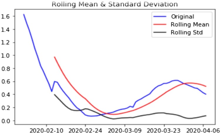
Jupyter Notebook was used for the python coding. The dataset was plotted in graph and determined the rolling statistics, and then the model performed the Augmented Dickey–Fuller test (ADF) test to determine the Test Statistic, p-value, Lags Used, and Number of Observations Used. From the graph, it has been seen the data were not stationary. After that, the model estimated the trends, which was the log of the indexed dataset. Then we found the difference between the moving average and the actual number of the cases. After that, the model performed the Augmented Dickey–Fuller test (ADF) test which showed in Fig. 2 . In the Fig. 2 the red line representing the rolling Mean, the blue line was the original dataset, and the black line was the rolling standard deviation. Here, it determinate that there were no such trends, and the Test Statistic, p-value, Critical Values also changed.
Fig. 2.
Augmented Dickey–Fuller test (ADF) test result.
Then the model determined the trend of the time series, and it was an upward trend time series. Also, there was another transformation where the model determined the difference between dataset Log Scale and Moving Exponential Decay Average, and the stationarity level was checked. Here again the Test Statistic, p-value, Critical Values were changed.
Then again the values were shifted into a time series. Again, the stationary test of the data set was performed. And this time also there was no trend present, and it was relatively flat.
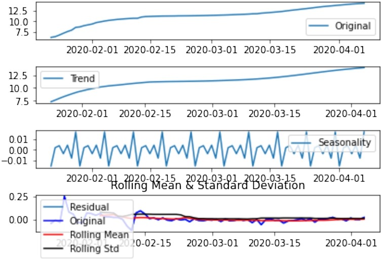
After that, the Trend, Seasonal, and residual graph were found from the dataset. Fig. 3 visualized the original dataset graph, the trend of the dataset, seasonality, and residual graph, which was the irregularity presented in the data set. Then, the residual and tested result found as stationary and visualized that the data were not stationary, and the value of "d" was determined.
Fig. 3.
Trend, Seasonal and Residual graph of the dataset.
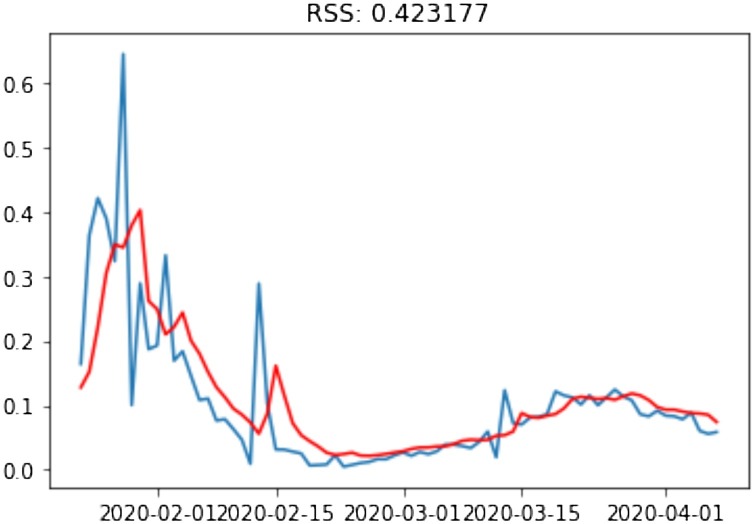
After that, to calculate the "p-value," the data needed to plot the ACF graph, and for the "Q-value," the model need to performed the PACF graph. The model then calculated the Residual Sum of Squares (RSS) value for the AR model from these values. Fig. 4 showed that the value of RSS was 0.423177, which was satisfactory.
Fig. 4.
RSS Value of the AR Model.
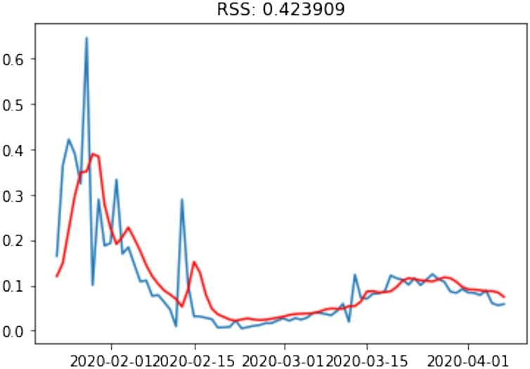
Moreover, from these values, the RSS value for the MA model was calculated. From Fig. 5 , the value of RSS was 0.423909 found, which was also excellent.
Fig. 5.
RSS Value of the MA Model.
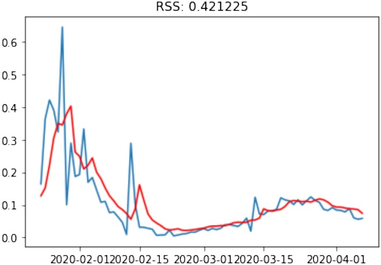
In the Autoregressive part, the RSS was 0.405828 found and concerning the moving average part, the RSS was 0.421225, and it combined with both of them and calculated the RSS of the ARIMA Model. From Fig. 6 , it was visualized the RSS of the ARIMA model was 0.405828, which was a good result.
Fig. 6.
RSS Value of the ARIMA Model.
Then the fitting values from our ARIMA model analysis was calculated. Then the model converted the fitted values into the series format. So, the model determined the dates over the predictions and transferred our predicted data into our original format.
For prediction, there was a function called predict in python, which helped us predict the number of confirmed COVID-19 cases from April 7, 2020 to July 7, 2020.
5. Result
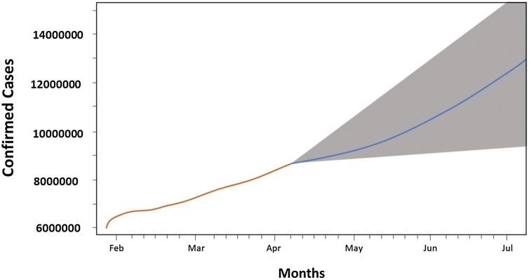
At first, the model determined the data point. As the model prepared for visualize three months' prediction, the data point was 90 by using the plot.predict function. Over here, in the Fig. 7 it has showed that the blue line is the forecasted value and the gray part is the confidence level. Now, however, this forecasting was done yet this value never existed at the confidence level. So, from April 7, 2020, to July 7, 2020, the prediction was like this.
Fig. 7.
Forecast of next three months (April 7, 2020–July 7, 2020).
6. Discussion
In this study, authors provided a short time forecast of the possible cumulative number of the COVID-19 confirmed cases of this epidemic globally. As this epidemic is worldwide, authors published three months ahead of forecast in the ARIMA model. Based on the data model up until April 7, 2020, authors forecasted a cumulative number of confirmed cases from April 7, 2020, to July 7, 2020, in the year of 2020 was between 9,189,262 – 14,906,483 worldwide. The result showed that the accuracies of prediction and, subsequently, multiple-step forecasting were high. The confidence level of this prediction was about 95 %, which was satisfactory for the prediction. Our experience revealed that forecasting improved when the training time was longer. From the model it was observed that the prediction intervals' width decreased on average as more data were included for forecasts. However, if the data were reliable, and there would be no second transmission, the ARIMA model predicted that the COVID-19 outbreak might have the same number of confirmed cases globally.
7. Conclusion and future work
The study explored COVID-19 growth rate closely and predicted the number of confirmed cases and aimed to let the world know what the situation would look like. Authors found that the curve of the COVID-19 confirmed cases would go upward, which called on the world to be more conscious about this virus. In conclusion, our most recent forecasts, based on data, remain relatively stable. ARIMA model predicted that what stage the epidemic could have been reached around the world. This likely reflected the impact of the broad spectrum of this epidemic. The forecast was based on the assumption that current mitigation efforts would continue. Many research works have been done for short terms forecasting period like 5, 10 and 15 days. Where in this study, authors took data of last three months and predicted the scenario of next three months. If the data set is large, then it can predict long time period with precision as well. Moreover, the ARIMA model showed excellent accuracy in the time series analysis prediction which previous models could not achieve.
So, this model should be applied for predicting future analysis of any dataset. The limitations that observed during the prediction was comparatively small dataset and the prediction was based on a pandemic where the variation in the data set was high. If there were more extensive and less variance dataset, then the output would be more accurate. In future, researcher can explore some prediction models such as an artificial neural network (ANN), Bayesian networks, and Support Vector Machines (SVM) in COVID-19. This model is also applicable in future pandemics and to predict any type of disease affected patients.
Authorship contributions
Category 1
Conception and design of study: Chyon Fuad Ahmed, Suman Md. Nazmul Hasan acquisition of data: Chyon Fuad Ahmed analysis and/or interpretation of data: Chyon Fuad Ahmed, Suman Md. Nazmul Hasan.
Category 2
Drafting the manuscript: Fahim Md. Rafiul Islam, Suman Md. Nazmul Hasan revising the manuscript critically for important intellectual content: Ahmmed Md. Sazol, Chyon Fuad Ahmed.
Category 3
Approval of the version of the manuscript to be published (the names of all authors must be listed): Chyon Fuad Ahmed, Suman Md. Nazmul Hasan, Fahim Md. Rafiul Islam, Ahmmed Md. Sazol.
Declaration of Competing Interest
The authors declare that they have no known competing financial interests or personal relationships that could have appeared to influence the work reported in this paper.
Data availability
Data will be made available on request.
References
- Alazab M., et al. COVID-19 prediction and detection using deep learning. Int. J. Comput. Inf. Syst. Ind. Manage. Appl. 2020;12(April):168–181. [Google Scholar]
- Alboaneen D., et al. Predicting the epidemiological outbreak of the coronavirus disease 2019 (COVID-19) in Saudi Arabia. Int. J. Environ. Res. Public Health. 2020;17(12):1–10. doi: 10.3390/ijerph17124568. [DOI] [PMC free article] [PubMed] [Google Scholar]
- Chae S.Y., et al. Estimation of infection rate and predictions of disease spreading based on initial individuals infected with COVID-19. Front. Phys. 2020;8(August):1–6. doi: 10.3389/fphy.2020.00311. [DOI] [Google Scholar]
- Chujai P., Kerdprasop N., Kerdprasop K. Vol. 2202. 2013. Time series analysis of household electric consumption with ARIMA and ARMA models; pp. 295–300. (Lecture Notes in Engineering and Computer Science). [Google Scholar]
- Contreras J., et al. ARIMA models to predict next-day electricity prices. IEEE Trans. Power Syst. 2003;18(3):1014–1020. doi: 10.1109/TPWRS.2002.804943. [DOI] [Google Scholar]
- Coronavirus disease 2019 - Wikipedia (2019). Available at: https://en.wikipedia.org/wiki/Coronavirus_disease_2019#cite_note-CDCTrans-16 (Accessed: 10 April 2020).
- Countries where Coronavirus has spread - Worldometer (no date). Available at: https://www.worldometers.info/coronavirus/countries-where-coronavirus-has-spread/ (Accessed: 18 November 2020).
- Fanelli D., Piazza F. Analysis and forecast of COVID-19 spreading in China, Italy and France’. Chaos Solitons Fractals. 2020;134:109761. doi: 10.1016/j.chaos.2020.109761. Elsevier Ltd. [DOI] [PMC free article] [PubMed] [Google Scholar]
- Feng Y., et al. Machine learning models to quantify and map daily global solar radiation and photovoltaic power. Renew. Sustain. Energy Rev. 2020;118(May 2019):109393. doi: 10.1016/j.rser.2019.109393. Elsevier Ltd. [DOI] [Google Scholar]
- Fong S.J., et al. Finding an accurate early forecasting model from small dataset: a case of 2019-nCoV novel coronavirus outbreak. Int. J. Interact. Multimed. Artif. Intell. 2020;6(1):132. doi: 10.9781/ijimai.2020.02.002. [DOI] [Google Scholar]
- Li Q., et al. Early transmission dynamics in Wuhan, China, of novel coronavirus–Infected pneumonia. N. Engl. J. Med. 2020;382(13):1199–1207. doi: 10.1056/nejmoa2001316. [DOI] [PMC free article] [PubMed] [Google Scholar]
- Li X., et al. Evolutionary history, potential intermediate animal host, and cross-species analyses of SARS-CoV-2. J. Med. Virol. 2020;92(6):602–611. doi: 10.1002/jmv.25731. [DOI] [PMC free article] [PubMed] [Google Scholar]
- Novel Coronavirus (COVID-19) Cases Data - Humanitarian Data Exchange (2020). Available at: https://data.humdata.org/dataset/novel-coronavirus-2019-ncov-cases (Accessed: 11 April 2020).
- Ömer Faruk D. A hybrid neural network and ARIMA model for water quality time series prediction. Eng. Appl. Artif. Intell. 2010;23(4):586–594. doi: 10.1016/j.engappai.2009.09.015. [DOI] [Google Scholar]
- Petropoulos F., Makridakis S. Forecasting the novel coronavirus COVID-19. PLoS One. 2020;15(3):1–8. doi: 10.1371/journal.pone.0231236. [DOI] [PMC free article] [PubMed] [Google Scholar]
- Remuzzi A., Remuzzi G. COVID-19 and Italy: what next? Lancet. 2020;2:10–13. doi: 10.1016/S0140-6736(20)30627-9. Elsevier Ltd. [DOI] [PMC free article] [PubMed] [Google Scholar]
- Roosa K., et al. Real-time forecasts of the COVID-19 epidemic in China from February 5th to February 24th, 2020. Infect. Dis. Model. 2020;5:256–263. doi: 10.1016/j.idm.2020.02.002. Elsevier Ltd. [DOI] [PMC free article] [PubMed] [Google Scholar]
- Safety F., Businesses F. COVID-19 and Food Safety: Guidance for Food Businesses: Interim Guidance. 2020. COVID-19 and food safety: guidance for food businesses: interim guidance; pp. 1–6. (April) [DOI] [Google Scholar]
- The Global Economic Outlook During the COVID-19 Pandemic: A Changed World (2020). Available at: https://www.worldbank.org/en/news/feature/2020/06/08/the-global-economic-outlook-during-the-covid-19-pandemic-a-changed-world (Accessed: 23 November 2020).
- Unicef, WHO, IFRC . Key Messages and Actions for COVID-19 Prevention and Control in Schools. 2020. Key messages and actions for prevention and control in schools. (March), p. 13. Available at: https://www.who.int/docs/default-source/coronaviruse/key-messages-and-actions-for-covid-19-prevention-and-control-in-schools-march-2020.pdf?sfvrsn=baf81d52_4#:∼:text=COVID-19isa,2019-nCoV. [Google Scholar]
- Vaishya R., et al. Artificial Intelligence (AI) applications for COVID-19 pandemic. Diabetes Metab. Syndr. Clin. Res. Rev. 2020;14(4):337–339. doi: 10.1016/j.dsx.2020.04.012. [DOI] [PMC free article] [PubMed] [Google Scholar]
- Zhan C., et al. Prediction of COVID-19 spreading profiles in South Korea, Italy and Iran by data-driven coding. PLoS One. 2020;15(7 July):1–17. doi: 10.1371/journal.pone.0234763. [DOI] [PMC free article] [PubMed] [Google Scholar]
Associated Data
This section collects any data citations, data availability statements, or supplementary materials included in this article.
Data Availability Statement
Data will be made available on request.


