An analysis of contact tracing protocol in an over-dispersed SEIQR Covid-like disease

Abstract

The aim of this work is to study an over-dispersed SEIQR infectious disease and obtain optimal methods of contact tracing. A prototypical example of such a disease is that of the current SARS-CoV-2 pandemic. In consequence, this study is immediately applicable to the current health crisis. In this paper, we introduce both a discrete and continuous model for various modes of contact tracing. From the continuous model, we derive a basic reproductive number and study the stability of the equilibrium points. We also implement the continuous and discrete models numerically and further analyze the effectiveness of different types of contact tracing and their cost on society. Additionally, through these simulations, we also study the effect that various parameters of the disease have on its evolution.

1. Introduction

The global health crisis brought about by SARS-CoV-2 has revealed our lack of preparedness to deal with a pandemic. As of today, 7 months since the WHO declared the coronavirus a global pandemic, there have been 112,000,000 detected infections of COVID19 and 2,500,000 detected deaths [1] and there is still no unified protocol for contact tracing or collection of data. Due to the unreliability and heterogeneities of the collection of data, in this paper, we look to use only the already well-established characteristics of COVID19 to study optimal control efforts. These methods of disease prevention will in turn apply to any disease with a similar structure and qualities to COVID19.

There are several well-established methods of infectious disease control such as physical distancing, disinfection of hands and surfaces, and vaccination. In this article, we will focus on contact tracing and how it should be carried out to reduce the spread of over-dispersed infectious diseases. Possible ways to improve contact tracing have recently been the object of study of a growing number of researchers. Tedelay the authors conclude via an agent-based model that the delay between the onset of symptoms and the positive diagnosis is critical to containing the advance of COVID19. In [2], [3] the writers conclude that bidirectional contact tracing is superior to traditional contact tracing. However, to the extent of our knowledge, and at the time of publication, this result has only been shown using agent-based models or simple approximations of the spread of COVID19 whereas in this work we propose a continuous model, as well as a discrete one, to verify this hypothesis. In addition, we estimate the cost of each contact tracing protocol in terms of the number of individuals that enter quarantine.

The mathematical study of the propagation of biological agents plays a fundamental role when it comes to understanding the behavior of infectious diseases. Furthermore, mathematical models help us to both determine (in a theoretical way) and evaluate control measures. Modern mathematical epidemiology goes back to Kermack and McKendrick model [4]. This is a very simple SIR (Susceptible–Infectious–Recovered) compartmental model where the dynamics are modeled in terms of a system of ordinary differential equations. Since then, several models based on this paradigm have been proposed in the scientific literature (see, for example, [5], [6], and references therein). Of special interest are those works devoted to the study and analysis the basic reproductive number [7], [8]. During the last two years, the research in this field has increased notably due to the social impact of the COVID19 pandemic [9], [10], [11]

To achieve this aim our work is organized as follows: in Section 2 we introduce the two main ways of contact tracing that are currently used and the negative binomial distribution, which will serve as an over-dispersed offspring distribution. In Sections 3, 4 we build a continuous model for an $SEIQR$ disease based on each of the two types of contact tracing introduced in the first section. We will take COVID19 as the prototype for our study as it fits the SEIQR model and is a prototypical example of an over-dispersed disease. In Section 5 we study the stability of the equilibrium points to these models and calculate their basic reproductive number ${\mathcal{R}}_0$. In Section 6 we conduct various numerical simulations to study the previously discussed continuous models. We then construct in Section 7 a discrete (stochastic) version of our continuous models, conduct further simulations and analyze the obtained results. Finally, in Section 8 we discuss the conclusions that one may obtain from our study and propose further avenues of research.

2. Contact tracing protocol and offspring distribution

In this section, we introduce the two types of contact tracing that we will discuss throughout our work. To effectively complete this study we also introduce the binomial distribution, which will be used as the offspring distribution of our over-dispersed disease.

2.1. Forward contact tracing and backward contact tracing

The two contact tracing models that will be studied in this work are the following:

Forwards contact tracing (FCT).

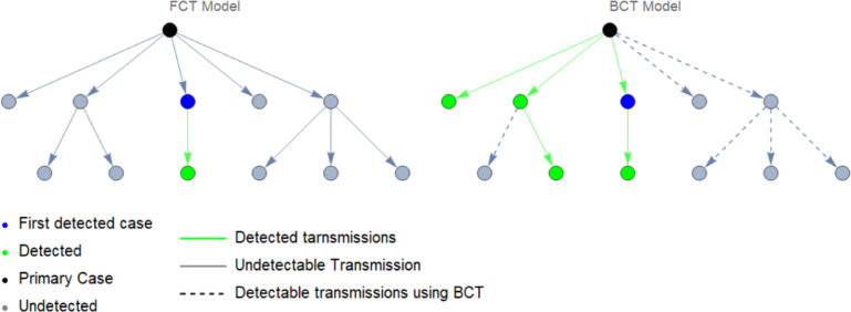
Under this contact tracing protocol, once an infected individual is detected said individual is placed in quarantine and an attempt is made to find all people the infected individual had a potentially dangerous contact with since contracting the disease. The idea behind this method is to eliminate any potential infections resulting from the infected individual. This is the contact tracing that has been used in many countries in response to COVID19 [12]. In the particular case of COVID19, one attempts to locate all close contacts that occurred two days back from symptom onset [13].

Backwards contact tracing (BCT).

With this protocol, once an infected individual is detected said individual is placed in quarantine one attempts to locate the person that first infected the subject (the primary case). Once this is achieved all individuals that had dangerous contact with the primary case are placed in quarantine. This method is designed for diseases that spread mostly through large clusters (super-spreader events). The reasoning behind BCT protocol is that an individual who is detected to be infected was likely infected by a primary case that caused more infections than the detected individual themselves (this is similar to the so-called friendship paradox). Thus, the optimal way to react would be to locate the primary infection and quarantine everyone that they may have infected.

Below, in Fig. 1, is a graph showing an example of both BCT and FCT protocol. Some cases, though in theory detectable, remain undiscovered due to human implementation which is inherently imperfect.

Fig. 1.

Comparison of FCT (left) and BCT (right) contact tracing protocol.

When carrying out BCT one uses, in addition to the same tests as FCT, some additional tests to find the primary case. In principle, this may seem like it would lead to more testing, which could prove to be an issue if testing capacity is limited. However, if BCT is more effective, it may end up controlling the disease earlier than a FCT protocol. Due to this BCT may lead to even fewer tests overall than FCT.

2.2. The binomial distribution and a discussion of dispersion

Diseases like the flu spread in a linear and predictable way where the reproductive number ${\mathcal{R}}_0$ encapsulates almost all the information of the disease. In essence, the assumption that each infected individual will results in exactly ${\mathcal{R}}_0$ secondary infections is a good one.

On the other hand, as current data shows [14], [15], [16], COVID19 is a representative case of an overly dispersed disease. That is, the distribution of secondary cases caused by an infected individual has a much higher variance and the disease spreads through large clusters of secondary infections. This has important consequences for effective disease control measures.

The offspring distribution of a disease is the distribution that assigns a probability $p_n$ to the event $E_n=\left\{\text{the cluster has }n\text{infected individuals}\right\}$. It is often useful when considering the offspring distribution $X$ of an overly dispersed disease to assume that $X$ follows a negative binomial distribution [17]. We now introduce this distribution:

The negative binomial distribution with parameters $k\in {\mathbb{R}}^{+}$, and $0<p<1$ is the distribution $X$ with values in $\mathbb{N}$ such that

$$\mathbb{P}(X=n)=\frac{\Gamma (n+k)}{\Gamma \left(k\right)n!}{p}^k{(1-p)}^n\forall n\in \mathbb{N},$$ (1)

where $\Gamma$ is the gamma function. We symbolize that $X$ follows a negative binomial distribution by $X\sim NB(k,p)$. By manipulating the series that define the mean and variance of $X$ one may show that the mean and the variance of a random variable following binomial distribution $X\sim NB(k,p)$ are respectively

$$\mu ≔E\left[X\right]=\frac{pk}{1-p};{\sigma }^2≔Var\left[X\right]=\frac{pk}{{(1-p)}^2}.$$ (2)

We deduce by solving the system of equations in (2) for ${\sigma }^2$ that the variance of $X$ is a quadratic function of its mean with

$${\sigma }^2=\mu +\frac{{\mu }^2}{k}.$$ (3)

The terms ${\mu }^2/k,k$ are respectively called the over-dispersion and dispersion parameter of $x$ and indicate an over-dispersion of our distribution with respect to the Poisson distribution. To observe this consider the Poisson distribution of mean $\mu$, $Poisson\left(\mu \right)$. Then $Poisson\left(\mu \right)$ also has variance equal to $\mu$ and it holds that, if we maintain $\mu$ fixed, the limit as the over-dispersion goes to zero of $X$ is $Poisson\left(\mu \right)$. That is:

$$NB(k,\mu /(k+\mu ))\stackrel{k\to \infty }{⟶}Poisson\left(\mu \right),$$ (4)

where the above convergence is in distribution and can be obtained in the usual fashion by considering the limit of the probabilities $p_n≔\mathbb{P}(X=n)$. For all this, the negative binomial distribution is useful when considering infectious diseases whose offspring distribution has a high variance. In particular, in [15] it was found that the negative binomial distribution was the distribution that best fit the data for the offspring distribution of COVID19.

3. A continuous forward contact tracing model

In this section, we will analyze the dynamics of COVID19 in a population which uses as a control measure forward contact tracing (see Section 2.1).

We begin with a heuristic discussion of the equations that govern our model. It is crucial to realize that any model is only as strong as the set of assumptions that it makes. For this reason, we will carefully lay out all the hypotheses made and explain how they lead logically to each term in the equations that follow. In this way, we hope that the reader may gain full insight into the workings of the models to come, and thus, may be able to adjust them to new data and information that arises and even to other diseases with similar epidemiological properties.

3.1. The compartments

The mathematical model introduced in this work is compartmental where the population is subdivided into five compartments corresponding to susceptible, exposed, infected, quarantined, and recovered individuals. Specifically, a SEIQR model is considered where the dynamics consist of the following process: susceptible individuals become exposed when they have been successfully infected; exposed individuals become infectious once the latency period finishes; susceptible, exposed and infectious individuals can be quarantined; and infectious individuals can recover from infection when the infectious period finishes. Specifically, our model will be made up of the following compartments:

• •Susceptible ($S$): These are the members of the population that are at risk of contracting the disease. On becoming infected these individuals pass to compartment $E$.
• •Exposed ($E$): Individuals that have been infected by the disease but still have not had time to develop clinical symptoms. Nonetheless, the current consensus is that members of $E$ are still infectious and may be the cause of a substantial portion of COVID19 infections [18]. On finishing the incubating phase these individuals pass to compartment $I_a$ or $I_s$.
• •Infectious asymptomatic ($I_a$): Infectious individuals that do not develop clinical symptoms during their infectious period.
• •Infectious symptomatic ($I_s$): Infectious individuals that develop clinical symptoms during their infectious period.
• •Quarantined susceptible ($Q_S$): Susceptible individuals that are in quarantine due to close contact with confirmed positive cases. Members of this compartment cannot become infected and thus remain in $Q_S$ until their quarantine period ends.
• •Recovered ($R$): Infectious individuals that, are either in quarantine and will remain there till they are no longer infectious, or have already completed their infectious phase and are no longer infectious. Individuals that enter this compartment remain in it forever and contribute to no further infections. Thus we do not allow for reinfections as, though in the real world reinfection remains possible, it is exceedingly rare [19].

3.2. Deduction of the state equations and some hypotheses

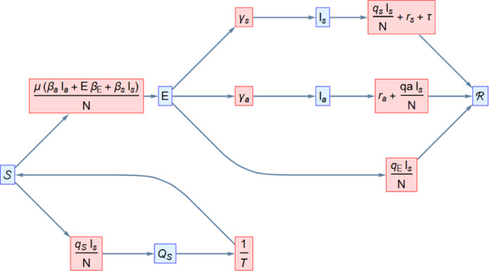
The dynamics of the forward contact tracing model are illustrated in Fig. 2. The equations we will be working with are

$$S^{\prime }=\frac{1}{T}{Q}_S-\mu \left(\frac{q_S}{\mu }{I}_s+{\beta }_{E}E+{\beta }_s{I}_s+{\beta }_a{I}_a\right)\frac{S}{N},$$ (5)

$$E^{\prime }=\mu \left({\beta }_{E}E+{\beta }_s{I}_s+{\beta }_a{I}_a\right)\frac{S}{N}-{\gamma }_{E}E-q_E{I}_s\frac{E}{N},$$ (6)

$$I_s^{\prime }={\gamma }_{s}E-(r_s+\tau )I_s-q_s\frac{I_s^2}{N},$$ (7)

$$I_a^{\prime }={\gamma }_{a}E-r_a{I}_a-q_a{I}_s\frac{I_a}{N},$$ (8)

$$Q_S^{\prime }=q_s{I}_s\frac{S}{N}-\frac{1}{T}{Q}_S,$$ (9)

$$R^{\prime }=(r_s+\tau )I_s+r_a{I}_a+\left(q_{E}E+q_s{I}_s+q_a{I}_a\right)\frac{I_s}{N},$$ (10)

$$(S,E,I_s,I_a,Q_S,R)\left(0\right)=(S_0,E_0,I_{s,0},I_{a,0},Q_{S,0},R_0),$$ (11)

where, for brevity in the expression, we have omitted the time $t$ at which the functions $S,E,I_s,I_a,Q_s,R$ are valued (all other terms are constants, i.e. independent of time). This said we now proceed to explain the above equations, clarifying each term in said equations and mentioning the assumptions used to arrive at them. We begin by mentioning that we assume the natural mortality and birth rate to be zero as, due to the short time frame during which the epidemic has taken place, these parameters should not qualitatively affect our model.

Fig. 2.

Flow diagram associated with the FCT compartmental model.

3.3. Glossary of parameters

In what follows we will describe the epidemiological coefficients involved in the proposed model.

• •Let $N$ be the total amount of individuals in the population.
• •Set $T$ the average time in days that a susceptible individual remains in quarantine.
• •Consider $\mu ≔E\left[X\right]={\sum }_{n}n{p}_n$ where $p_n$ is the probability that a cluster caused by an infectious individual results in $n$ infections amongst a totally susceptible population. That is $p_n=\mathbb{P}(X=n)$ where $X$ is the offspring distribution.
• •Suppose that ${\beta }_E,{\beta }_s,{\beta }_a$ are the rate of clusters caused by one individual of group $E,I_s,I_a$ respectively in an entirely susceptible population.
• •Assume that $q_S,q_E,q_s,q_a$ are the expected rate of dangerous contacts that result in quarantine per member of $I_s$ amongst a population made out entirely of members of $S,E,I_s,I_a$ respectively. The reason why these parameters are not supposed identical is that we allow in theory for different contact rates amongst the separate compartments.
• •Set ${\gamma }_s,{\gamma }_a$ the rates at which a member of $E$ move to $I_s,I_a$ respectively and in consequence ${\gamma }_E≔{\gamma }_s+{\gamma }_a$ is the rate at which a member of $E$ moves to either $I_s$ or $I_a$.
• •Let $r_s,r_a$ be the rates of recovery of individuals in $I_s,I_a$ respectively.
• •$\tau$ is the self-quarantine rate of symptomatic individuals due to awareness of their symptoms.
• •${\tilde{r}}_s≔r_s+\tau$ is the sum of $r_s,\tau$ and indicates the rate at which individuals leave compartment $I_s$ due to recovery/quarantine.

3.4. An explanation of the state equations

(1) Susceptible individuals that become infected per unit time.

We have that ${\beta }_{E}E$ is the number of clusters caused by exposed individuals per unit time. Therefore, $p_n{\beta }_{E}E$ is the number of clusters we expect to cause $n$ infections in an entirely susceptible population per unit time. In consequence, the sum of the terms $n{p}_n{\beta }_{E}ES/N$ is the number of infections we expect to be caused by exposed individuals per unit time. A similar discussion goes through for clusters caused by $I_a,I_s$ with which we arrive at the infinite sum in (5).

(2) Susceptible individuals that enter quarantine per unit time.

Though in reality susceptible individuals enter quarantine due to close contact with any individual in $E,I_s,I_a$ who has become detected, due to the great majority of detected cases being due to symptomatic individuals [20] we consider for simplicity that the rate at which susceptible individuals enter quarantine is proportional only to the product $I_{s}S$ (that is without considering the products $I_{a}S$ or $ES$). Note that this approximation is additionally bolstered by the fact that the amount of symptomatic individuals $I_s$ is predictive of the number of individuals in $E,I_a$. Thus we set the number of susceptible individuals entering quarantine per unit time to $q_S{I}_{s}S/N$. We also employ similar reasoning to set the next three terms.

(3) Exposed that enter quarantine per unit time.

$q_{E}E{I}_s/N$. This term is analogous to the previous term in (2) where now we need only replace $q_S$ by the quarantine coefficient $q_E$ for exposed individuals.

(4) Infectious symptomatic that quarantine/recover per unit time.

$q_s{I}_s^2/N+(r_s+\tau )I_s$. Once again, we have a term that indicates quarantine due to close contact with detected symptomatic individuals. In this case this term is $q_s{I}_s^2/N$. Furthermore, we have the additional summands $r_s{I}_s$, $\tau I_s$ due to recovery and self detection.

(5) Infectious asymptomatic that quarantine/recover per unit time.

$q_a{I}_s{I}_a/N+r_a{I}_a$. Once more, we have a term due to close contact with detected susceptible individuals and which in this case is $q_a{I}_s{I}_a/N$ and a term $r_a{I}_a$ due to recovery of members of $I_a$.

(6) Susceptible individuals that leave quarantine per unit time.

Due to the definition of the parameters this is $Q_S/T$. Current guidelines are to quarantine for 14 days in the case of close contact with an infectious individual [21]. For this reason, we will set $T=14$ throughout the remainder of our work.

(7) Individuals that become exposed per unit time.

By definition of $E$ and $S$ this is the same as the number of susceptible individuals that become infected per unit time (term (1)).

(8) Individuals that become $I_a$ or $I_s$ per unit time.

This is equal to ${\gamma }_{E}E$; where ${\gamma }_{s}E$ individuals go to compartment $I_s$ and ${\gamma }_{a}E$ of them go to compartment $I_a$.

(9) Individuals that recover per unit time.

This is equal to $r_s{I}_s+r_a{I}_a$; where the amount preceding from $I_s,I_a$ are $r_s{I}_s,r_a{I}_a$ respectively.

(10) Infectious individuals that enter quarantine.

This is equal to (3)+(4)+(5). As previously explained these individuals go to compartment $R$ on entering quarantine.

3.5. A continuous forward contact tracing model with vaccination

For completeness we note that it is also possible to consider in the above model the inclusion of a vaccine. One approach to doing so would be to, as in [22]: set a vaccination rate and efficacy ${\xi }_v$ and ${\epsilon }_v$ respectively and to split the susceptible population into two groups; those that have been vaccinated ($S_v$) and those that are yet unvaccinated ($S_u$). We would also have to subdivide the compartment $Q_S$ into two compartment $Q_v$, and $Q_u$, corresponding to the population of $S_v,S_u$ respectively that have entered quarantine. The analogous of the model in Eqs. (5)–(10) would now be:

$$S_u^{\prime }=\frac{1}{T}{Q}_u-\mu \left(\frac{q_S}{\mu }{I}_s+{\beta }_{E}E+{\beta }_s{I}_s+{\beta }_a{I}_a\right)\frac{S_u}{N}-{\xi }_v{S}_u,$$ (12)

$$S_v^{\prime }=\frac{1}{T}{Q}_v-(1-{\epsilon }_v)\mu (q_S{I}_s+{\beta }_{E}E+{\beta }_s{I}_s+{\beta }_a{I}_a)\frac{S_v}{N},$$ (13)

$$E^{\prime }=\mu ({\beta }_{E}E+{\beta }_s{I}_s+{\beta }_a{I}_a)\frac{S_u}{N}+(1-{\epsilon }_v)\mu (q_S{I}_s+{\beta }_{E}E+{\beta }_s{I}_s+{\beta }_a{I}_a)\frac{S_v}{N}-{\gamma }_{E}E-q_E{I}_s\frac{E}{N},$$ (14)

$$I_s^{\prime }={\gamma }_{s}E-(r_s+\tau )I_s-q_s\frac{I_s^2}{N},$$ (15)

$$I_a^{\prime }={\gamma }_{a}E-r_a{I}_a-q_a{I}_s\frac{I_a}{N},$$ (16)

$$Q_u^{\prime }=q_s{I}_s\frac{S_u}{N}-\frac{1}{T}{Q}_u,$$ (17)

$$Q_v^{\prime }=q_v{I}_v\frac{S_v}{N}-\frac{1}{T}{Q}_v,$$ (18)

$$R^{\prime }=(r_s+\tau )I_s+r_a{I}_a+(q_{E}E+q_s{I}_s+q_a{I}_a)\frac{I_s}{N},$$ (19)

$$(S_u,S_v,E,I_s,I_a,Q_u,Q_v,R)\left(0\right)=(S_{u,0},S_{v,0},E_0,I_{s,0},I_{a,0},Q_{u,0},Q_{v,0},R_0).$$ (20)

However, since our main intent is to study the usage of contact tracing at the beginning of an infectious outbreak we will not use the above model in what remains of our work.

4. A continuous backward contact tracing model

In this section, we introduce a similar continuous compartmental model for COVID19 which now incorporates backward contact tracing.

As was previously discussed backward contact tracing is especially advantageous when the offspring distribution $X$ has high variance. It is important to notice that, in the FCT model of Section 3, the only characteristic of the offspring distribution that appears is its mean $\mu$ (which appears in the term of susceptible individuals that become infected per unit time in Eqs. (5), (6)). In the FCT model, no other properties of the offspring distribution are used for quarantine purposes. That is, we are disregarding extra important information, namely the over-dispersion of $X$.

On the other hand, as we shall soon see, the variance and hence the dispersion of the offspring distribution will become important in our BCT model. The only terms that we need to change when considering BCT protocol are the terms involving individuals that enter quarantine. We reason as follows: consider the event $D$ an infectious individual was detected, as before, let $E_n$ stand for “the detected individual forms part of a cluster of $n$ infected individuals” and set $p_n≔\mathbb{P}\left(E_n\right)$. Then, since ${\left\{E_n\right\}}_{n=1}^{\infty }$ partitions the sample space of possible clusters we have that, by Bayes Theorem:

$$\mathbb{P}\left(E_n\right|D)=\frac{\mathbb{P}\left(D\right|E_n)p_n}{\sum _{j=0}^{\infty }\mathbb{P}\left(E_j\right)\mathbb{P}\left(D\right|E_j)}.$$ (21)

If we now make the reasonable supposition that the detection of an infected person in a cluster is proportional to the number of people in said cluster, i.e. 

$$\mathbb{P}\left(D\right|E_j)=j\mathbb{P}\left(D\right|E_1).$$ (22)

We obtain that

$$\mathbb{P}\left(E_n\right|D)=\frac{n{p}_n\mathbb{P}\left(D\right|E_1)}{\sum _{j=0}^{\infty }j\mathbb{P}\left(E_j\right)\mathbb{P}\left(D\right|E_1)}=\frac{n{p}_n}{E\left[X\right]}.$$ (23)

In consequence, once we detect an infected individual, the average amount of infections we detect from the original cluster is (assuming we detect all dangerous contacts):

$$\sum _{n=0}^{\infty }n\mathbb{P}\left(E_n\right|D)=\sum _{n=0}^{\infty }\frac{n^2{p}_n}{E\left[X\right]}=\frac{Var\left[X\right]+E{\left[X\right]}^2}{E\left[X\right]}=\frac{{\sigma }^2+{\mu }^2}{\mu }=\frac{{\sigma }^2}{\mu }+\mu .$$ (24)

. In the case that $X\sim NB(k,p)$ and adding the average forward detection $\mu$ we obtain from Eqs. (2), (3) that we can write:

$$\text{Detected infections from }D=\left(\sum _{n=0}^{\infty }n\mathbb{P}\left(E_n\right|D)\right)+\mu =\left(1+\frac{\mu }{k}+\mu \right)+\mu .$$ (25)

Where the first term corresponds to those detected backwards and the second to those tested forwards.

By once again simplifying and considering that individuals quarantine only due to contacts with symptomatic individuals we obtain that the quarantine term (10) of the previous model may be rewritten as:

(26)

Note that the division by $\mu$ is due to our previous terminology in which $\mu$ infections lead to $q_S,q_E,q_s,q_a$ among the respective populations. Where the ${\tilde{q}}_E,{\tilde{q}}_s,{\tilde{q}}_a$ have the same meaning as previously. That is, they reflect the ratio of dangerous contacts and the imperfections of the testing and tracing process (the latter now being different, reason for which these terms are also different, as it may be more difficult to trace contacts that occur farther back in time). Similar reasoning allows us to set the term of susceptible individuals entering quarantine per unit time to:

(27)

To simplify our notation we define

(28)

By defining also ${\hat{q}}_E,{\hat{q}}_s,{\hat{q}}_a$ in a similar fashion we have that our backward contact tracing model is

$$S^{\prime }=\frac{1}{T}{Q}_S-\mu \left(\frac{{\hat{q}}_S}{\mu }{I}_s+{\beta }_{E}E+{\beta }_s{I}_s+{\beta }_a{I}_a\right)\frac{S}{N},$$ (29)

$$E^{\prime }=\mu ({\beta }_{E}E+{\beta }_s{I}_s+{\beta }_a{I}_a)\frac{S}{N}-{\gamma }_{E}E-{\hat{q}}_E{I}_s\frac{E}{N},$$ (30)

$$I_s^{\prime }={\gamma }_{s}E-(r_s+\tau )I_s-{\hat{q}}_s\frac{I_s^2}{N},$$ (31)

$$I_a^{\prime }={\gamma }_{a}E-r_a{I}_a-{\hat{q}}_a{I}_s\frac{I_a}{N},$$ (32)

$$Q_S^{\prime }={\hat{q}}_S{I}_s\frac{S}{N}-\frac{Q_S}{T},$$ (33)

$$R^{\prime }=(r_s+\tau )I_s+r_a{I}_a+({\hat{q}}_{E}E+{\hat{q}}_s{I}_s+{\hat{q}}_a{I}_a)\frac{I_s}{N},$$ (34)

$$(S,E,I_s,I_a,Q_S,R)\left(0\right)=(S_0,E_0,I_{s,0},I_{a,0},Q_{S,0},R_0).$$ (35)

Note that it is clearly qualitatively of the same type as our forwards contact tracing model with the only difference being that the quarantine coefficients ${\hat{q}}_S,{\hat{q}}_E,{\hat{q}}_s,{\hat{q}}_a$ are larger. In an identical fashion to Section 3.5, it is also possible to consider the case where there exists a vaccination process.

5. Stability and reproductive number

In this section, we find the equilibrium points and basic reproductive number for the models of the preceding section. We also study the stability of said equilibrium points.

We first study the stability points of our continuous FCT model comprised of Eqs. (5) to (10). We suppose that all parameters for this model are strictly positive (see the glossary of parameters in Section 3.3) and we restrict our attention to the biologically feasible domain ${\mathbb{R}}_{+}^6$, which is invariant under solutions to our equations in Sections 3.2 and 4.

A verification shows that the only equilibrium points are disease-free and contain only members in $S,R$. Furthermore, since the total population $N$ of our model is constant (as can be checked by adding together all the state equations to obtain $N^{\prime }=0$) the only equilibrium points of our model are the elements of

$$\mathcal{P}=\{(S,E,I_s,I_a,Q_S,R)=(S_0,0,0,0,0,N-S_0):0\le S_0\le N\}\subset {\mathbb{R}}_{+}^6,$$ (36)

Note that $\mathcal{P}$ is formed by all points of the state set at which everyone in the population is susceptible or has recovered (or, equivalently, system states at which no one is infected or in quarantine).

We have that the linear approximation of our system at such a point has the form

$$\left(\begin{array}{cccccc}\hfill 0\hfill & \hfill -\frac{S_0}{N}\mu {\beta }_E\hfill & \hfill -\frac{S_0}{N}(\mu {\beta }_s+q_S)\hfill & \hfill -\frac{S_0}{N}{\beta }_a\hfill & \hfill \frac{1}{T}\hfill & \hfill 0\hfill \\ \hfill 0\hfill & \hfill \frac{S_0}{N}\mu {\beta }_E-{\gamma }_E\hfill & \hfill \frac{S_0}{N}\mu {\beta }_s\hfill & \hfill \frac{S_0}{N}\mu {\beta }_a\hfill & \hfill 0\hfill & \hfill 0\hfill \\ \hfill 0\hfill & \hfill {\gamma }_s\hfill & \hfill -{\tilde{r}}_s\hfill & \hfill 0\hfill & \hfill 0\hfill & \hfill 0\hfill \\ \hfill 0\hfill & \hfill {\gamma }_a\hfill & \hfill 0\hfill & \hfill -r_a\hfill & \hfill 0\hfill & \hfill 0\hfill \\ \hfill 0\hfill & \hfill 0\hfill & \hfill \frac{S_0}{N}{q}_S\hfill & \hfill 0\hfill & \hfill -\frac{1}{T}\hfill & \hfill 0\hfill \\ \hfill 0\hfill & \hfill 0\hfill & \hfill {\tilde{r}}_s\hfill & \hfill r_a\hfill & \hfill 0\hfill & \hfill 0\hfill \end{array}\right).$$ (37)

As we can see by the box formed by the columns and rows $2,3,4$ of the matrix (37), which correspond to the infected individuals $E,I_s$ and $I_a$ respectively, the new infection matrix $F$ and the transition matrix $V$ are given by

$$F=\frac{S_0}{N}\mu \left(\begin{array}{ccc}\hfill {\beta }_E\hfill & \hfill {\beta }_s\hfill & \hfill {\beta }_a\hfill \\ \hfill 0\hfill & \hfill 0\hfill & \hfill 0\hfill \\ \hfill 0\hfill & \hfill 0\hfill & \hfill 0\hfill \end{array}\right);V=\left(\begin{array}{ccc}\hfill {\gamma }_E\hfill & \hfill 0\hfill & \hfill 0\hfill \\ \hfill -{\gamma }_s\hfill & \hfill {\tilde{r}}_s\hfill & \hfill 0\hfill \\ \hfill -{\gamma }_a\hfill & \hfill 0\hfill & \hfill r_a\hfill \end{array}\right).$$ (38)

The basic reproductive number ${\mathcal{R}}_0$ is defined as the spectral radius of $F{V}^{-1}$ (see for example [23]). From (38) we obtain that

$$F{V}^{-1}=\frac{S_0}{N}\mu \left(\begin{array}{ccc}\hfill \frac{1}{{\gamma }_E}\left({\beta }_E+\frac{{\gamma }_s}{{\tilde{r}}_s}{\beta }_s+\frac{{\gamma }_a}{r_a}{\beta }_a\right)\hfill & \hfill \frac{{\beta }_s}{{\tilde{r}}_s}\hfill & \hfill \frac{{\beta }_a}{r_a}\hfill \\ \hfill 0\hfill & \hfill 0\hfill & \hfill 0\hfill \\ \hfill 0\hfill & \hfill 0\hfill & \hfill 0\hfill \end{array}\right),$$ (39)

thus we obtain that $F{V}^{-1}$ has as its unique non-zero eigenvalue the first entry of the above matrix, i.e. we obtain an ${\mathcal{R}}_0$ of

$${\mathcal{R}}_0≔\rho \left(F{V}^{-1}\right)=\frac{\mu S_0}{{\gamma }_{E}N}\left({\beta }_E+\frac{{\gamma }_s}{{\tilde{r}}_s}{\beta }_s+\frac{{\gamma }_a}{r_a}{\beta }_a\right)≔\frac{S_0}{N}(R_E+R_s+R_a)$$ (40)

This expression just obtained for ${\mathcal{R}}_0$ is very intuitive in that it provides the relative importance of each infectious compartment $E,I_a,I_s$ to our disease. Due to the meaning of each parameter, we have that:

• •The term $R_E$ measures the average infections one expects from an individual in compartment $E$ during its period ${\gamma }_E^{-1}$ in said compartment.
• •$R_s$ measures the number of infections one expects from an individual in compartment $I_s$ during their symptomatic period ${\tilde{r}}_s^{-1}$ and weighted by the relative occurrence of symptomatic infections with respect to the total of symptomatic and non-symptomatic infections, ${\gamma }_s/{\gamma }_E$.
• •$R_a$ is completely analogous to $R_s$ where the above heuristics now apply to compartment $I_a$ instead of $I_s$.

Due to all this, we have that $R_E+R_s+R_a$ represent the reproduction number of our disease of a completely susceptible population. By weighting this sum by the proportion of susceptible individuals in our population, $S_0/N$, we obtain our reproductive number in (40). This final weighting represents that in the hypothesis of our model we have taken the effectiveness of infection to be inversely proportional to $S_0/N$.

In terms of stability of the equilibrium points, we have that the characteristic polynomial of the linearized system in (37) is of the form $P\left(x\right)=x^{2}Q\left(x\right)$, where $Q\left(x\right)$ is another polynomial. Thus $P\left(x\right)$ has zero as two of its roots and we cannot directly conclude the stability of our equilibrium points. Nonetheless, the following result holds

Theorem 5.1

The equilibrium points$\mathcal{P}$of the system of Eqs. (5) are locally asymptotically stable if ${\mathcal{R}}_0<1$ and unstable if ${\mathcal{R}}_0>1$ .

Proof

Let $\mathcal{F}:{\mathbb{R}}_{+}^6\to {\mathbb{R}}^6$ denote the rate of appearance of new infections. That is, if we use the shorthand $x≔(S,E,I_s,I_a,Q,R)$, then

$$\mathcal{F}\left(x\right)≔\left(0,\mu \left({\beta }_{E}E+{\beta }_s{I}_s+{\beta }_a{I}_a\right)\frac{S}{N},0,0,0,0\right).$$ (41)

Furthermore let ${\mathcal{V}}^{+},{\mathcal{V}}^{-}:{\mathbb{R}}_{+}^6\to {\mathbb{R}}^6$, be the rate of transfer of individuals in and out of each compartment by all other means. That is

$${\mathcal{V}}^{+}\left(x\right)=\left(\frac{Q_S}{T},0,{\gamma }_{s}E,{\gamma }_{a}E,q_S{I}_s\frac{S}{N},r_a{I}_a+\widetilde{r_S}{I}_s+(q_{E}E+q_s{I}_s+q_a{I}_a)\frac{I_s}{N}\right),$$ (42)

$${\mathcal{V}}^{-}\left(x\right)=\left(q_S{I}_s\frac{S}{N},{\gamma }_{E}E+q_{E}E\frac{I_s}{N},{\tilde{r}}_s{I}_s+q_s\frac{I_s^2}{N},r_a{I}_a+q_a{I}_s\frac{I_a}{N},\frac{Q_S}{T},0\right).$$ (43)

Then $\mathcal{F},{\mathcal{V}}^{+},{\mathcal{V}}^{-}$ verify the conditions $\left(A1\right)-\left(A5\right)$ of article [24] (conditions $\left(A1\right)-\left(A4\right)$ are immediate and $\left(A5\right)$ may be verified via a calculation) and hence, we may apply Theorem 2 of this same article to conclude that our Theorem 5.1 holds. □

The analogous study of the continuous BCT model is practically identical. This is because, as we already mentioned, the system is qualitatively the same. The only difference is that the BCT’s quarantine coefficients ${\hat{q}}_E,{\hat{q}}_s,{\hat{q}}_a$ are larger than the FCT’s quarantine coefficients $q_E,q_s,q_a$. In particular, we obtain the same equilibrium points, stability, and ${\mathcal{R}}_0$ for this model.

6. Numerical simulation of the continuous FCT and BCT model

In this section, we simulate the state equations obtained in Section 3.2 and Section 4 for forward and backward contact tracing protocol respectively. We conduct all simulations with Mathematica.

One of our continuous simulations will be conducted with $N=4.7\cdot 10^7$ individuals to be representative of the population of Spain. The other continuous simulation will use $N=1000$ individuals so as to be more comparable with a discrete implementation developed in later sections. This difference in initial population between the continuous simulations may lead one to hypothesize that the existence of finite size effects makes results between the two incomparable. However, this is not the case due to a nice scale invariance of the solutions to our models.

Theorem 6.1 Scale invariance —

Let $X\left(t\right)=(S,E,I_s,I_a,Q_S,R)\left(t\right)$ be a solution to (5) – (10) with initial data and population respectively

$$X_0=(S_0,E_0,I_{s,0},I_{a,0},Q_{S,0},R_0);N=S_0+E_0+I_{s,0}+I_{a,0}+Q_{S,0}+R_0.$$

Then $\lambda X\left(t\right)$ is solution to (5) – (10) with initial data and population respectively

$$\lambda X_0;\lambda N.$$

An identical result holds for solutions to (29) – (34)

Proof

The proof is a simple substitution of the components of $\lambda X$ into Eqs. (5)–(10) and a usage of the linearity of the derivative. □

We first obtain a numerical simulation to said state equations with the following parameters:

• •$N=1000$ is the population such that we take 10 people to be initially exposed.
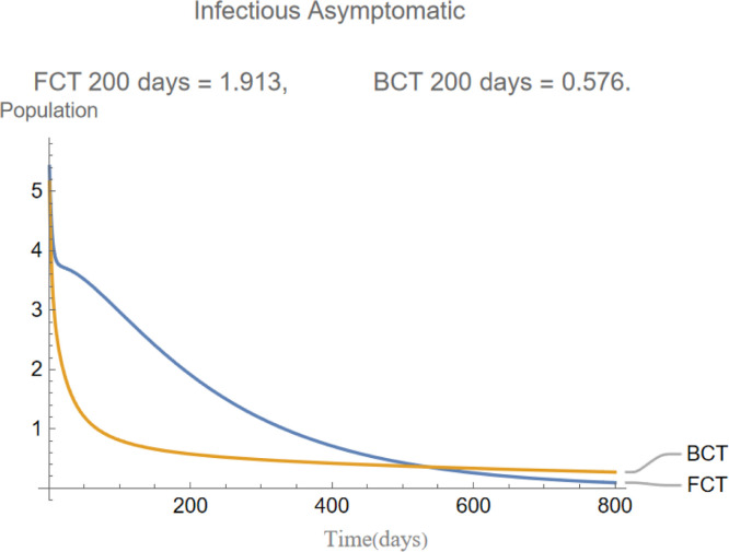
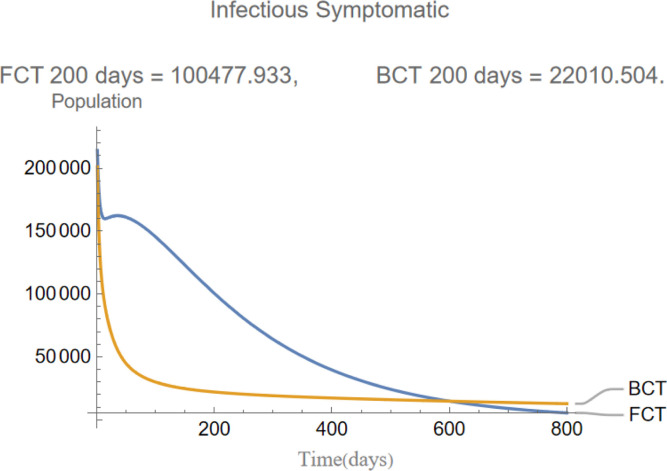
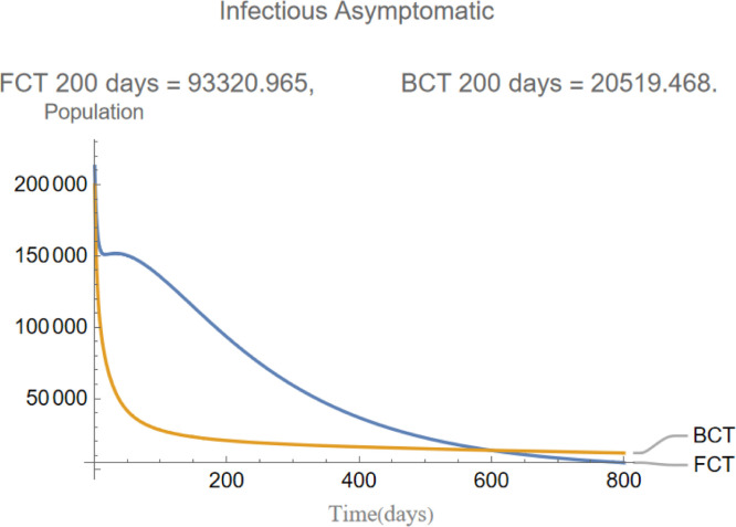
• •${\gamma }_s={\gamma }_a=\frac{1}{10}$ indicates that the incubation period of the disease is $5$ days and that infections are equally distributed between asymptomatic and symptomatic. This will in turn cause the evolution of these two compartments to be almost identical as it is shown later in Fig. 5, Fig. 6.
• •$q_S=q_E=q_s=q_a=2$ indicate that we expect to find $2$ close contacts per symptomatic infection in a wholly susceptible population and likewise for an entirely exposed, asymptomatic, symptomatic population.
• •$\tau =0.3/14$ indicates that we expect that 30% of symptomatic individuals will self-quarantine throughout their infectious period.
• •${\beta }_E=1/14,{\beta }_s=3/14,{\beta }_a=4/14$ indicates that we expect individuals in $E,I_s,I_a$ to cause $1,3,4$ infectious clusters respectively in a 14 day time span.
• •$\mu =0.4,k=0.96$ indicates that we expect the offspring distribution of each cluster to follow a negative binomial distribution with mean 0.4 and dispersion 0.96.
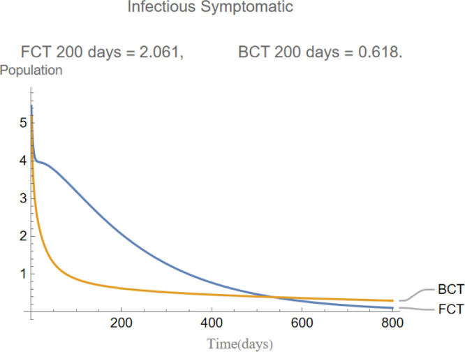
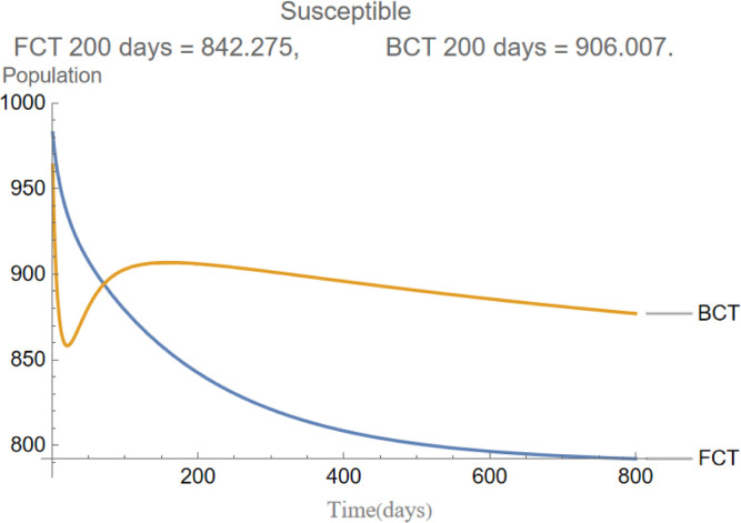
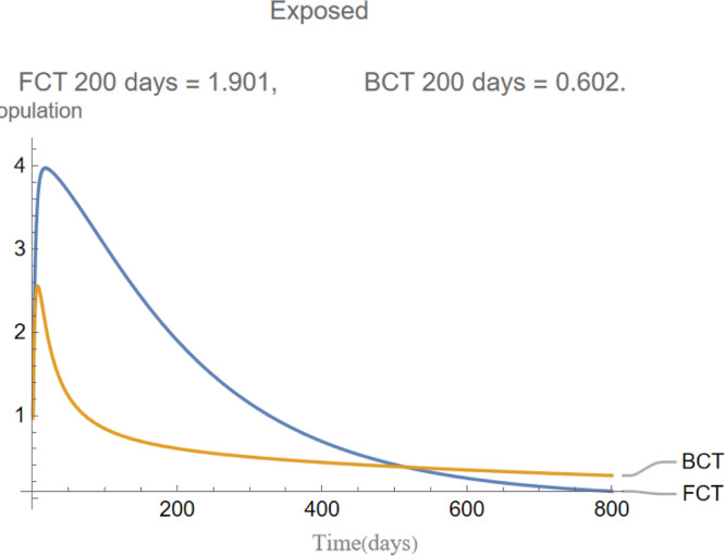
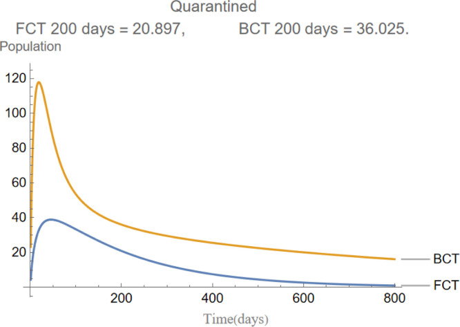
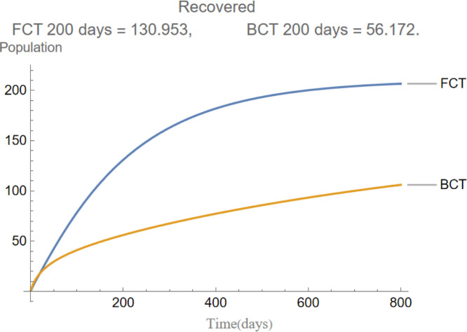
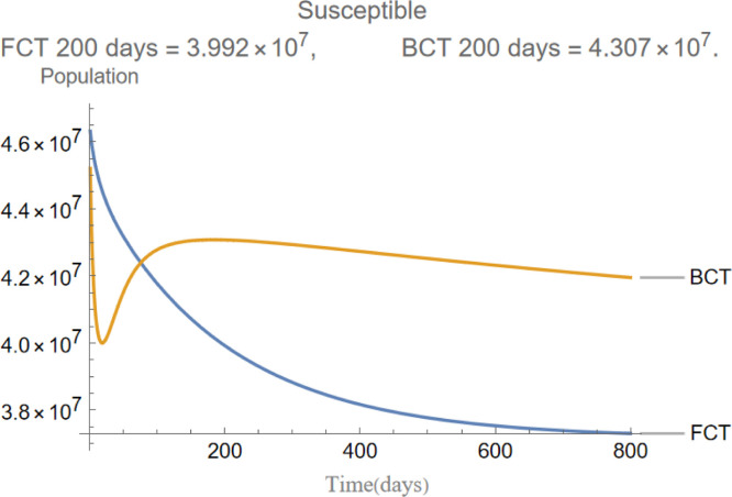
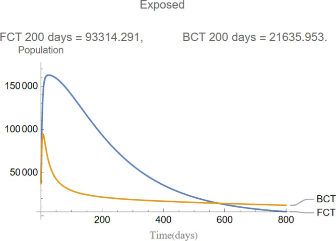
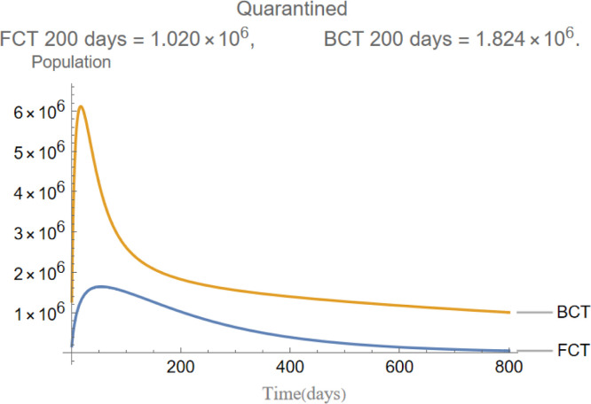
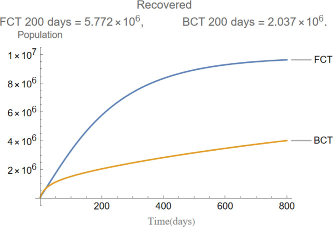
• •$r_a=1/10,r_s=1/14$ are the infectious frequency of $I_s,I_a$ and correspond to an infectious period of 14, 10 days respectively. Fig. 3, Fig. 4, Fig. 5, Fig. 6, Fig. 7, Fig. 8 illustrate respectively the evolution of compartments $S,E,I_s,I_a$, $Q$ and $R$ in a simulation for the above values of the parameters. Above each graph are the number of individuals in each compartment after 200 days for each mode of contact tracing. We see that, as we already expected (as the quarantine coefficients for the BCT model are higher than those of the FCT model), the BCT protocol (blue) performed better than the FCT protocol (red). After 200 days for example, as can be seen by adding together the number of people in $E,I_a,I_s,R$, gives that the number of people infected after 200 days is 137,58 for FCT, BCT respectively. That is BCT performs 58% better than FCT after 200 days. Which is hardly negligible. It is important to keep in mind that, the best way of measuring the performance of each protocol is not by how counting how many infected individuals there are at the end of the simulation, but by how many are infected throughout. In the below simulations, we have for example that on day 800 there are 0.28 infectives (members of $E,I_s$ or $I_a$) in the FCT model and 0.84 in the BCT model. By this metric the FCT model would perform better, however, this difference is very small when one considers that, after this same number of days, 100 more individuals have been infected under FCT protocol than BCT (206 as compared to 106).

Fig. 5.

The evolution of infectious symptomatic individuals.

Fig. 6.

The evolution of infectious asymptomatic individuals.

Fig. 3.

The evolution of susceptible individuals.

Fig. 4.

The evolution of exposed individuals.

Fig. 7.

The evolution of quarantined individuals.

Fig. 8.

The evolution of recovered individuals.

Let us perform another simulation we now take an even more over-dispersed disease and hence a smaller $k$ which we set $k=0.3$ as has been estimated for COVID19 [15]. We also take $N=4.7\cdot 10^7$ and set 1% of the initial population to be infected, keeping all other parameters identical. Fig. 9, Fig. 10, Fig. 11, Fig. 12, Fig. 13, Fig. 14 show the evolution of compartments $S,E,I_s,I_a,Q$, and $R$ respectively in a simulation for the above values of the parameters. Once again, above each graph, we include the number of individuals in each compartment after 200 days for each mode of contact tracing. As we can see, we now obtain an even more appreciable difference. Namely, we have that after $200$ days a total of $6.1\cdot 10^6,2.1\cdot 10^6$ individuals have been infected for the FCT and BCT respectively. In other words, the BCT model performs 66% better than its counterpart. On the $800$th day we have that $9.6\cdot 10^6,2.1\cdot 4.1^6$ individuals are infected for the FCT and BCT respectively. This corresponds to a 57% reduction in infections by using BCT versus FCT protocol.

Fig. 9.

The evolution of susceptible individuals.

Fig. 10.

The evolution of exposed individuals.

Fig. 11.

The evolution of infectious symptomatic individuals.

Fig. 12.

The evolution of infectious asymptomatic individuals.

Fig. 13.

The evolution of quarantined individuals.

Fig. 14.

The evolution of recovered individuals.

7. A discrete implementation

Here we implement four stochastic discrete models for a highly dispersed disease. Firstly we discuss a model with no quarantine, secondly a model with FCT protocol, thirdly a model with an intermediate BCT and fourthly a model with a “complete BCT” in the lines of what was discussed earlier.

7.1. Shared properties: setup and outbreaks

The discussion in this section is shared for all discrete models. Firstly, the connections between the individuals of our population are modeled by a scale-free network (characterized by a node-degree distribution of power-law form and independence of connectivity scale) [25] following the Barabá si-Albert algorithm with $N=1000$ nodes and at least $m=5$ connections from each node. We also start with a fixed amount of individuals in each compartment given by $S_0,E_0,I_{a,0},I_{s,0},Q_{S,0}$, and $R_0$. We also fix periods of time $T_E,T_a,T_s$ that individuals spend in the infectious compartments $E,I_a$ and $I_s$ respectively. Our model advances in discrete time steps of $1$ day and in each step determines the outbreaks and infections that occur as follows:

(1) Determination of an outbreak.

An infected individual $v$ in group $E$ produces an outbreak with probability

$$f_E\left(v\right)≔\frac{r_S\left(v\right)}{r\left(v\right)}{p}_E$$ (44)

where $p_E$ is a previously fixed number between $0$ and $1$ that reflects the probability of an outbreak amongst an entirely susceptible population and where $r_S\left(v\right),r\left(v\right)$ are the amount of susceptible and total individuals within a distance of $2$ from $v$. Where, by distance we between two nodes, we mean the length of the shortest path in the graph between these two nodes. In this way, we ponder the frequency of an outbreak stemming from $v$ by the frequency of the nearby susceptible population. In an analogous fashion, we define $f_s$ and $f_a$ as the probability of an outbreak occurring due to an infectious asymptomatic and symptomatic individual respectively by

$$f_a\left(v\right)≔\frac{r_S\left(v\right)}{r\left(v\right)}{p}_a,f_E\left(v\right)≔\frac{r_S\left(v\right)}{r\left(v\right)}{p}_s,$$ (45)

where $p_s,p_a$ now determine the probability of an outbreak amongst an entirely susceptible population by a symptomatic, asymptomatic individual respectively.

(2) Determination of infections.

If $v$ causes an outbreak it infects a number of individuals following an offspring distribution $X$ given by the negative binomial distribution $NB(k,p)$. First infecting those at distance one and then, if necessary (if $X$ took a value larger than the susceptible population within a distance of $1$ from $V$), infecting those at a distance of $2$ or less from $v$. If $X$ is even larger than $r_S\left(v\right)$ than the extra infections are disregarded. It is worth noting that in the simulations carried out $r_2\left(v\right)$ was typically around 15% of the total population and such events were extremely rare.

(3) Transition between states.

• 1.Susceptible to exposed: Susceptible individuals infected by an outbreak (see point (2)) move to compartment $E$.
• 2.Exposed to infected: After an individual $v$ spends $T_E$ days (time steps) in compartment $E$ they move to compartment $I_s,I_a$ with probability ${\gamma }_s/{\gamma }_E,{\gamma }_a/{\gamma }_E$ respectively.
• 3.Recovery: Individuals of $I_s,I_a$ that have spent $T_s,T_a$ days in their respective compartments $I_s,I_a$ move to compartment $R$.
• 4.
  Quarantining:

  • (a)
    Model with no quarantine: No such process occurs.
  • (b)
    Model with FCT protocol: Each time step each individual $v$ in compartment $I_s$ has a probability $\tau$ of self-quarantining and thus moving to compartment $R$. If this event occurs then each neighbor at a distance of $1$ from $v$ becomes detected and placed in quarantine with probability $p_d$. This detection occurs instantly. In terms of compartments these individuals move to $Q_S$ if they were susceptible and to $R$ otherwise. Note that none of these detections trigger an additional round of detections, as we do not continue testing backwards.
  • (c)
    Model with “intermediate” BCT protocol: As before, each time step each individual $v_0$ in compartment $I_s$ has a probability $\tau$ of self-quarantining and thus moving to compartment $R$. If this event occurs then each neighbor at a distance of $1$ from $v$ instantly becomes detected with probability $p_d$. We then test these individuals with a test of sensitivity $s$. If any node tests positive then each of its untested neighbors becomes detected and placed in quarantine with a probability $p_d$. In terms of compartments these individuals move to $Q_S$ if they were susceptible and to $R$ otherwise. Note that none of these latter detections are tested or trigger an additional round of detections. In this sense, the backwards contact tracing is intermediate as we do not continue testing down the chain of infections.
  • (d)
    Model with BCT protocol Once again, each individual $v_0$ in compartment $I_s$ has a probability $\tau$ of self-quarantining and thus moving to compartment $R$. If this event occurs then we consider the set $V_1$ of neighbors at a distance of $1$ from $v$. Members of this set instantly become detected with probability $p_d$ and placed in a temporary quarantine. The next day the tests, with sensitivity $s$, for the nodes in $V_1$ are completed and those that test negative are removed from their temporary quarantine and placed back in their previous compartment. On the other hand, if a node $v_1^{+}$ tests positive it is placed in quarantine, as in the previous model. Let us set

    $$V_1^{+}=\{v_1^{+}\in V_1:v_1^{+}\text{ tests positive}\}$$ (46)

    to be the nodes of $V_1$ that tested positive and

    $$V_2=\{v_2:d(v_1^{+},v_2)=1\text{ for some }{v}_1^{+}\in V_1^{+}\}$$ (47)

    to be the nodes at a distance of $1$ from elements of $V_1^{+}$. We now continue our chain by detecting elements of $V_2$ with probability $p_d$ and testing those detected with the same type of test. This test will be completed the next day, two days from the self-quarantine of $v_0$. This process continues until one of the sets $V_n^{+}$ is empty. Note that in this case, we continue testing all the way down the (detected) chain of infections.
• 5.Quarantine to other states: In the cases where individuals were tested (BCT models) it was explained how these individuals were returned to their original compartments once a negative test was obtained. In the case where there is no testing (FCT models and some cases in intermediate BCT), these individuals return to being susceptible after a quarantine of $T$ days.

7.2. Results and discussion of a stochastic simulation

This completes the explanation of our discrete models. It is interesting to note the following. In the continuous model, to not overly complicate the resulting equations, we imposed quarantining due only to contact with members of $I_s$ (see Eqs. (9), (29)). However, in a discrete implementation, we have been able to consider quarantining that occurs also due to contact with members of $E,I_a$. This kind of quarantining occurs to different degrees in both our BCT models. For each mode of contact tracing, we simulated our discrete models 1000 times using the same parameters as in our first continuous model. Additionally, each simulation spanned two hundred days.

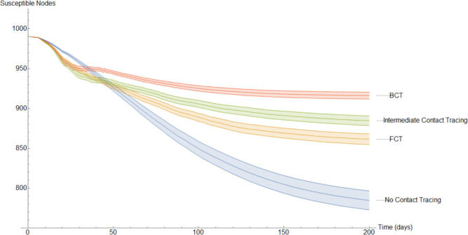
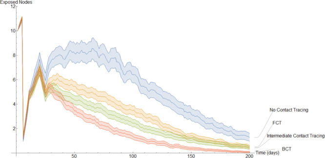
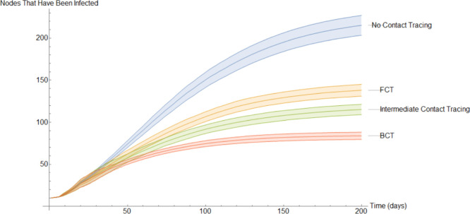
To get a better idea of how these different methods of contact tracing compare amongst each other we will study the mean of these simulations. In Fig. 15, Fig. 16, Fig. 17, Fig. 18, Fig. 19, Fig. 20, Fig. 21 we plot the mean amount of nodes in each of the models’ compartments for each one of the considered models. Additionally, we give 95% confidence intervals of said means. These confidence intervals are shown in the following graphs as bands enveloping each curve. The confidence intervals are calculated by using the Mathematica function “FindDistribution” to find a functional form to fit the distribution of the data obtained in the simulations. This distribution is then used to calculate the aforementioned confidence intervals.

Fig. 15.

Evolution of the average susceptible nodes.

Fig. 16.

Evolution of the average exposed nodes.

Fig. 17.

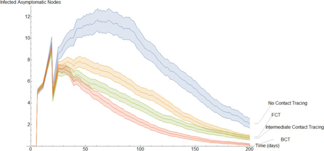
Evolution of the average infected asymptomatic nodes.

Fig. 18.

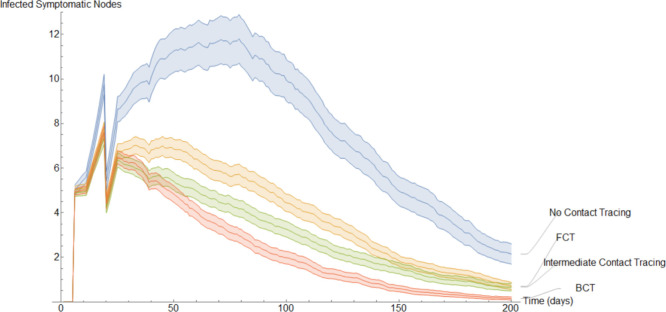
Evolution of the average infected symptomatic nodes.

Fig. 19.

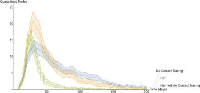
Evolution of the average infected symptomatic nodes.

Fig. 20.

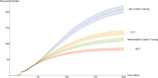
Evolution of the average recovered individuals.

Fig. 21.

Evolution of the average nodes that have been infected at some point.

In Fig. 15 the mean amount of susceptible nodes each of the 200 days of the simulations is shown. As we can see, BCT is the best performing method of contact tracing followed by the intermediate and FCT methods. Unsurprisingly, the model without quarantine was the one with the worst performance. As we will see, in Fig. 16, Fig. 17, Fig. 18, Fig. 19, Fig. 20 the same ranking is repeated. The very first few days it may seem, paradoxically, that the method without contact tracing is doing better than its fellows. However, this is simply because in the models with contact tracing a small part of the nodes that are not in the susceptible compartment are in the quarantined compartment.

Fig. 16 shows the evolution of the change in the average exposed individuals. At the start every model has 10 exposed nodes, this number increases slightly the first 5 days as these exposed nodes infect others before sharply dropping when the 10 initial exposed nodes transition into one of the infected compartments. After this initial stage, the BCT model distinguishes itself from the others as a result of its more effective quarantining process.

In Fig. 17, we show the evolution of the infected asymptomatic population. Qualitatively, it is very similar to the evolution of the exposed population. It is worth noting that the models that implement worse methods of quarantine have larger confidence intervals as they are more prone to large outbreaks.

Fig. 18 is qualitative and quantitatively almost identical to Fig. 17. This is a result of the fact that in these simulations we set an exposed individual to be equally likely to become symptomatic or asymptomatic. However, a discerning eye may note that on average there are slightly more infected asymptomatic nodes than infected symptomatic nodes. This is a result of a portion of the infected symptomatic nodes self quarantining.

One of the most impressive aspects of the model that implements BCT is the fact that the reduction of infections comes despite fewer individuals being quarantined on average. This is reflected in Fig. 19.

In Fig. 20, we show the evolution of the average recovered individuals. We remind the reader that, the larger the amount of nodes in the recovered compartment for a given model, the worse this model performs, as these are nodes that have been previously infected.

Perhaps the best way of comparing the models is by using the average nodes that have been infected at some point. This is shown in Fig. 21 which, due to the large amount of time elapsed, is very similar to Fig. 20.

The numerical values at the end of day 200 are shown in Fig. 22

Fig. 22.

Confidence interval for the nodes that have been infected at the end of 200 days.

This grid suggests that a quarantine strategy that implements BCT has a 99.9% of having between 58% to 64% fewer infections than a population that does not implement contact tracing after 200 days. Between 35% to 43% fewer infections than a population that uses FCT and between 22% to 32% fewer infections than a population that implements intermediate contact tracing.

8. Conclusions

Recent events have manifested the importance of contact tracing in controlling infectious diseases. In most cases, the predominant method used is forward contact tracing. With this strategy, once an infected individual is detected, the people with whom that person was recently in contact are warned and recommended to self-quarantine. However, as we have seen throughout this study, backward contact tracing presents notable benefits in comparison to forward contact tracing when the disease in question has a high over-dispersion. These advantages are not only theoretical but have been verified experimentally. In both our discrete and continuous models, backward contact tracing performs better than its counterpart especially when the over-dispersion is greater. This strongly suggests that backward contact tracing should be the preferred method of detection in infectious diseases that present a significant variability of the number of infections caused by an outbreak.

The implementation of backward contact tracing is likely more difficult as it is based on detecting contacts that occur further in the past than those detected through forward contact tracing. Furthermore, this adds the logistical difficulty that the number of contacts to be traced through BCT may be significantly higher than those through BCT. However, since the advantages gained through BCT are in large part due to the detection of large clusters, in practice we recommend that maximum priority is assigned to contacts occurring at events with large agglomerations of people such as those occurring at parties, concerts, sporting events or public transport. These contacts may be easier to trace as attending such as event is more difficult to forget and leverage the main principle of BCT, cluster detection. Successful examples of such an implementation have been conducted, among others, by the governments of Japan and South Korea [26], [27]. Furthermore, though it may seem that more tests are needed to conduct BCT, we showed in Section 7.2 that in fact fewer tests are needed in the long run when using BCT as compared to FCT.

In this article, we focused on the role in disease prevention of different modes of contact tracing isolated from other control methods and determined that backward contact tracing was best suited to over-dispersed diseases. A future study could use this finding to test what other control methods (such as vaccination, stay-at-home orders, social distancing, prohibition of large gatherings...) best pair with backward contact tracing while analyzing their respective cost on society. It is all but certain that sometime in the future, humanity will face another pandemic, and it is the hope of the authors that this paper can help to shed light on more effective techniques for controlling and preventing any such disease that may lie ahead.

Finally, though it was determined via the stochastic implementation of Section 7, that backward contact tracing is not only more efficient but imposes a lower cost on society than its alternatives, we did not study the number of tests performed in each mode of contact tracing. Since, at least at first, backwards contact tracing requires more tests than other modes of contact tracing, a possible further study could take this into account to determine how the availability of tests influences the relative efficiency of backward contact tracing with respect to other modes of contact tracing. In this sense, an additional analysis of the criticality of the system by means of the finite-size scaling method is also proposed as future work. Furthermore, the analysis of the variability of the system when the initial conditions (related to BA algorithm) associated with the complex networks used could also be of interest.

CRediT authorship contribution statement

L. Llamazares Elías: Conceptualization, Methodology, Software, Writing – original draft. S. Llamazares Elías: Conceptualization, Methodology, Software, Writing – original draft. A. Martín del Rey: Supervision, Writing – review & editing.

Declaration of Competing Interest

The authors declare that they have no known competing financial interests or personal relationships that could have appeared to influence the work reported in this paper.

References

- 1.WHO . 2021. WHO coronavirus disease (COVID-19) dashboard. [Online; accessed 24-February-2021], URL https://covid19.who.int/ [Google Scholar]
- 2.Bradshaw W.J., Alley E.C., Huggins J.H., Lloyd A.L., Esvelt K.M. Bidirectional contact tracing could dramatically improve COVID-19 control. Nature Commun. 2021;12(1):1–9. doi: 10.1038/s41467-020-20325-7. [DOI] [PMC free article] [PubMed] [Google Scholar]
- 3.Endo A., et al. Implication of backward contact tracing in the presence of overdispersed transmission in COVID-19 outbreaks. Wellcome Open Res. 2020;5 doi: 10.12688/wellcomeopenres.16344.1. [DOI] [PMC free article] [PubMed] [Google Scholar]
- 4.Kermack W.O., McKendrick A.G. A contribution to the mathematical theory of epidemics. Proc. R. Soc. Lond. Ser. A Math. Phys. Eng. Sci. 1927;115:700–721. [Google Scholar]
- 5.Hethcote W. The mathematics of infectious diseases. SIAM Rev. 2000;42:599–653. [Google Scholar]
- 6.Brauer F. Mathematical epidemiology: Past, present, and future. Infect. Dis. Model. 2017;2(2):113–127. doi: 10.1016/j.idm.2017.02.001. [DOI] [PMC free article] [PubMed] [Google Scholar]
- 7.Diekmann O., Heesterbeek J., Metz J. On the definition and the computation of the basic reproduction ration in models for infectious diseases in heterogeneous populations. J. Math. Biol. 1990;28(4):365–382. doi: 10.1007/BF00178324. [DOI] [PubMed] [Google Scholar]
- 8.van den Driessche P., Watmough J. Reproduction numbers and sub-threshold endemic equilibria for compartmental models of disease transmission. Math. Biosci. 2002;180:29–48. doi: 10.1016/s0025-5564(02)00108-6. [DOI] [PubMed] [Google Scholar]
- 9.Ramos A., Vela-Pérez M., Ferrández M., Kubik A., Ivorra B. Modeling the impact of SARS-CoV-2 variants and vaccines on the spread of COVID-19. Commun. Nonlinear Sci. Numer. Simul. 2021;102 doi: 10.1016/j.cnsns.2021.105937. [DOI] [PMC free article] [PubMed] [Google Scholar]
- 10.Padmanabhan R., Abed H.S., Meskin N., Khattab T., Shraim M., Al-Hitmi M.A. A review of mathematical model-based scenario analysis and interventions for COVID-19. Comput. Methods Programs Biomed. 2021;209 doi: 10.1016/j.cmpb.2021.106301. [DOI] [PMC free article] [PubMed] [Google Scholar]
- 11.Masandawa L., Mirau S.S., Mbalawata I.S. Mathematical modeling of COVID-19 transmission dynamics between healthcare workers and community. Results Phys. 2021;29 doi: 10.1016/j.rinp.2021.104731. [DOI] [PMC free article] [PubMed] [Google Scholar]
- 12.Bradshaw W.J., Alley E.C., Huggins J.H., Lloyd A.L., Esvelt K.M. Bidirectional contact tracing could dramatically improve COVID-19 control. Nature Commun. 2021;12(1):1–9. doi: 10.1038/s41467-020-20325-7. [DOI] [PMC free article] [PubMed] [Google Scholar]
- 13.Marshall W.F. 2021. Contact tracing and COVID-19: What is it and how does it work? [Online; accessed 16-February-2021], URL https://www.mayoclinic.org/diseases-conditions/coronavirus/expert-answers/covid-19-contact-tracing/faq-20488330. [Google Scholar]
- 14.Wang L., Didelot X., Yang J., Wong G., Shi Y., Liu W., Gao G.F., Bi Y. Inference of person-to-person transmission of COVID-19 reveals hidden super-spreading events during the early outbreak phase. Nature Commun. 2020;11(1):1–6. doi: 10.1038/s41467-020-18836-4. [DOI] [PMC free article] [PubMed] [Google Scholar]
- 15.Sun K., Wang W., Gao L., Wang Y., Luo K., Ren L., Zhan Z., Chen X., Zhao S., Huang Y., et al. Transmission heterogeneities, kinetics, and controllability of SARS-CoV-2. Science. 2021;371(6526) doi: 10.1126/science.abe2424. [DOI] [PMC free article] [PubMed] [Google Scholar]
- 16.Endo A., et al. Estimating the overdispersion in COVID-19 transmission using outbreak sizes outside China. Wellcome Open Res. 2020;5 doi: 10.12688/wellcomeopenres.15842.1. [DOI] [PMC free article] [PubMed] [Google Scholar]
- 17.Lloyd-Smith J.O., Schreiber S.J., Kopp P.E., Getz W.M. Superspreading and the effect of individual variation on disease emergence. Nature. 2005;438(7066):355–359. doi: 10.1038/nature04153. [DOI] [PMC free article] [PubMed] [Google Scholar]
- 18.He X., Lau E.H., Wu P., Deng X., Wang J., Hao X., Lau Y.C., Wong J.Y., Guan Y., Tan X., et al. Temporal dynamics in viral shedding and transmissibility of COVID-19. Nature Med. 2020;26(5):672–675. doi: 10.1038/s41591-020-0869-5. [DOI] [PubMed] [Google Scholar]
- 19.Lumley S.F., O’Donnell D., Stoesser N.E., Matthews P.C., Howarth A., Hatch S.B., Marsden B.D., Cox S., James T., Warren F., et al. Antibodies to SARS-CoV-2 are associated with protection against reinfection. MedRxiv. 2020 [Google Scholar]
- 20.He J., Guo Y., Mao R., Zhang J. Proportion of asymptomatic coronavirus disease 2019: A systematic review and meta-analysis. J. Med. Virol. 2021;93(2):820–830. doi: 10.1002/jmv.26326. [DOI] [PMC free article] [PubMed] [Google Scholar]
- 21.CDC J. 2021. Quarantine guidelines. [Online; accessed 16-February-2021], URL https://www.cdc.gov/coronavirus/2019-ncov/if-you-are-sick/quarantine.html. [Google Scholar]
- 22.Gumel A.B., Iboi E.A., Ngonghala C.N., Elbasha E.H. A primer on using mathematics to understand COVID-19 dynamics: Modeling, analysis and simulations. Infect. Dis. Model. 2021;6:148–168. doi: 10.1016/j.idm.2020.11.005. [DOI] [PMC free article] [PubMed] [Google Scholar]
- 23.Diekmann O., Heesterbeek H., Britton T. Princeton University Press; 2012. Mathematical Tools for Understanding Infectious Disease Dynamics, Vol. 7. [Google Scholar]
- 24.van den Driessche P., Watmough J. Reproduction numbers and sub-threshold endemic equilibria for compartmental models of disease transmission. Math. Biosci. 2002;180(1–2):29–48. doi: 10.1016/s0025-5564(02)00108-6. [DOI] [PubMed] [Google Scholar]
- 25.Barabási A., Albert R. Emergence of scaling in random networks. Science. 1999;286:509–512. doi: 10.1126/science.286.5439.509. [DOI] [PubMed] [Google Scholar]
- 26.Tokyo: Ministry of Health, Labour and Welfare.
- 27.Kang C.R., Lee J.Y., Park Y., Huh I.S., Ham H.J., Han J.K., Kim J.I., Na B.J., COVID S.M.G., Team R.R. Coronavirus disease exposure and spread from nightclubs, South Korea. Emerg. Infect. Diseases. 2020;26(10):2499. doi: 10.3201/eid2610.202573. [DOI] [PMC free article] [PubMed] [Google Scholar]