A Bayesian Approach to Estimate the Diffusion Coefficient of Rhodamine 6G in Breast Cancer Spheroids

Abstract

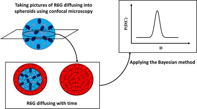
Multicellular spheroids have emerged as a robust platform to model tumor growth and are widely used for studying drug sensitivity. Diffusion is the main mechanism for transporting nutrients and chemotherapeutic drugs into spheroids, since they are typically avascular. In this study, the Bayesian inference was used to solve the inverse problem of determining the light attenuation coefficient and diffusion coefficient of Rhodamine 6G (R6G) in breast cancer spheroids, as a mock drug for the tyrosine kinase inhibitor, Neratinib. Four types of breast cancer spheroids were formed and the diffusion coefficient was estimated assuming a linear relationship between the intensity and concentration. The mathematical model used for prediction is the solution to the diffusion problem in spherical coordinates, accounting for the light attenuation. The Gaussian likelihood was used to account for the error between the measurements and model predictions. The Markov Chain Monte Carlo algorithm (MCMC) was used to sample from the posterior. The posterior predictions for the diffusion and light attenuation coefficients were provided. The results indicate that the diffusion coefficient values do not significantly vary across a HER2+ breast cancer cell line as a function of transglutaminase 2 levels, even in the presence of fibroblast cells. However, we demonstrate that different diffusion coefficient values can be ascertained from tumorigenic compared to nontumorigenic spheroids and from nonmetastatic compared to post-metastatic breast cancer cells using this approach. We also report agreement between spheroid radius, attenuation coefficient, and subsequent diffusion coefficient to give evidence of cell packing in self-assembled spheroids. The methodology presented here will allow researchers to determine diffusion in spheroids to decouple transport and drug penetration changes from biological resistivity.

Graphical Abstract

1. Introduction

Cancer is one of the leading causes of death worldwide, with breast cancer (BC) being the most commonly diagnosed and the second most common cause of cancer mortality in women [1]. A plethora of techniques have been developed to study cancer progression in vitro, including scaffold-based and non-scaffold-based models [2–4]. Among the non-scaffold-based methods, cellular spheroids are widely used, as they are a simple yet robust 3D model [5–7]. Spheroids are 3D spherical cell clusters that form by cell aggregation in suspended media [8]. Spheroids can mimic tumors in that they can capture the known layers of varying proliferation as well as the gradients of acidity, oxygen, and solutes [9, 10]. In addition to studying tumor development, spheroids are often used for in vitro drug screening. Since spheroids are typically avascular cell assemblies, diffusion is the major mechanism for nutrient and drug delivery to the cells residing at different radii [11]. Fick’s law of diffusion is generally used to model the diffusion of drugs or nutrients in spheroids [12–14]. As a result, determining the magnitude of the diffusion coefficient is crucial for modeling drug penetration.

Previous studies have modeled the diffusion of several nutrients and drugs into spheroids [15, 16]. Generally, a Fickian diffusion equation with an average constant diffusivity is utilized for capturing the diffusion in spheroids. Indeed, the cellular environment is composed of cells and extracellular matrix, implying a porous structure. By defining an effective diffusivity, the porosity can be implicitly captured in the effective diffusion coefficient leading to the mass diffusion equation with a constant diffusion coefficient [17–20]. However, these works are concerned with forward problems, such as an unknown concentration field that is obtained from a known diffusion coefficient. Standard forward diffusion problems are often well-posed, leading to a unique and stable solution.

There is a myriad of studies that have numerically studied drug delivery as a forward problem both in nano/micro-scale through molecular dynamics [21–23] and in macro-scale through the discretization of the continuum diffusion equation [24, 25]. However, determining the diffusion coefficient of drug based on the given concentration field is considered to be an inverse problem, which has not gained as much attention. Inverse problems are often ill-posed and difficult to directly solve. Accordingly, many methods have been developed to regularize this ill-posedness [26]. Among the regularization methods, the Bayesian approach not only estimates the unknown variable of interest, but it provides the uncertainty of estimation. The Bayesian approach can be implemented to determine the unknown constants in problems involving diffusion. Specifically, Bayesian inference has been widely used to determine the diffusion coefficient in different physical applications, including cosmic ray propagation [27, 28], thermal diffusion [29–31], and mass diffusivity for diffusion of beads in hydrophilic gels [32] and diffusion of biomolecules inside membrane microdomains [33]. Additionally, Markov Chain Monte Carlo (MCMC) is widely used to sample from the posterior distribution in inverse problems [34–36].

Here, we demonstrate how the mass diffusivity and light attenuation coefficients can be accurately determined for a mock drug diffusing into cancer spheroids using the Bayesian approach and MCMC sampling method. Specifically, we analyzed the diffusion coefficient of Rhodamine 6G (R6G) into HER2+ BC cell spheroids with varying levels of tissue transglutaminase 2 (TG2). TG2 is an extracellular matrix crosslinking enzyme whose upregulation has been previously shown in this progression cell series to accelerate primary tumor growth and facilitate metastasis in vivo [37]. Using confocal laser microscopy, the concentration of R6G was measured as it diffused into each spheroid based on the fluorescent intensity. R6G belongs to the rhodamine branch of the fluorophore family that can easily penetrate cell membrannes compared to other dyes like fluorescein derivatives [38]. Additionally, owing to the negative potential across mitochondria, R6G accumulates in the mitochondria [38, 39](Fig. S1). R6G is similar in size to some relevant chemotherapeutics, such as the tyrosine kinase inhibitor, Neratinib. Tyrosine kinase inhibitors are often used as adjuvant therapy for HER2+ BC patients [40–42]. Understanding the extent to which diffusivity influences drug sensitivity in drug screenings is important for decoupling mechanical resistivity through drug transport from true biological resistivity of transformed cells. To our knowledge, using the Bayesian approach to quantify diffusion in cellular spheroids has not been studied before, but may provide an excellent avenue for better understanding of the drug resistivity in cancer cells in addition to providing a robust method to extracting the parameters of interest from noisy biological data.

2. Materials and methods

2.1. Reagents

All BC cell lines were kindly provided by Dr. Michael K. Wendt (Purdue University, IN) and were previously generated from human mammary epithelial (HMLE) parental cells [37, 43]. Briefly, HMLE cells were transformed by over-expression of HER2 to generate the E2 line. E2 cells cannot metastasize in vivo. Therefore, epithelial-mesenchymal transition was induced in vitro via TGF-β1 stimulation. The stably-mesenchymal cells were engrafted into the mammary fat pad of immunocompromised mice and the bone metastases were subcultured to generate the BM line. Previous work demonstrated that TG2 was part of a novel gene signature that emerged only after the cells underwent both induction and reversion of the epithelial-mesenchymal transition. TG2 expression was therefore previously manipulated in both of the cell lines. TG2 expression was downregulated in the BMs via TG2-targeted shRNAs, creating the BMshTG2 line. A separate line of the BMs was also transduced with an empty vector as a control, and used here as the BM line. TG2 was overexpressed in the E2 line, creating the E2TG2 line, with GFP-expression added to a separate line of the original E2 cells as a control [37]. Post-metastatic cells are often more resistant to chemotherapeutic drugs than the primary tumor cells, but it is unclear how much of this may be due to a physical difference, such as tighter cell-cell packing in metastases, versus clonal selection of the population throughout the stages of metastatic cascade, with differences such as TG2 expression, and if these differences can be accurately recapitulated in spheroid models. Cells were cultured in DMEM/High Glucose media with 10% fetal bovine serum, 1% penicillin/streptomycin, and 1% insulin. Human mammary fibroblasts were cultured in fibroblast basal media with 10% fetal bovine serum, and 1% penicillin/streptomycin. In coculture experiments, each cell type was grown in its corresponding media, but seeded together into the BC media for spheroid formation.

2.2. Spheroid formation

To form the spheroid, 2000 cells were seeded into 96 well round-bottom plates (Corning Spheroid Microplate, Cat. #4520) in 300 μL phenol red-free media. In coculture experiments, 1000 of each cell type was seeded in 300 μL media, giving the same total cell number. After 48 hours, cells had aggregated into spheroids. A spheroid and all media was transferred to a 96 glass bottom well plate with black walls (Cellvis, Cat. #P96-1.5H-N) for confocal microscopy. Cell seeding was staggered such that each spheroid began diffusion imaging after 48 hours. The sizes of the spheroids at the beginning of the kinetic experiment are listed in Table. 1.

Table 1:

Values for the diffusion and attenuation coefficients. “sd” and “map” stand for the standard deviation and maximum a posteriori. D and a are in μm²/s and μm⁻¹. R and ε denote the average radius in μm and porosity, respectively.

E2	${\widehat{D}}_{\text{mean}}$	${\widehat{a}}_{\text{mean}}$	sd of $\widehat{D}$	sd of $\widehat{a}$	D mean	a mean	D map	a map	R	ε
1	0.185	−0.671	0.297	0.100	0.431	0.012	0.439	0.015	153	0.482
2	−0.0391	−0.651	0.289	0.123	0.344	0.015	0.351	0.015	166	0.595
3	0.512	−1.176	0.253	0.009	0.598	0.009	0.603	0.009	167	0.602
4	0.152	−0.971	0.248	0.099	0.417	0.011	0.422	0.011	141	0.339
E2TG2
1	0.072	−0.714	0.293	0.115	0.385	0.014	0.393	0.014	204	0.804
2	0.120	−0.807	0.287	0.111	0.404	0.013	0.410	0.013	200	0.792
3	−0.006	−0.628	0.297	0.117	0.356	0.015	0.363	0.015	191	0.762
4	0.506	−1.558	0.222	0.117	0.594	0.006	0.604	0.006	230	0.863
BM
1	0.239	−1.138	0.238	0.100	0.455	0.009	0.458	0.009	169	0.626
2	−0.092	−0.547	0.289	0.104	0.326	0.017	0.331	0.017	154	0.506
3	0.206	−1.075	0.252	0.103	0.440	0.009	0.446	0.009	177	0.675
4	−0.086	−0.146	0.316	0.134	0.329	0.024	0.332	0.024	173	0.652
BMshTG2
1	0.035	−0.931	0.264	0.114	0.371	0.011	0.376	0.011	191	0.722
2	−0.036	−0.232	0.310	0.127	0.346	0.023	0.350	0.023	179	0.662
3	−0.039	−0.655	0.295	0.116	0.345	0.015	0.353	0.015	186	0.699
4	0.082	−0.682	0.284	0.098	0.388	0.015	0.394	0.015	166	0.577

2.3. Confocal laser microscopy

Diffusion of R6G into spheroids was imaged on an LSM 880 confocal microscope. To reach the final concentration of 0.032 mM, 10 μL of l mM R6G dye (Sigma-Aldrich, Rhodamine 6G, dye content 99%, C₂₈H₃₁N₂O₃Cl, molecular weight 479.01 g/mol, SKU 252433) was added to the well and gently pipette mixed. Z-stack images were taken of the spheroid using a 10x objective (100x final magnification) at 10 minute intervals for 4–6 hours. The Zeiss LSM 880 confocal microscope uses preloaded spectral data from Pubspectra by Dr. George McNamara for each dye. Using this “smart setup” technology, the R6G dye was excited with the 514 Argon laser line and emission was collected from 521–699 nm. Fig. 1 shows the images obtained for the four BC cell types at different times.

Fig. 1:

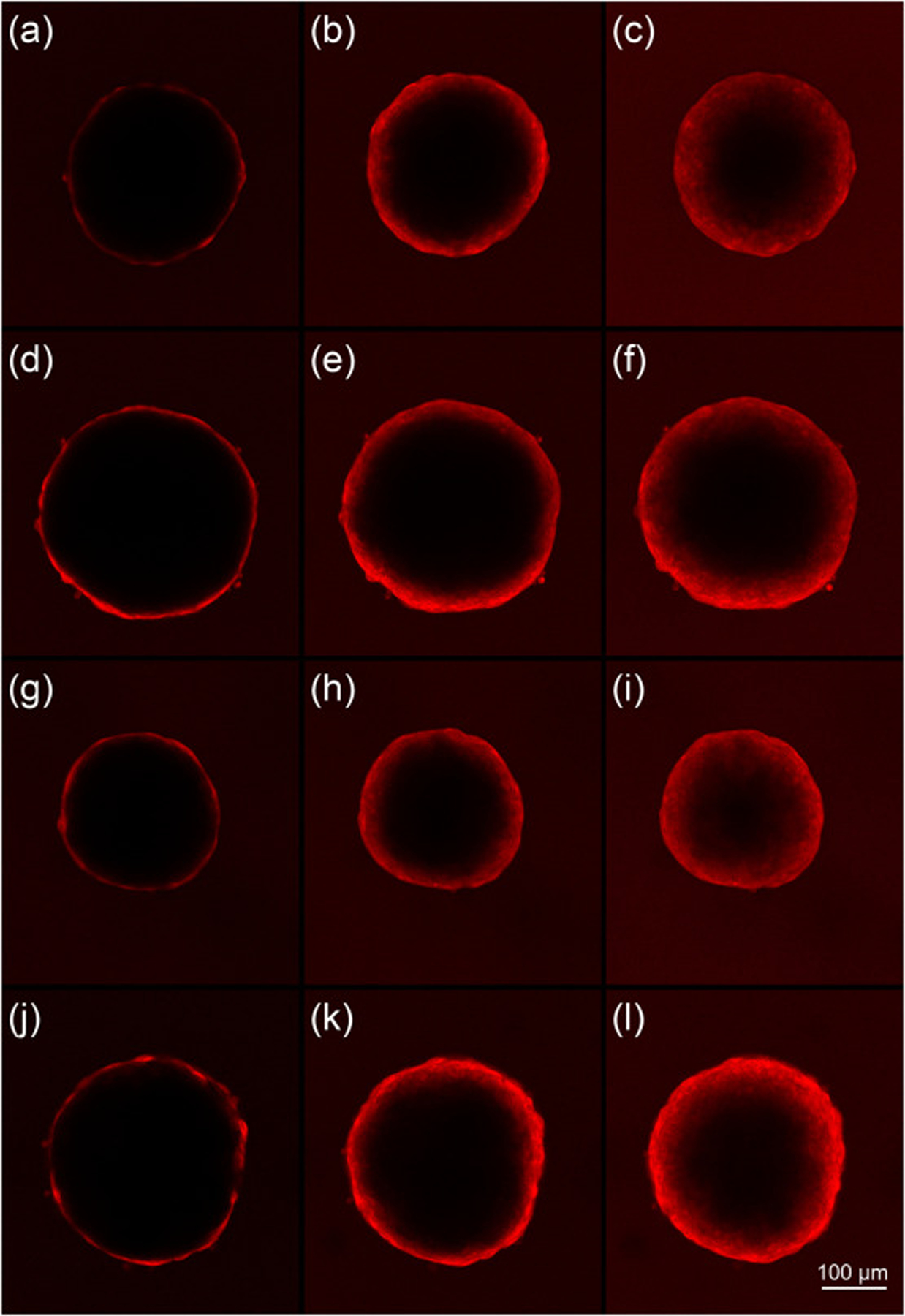
Confocal microscopy images of the E2 (a-c), E2TG2 (d-f), BM(g-i) and BMshTG2 (j-l) spheroids at 10 (left), 100 (middle), 200 (right) min after R6G was added.

2.4. Mathematical formulation

As light penetrates a medium, its intensity decreases due to absorption and scattering. As a result, the intensity, I, obtained from each image must be corrected to account for the light attenuation. R6G has a molar extinction coefficient of 8.5 × 10⁴ cm⁻¹M⁻¹ in water corresponding to the maximum absorption wavelength of λ_max = 526 nm [44]. Fluorophores have higher extinction coefficients in the membrane environment compared to water [45]. For example, R6G in 10⁻¹ M aqueous sodium dodecylsulphate (SDS) micellar solution has an extinction coefficient of 9 × 10⁴ cm⁻¹M⁻¹ corresponding to λ_max = 532.5 nm [44]. Even though the extinction coefficient of R6G in water and membrane phases is different, the difference is small ~0.5 × 10⁴ cm⁻¹M⁻¹ (~5%). As a result, in the current study, we don’t distinguish between the water and oil phases, and only consider one average coefficient with assigned uncertainty to model the light attenuation. In this experiment, images were taken at various z-positions throughout the spheroid. The position which most closely dissected the middle of the spheroid was chosen for determining the diffusion coefficient. The remaining images were utilized to determine the light attenuation through the tissue. It is expected that the fluorescent intensity for a uniform concentration field corresponding to the uniform intensity, I₀, decreases from the boundaries towards the center. There are different models in the literature to account for the light attenuation in tissues. However, based on the Beer-Lambert’s law, the exponential decay [46, 47] is the most common method used to capture light attenuation in biological samples as given in the following:

$$I=I_0\text{ exp}(-az),$$ (1)

where a and z stand for the attenuation coefficient and the attenuation depth. The attenuation coefficient can be further decomposed into fluorescence distribution coefficient and light attenuation coefficient [48, 49]. However, in this work, the product of the attenuation and distribution coefficients are treated as a single attenuation coefficient. Spheroids, even though not exactly spherical, can be approximately treated as spheres with radius, R, and gradients only in the radial direction owing to the symmetry. Transport by diffusion is the only mechanism active in avascular tumor spheroids. In general, the diffusing molecule can diffuse into the extracellular environment, bind to the cell membrane, and diffuse into cells depending on its size. If the diffusion inside the cells is neglected, the diffusion equation for the concentration in the extracellular environment, C_e, is a function of radial position, r, and time, t, as in the following:

$$\begin{gathered} \frac{\partial C_{\text{e}}}{\partial t}=\frac{1}{r^2}\frac{\partial }{\partial r}\left(r^2{D}_{\text{e}}\frac{\partial C_{\text{e}}}{\partial r}\right) \\ -k_{\text{bind}}\left(B_{\text{max}}-C_{\text{bind}}\right),C_{\text{e}}={C_0|}_{r=R},0\le r\le R, \end{gathered}$$ (2)

where D_e, k_bind, C_bind, and R stand for the diffusion coefficient, binding rate, concentration of the molecule of interest that binds to the cell membranes, and the radius of the spheroid. The maximum binding capacity, B_max, limits the number of molecules that can bind to the cell membrane. The binding process is represented as follows:

$$\frac{\partial C_{\text{bind}}}{\partial t}=k_{\text{bind}}\left(B_{\text{max}}-C_{\text{out}}\right).$$ (3)

The R6G molecule is relatively small and easily can pass through the cell membrane. As a result, the binding term, C_bind, can be neglected because k_bind = 0 [39]. Indeed, R6G molecules can enter the cell membrane and diffuse inside the cells (Fig. S1). As a result, R6G diffusion can be represented by Fick’s law of diffusion with the effective diffusivity, D_eff, given as follows:

$$\frac{\partial C}{\partial t}=\frac{1}{r^2}\frac{\partial }{\partial r}\left(r^2{D}_{\text{eff}}\frac{\partial C}{\partial r}\right),C={C_0|}_{r=R},0\le r\le R,$$ (4)

where D_eff is the effective diffusion coefficient. In general, the effective diffusivity depends on the porosity, ε, as well as the diffusivity in the extracellular environment, D_e, and inside the cells, D_i. Models like suspended permeable spheres can capture this dependence [50]. Furthermore, the porosity values likely change as a function of radial position since the cell sizes and packing can vary considerably across the radius of spheroids. Therefore, the effective diffusivity may also change with radial position. Determining the radial porosity of the spheroids requires high-resolution imaging with impermeable dyes to locate the cell boundaries, however, which is beyond the scope of this study. To get a rough estimation of the average porosity, ε, though, we used the average volume of each cell type, V_cell, the number of cells seeded, N, and the total volume of the spheroids, V_tot, to calculate the porosity in the entire spheroids as follows:

$$\epsilon =1-\frac{N{V}_{\mathit{\text{cell}}}}{V_{\mathit{\text{tot}}}},$$ (5)

where the values are listed in Table 1. The volume for each cell type was averaged from 5–9 separate passages of said cell type directly before seeding for a spheroid experiment and was calculated based on the diameters obtained by the Luna FL automatic cell counter (Logos Biosystems). Additionally, in the current study, we are not concerned with how diffusivity is related to each parameter, ε, D_e, and D_i, or how changes in each specifically alter the effective diffusivity. Instead, we focus on how the effective diffusivity itself changes for different spheroid types, which captures the net changes that happen in the diffusivity due to the cell type or presence/absence of TG2. Following the previous studies [12, 39], ε, D_e, and D_i are considered not to be a function of position leading to a constant effective diffusivity for each spheroid category as in the following:

$$D_{\text{eff}}=f\left(\epsilon ,D_{\text{e}},D_{\text{i}}\right)=\text{ cte}.$$ (6)

For the sake of convenience, we drop the term “effective” and the corresponding subscript and simply use the diffusion coefficient, D. The analytical solution to equation 4 is given as follows:

$$\frac{C}{C_0}=1+\frac{2R}{r\pi }\sum _{n=1}^{\infty }\frac{{(-1)}^n}{n}\text{sin}\left(\frac{n\pi r}{R}\right)\text{ exp }\left(-{(\frac{n\pi }{R})}^{2}Dt\right).$$ (7)

As we will show, since the fluorescent intensity is proportional to the concentration, it is valid to assume that C stands for the light intensity. Having considered an exponential light attenuation, the measured concentration, C_m, can be modeled as follows:

$$\frac{C_m}{C_0}=\text{exp}(-az)\left[1+\frac{2R}{r\pi }\sum _{n=1}^{\infty }\frac{{(-1)}^n}{n}\text{ sin }\left(\frac{n\pi r}{R}\right)\text{ exp }\left(-{(\frac{n\pi }{R})}^{2}Dt\right)\right].$$ (8)

In this study, we use the normalized average value of concentration at different time steps as our experimental data. Since the images correspond to concentration at the plane passing through the center of the spheroid, the normalized average concentration, $\widehat{C}$ , in the mid plane is calculated as follows:

$$\widehat{C}=\frac{1}{\pi R^2}{\int }_0^{R}2\pi r\frac{C_m}{C_0}dr.$$ (9)

The above integral can be solved numerically.

2.5. Bayesian formulation

The variables of interest are the diffusion coefficient and the attenuation coefficient. In defining the variables, it is fruitful to modify them such that they reflect certain constraints like remaining positive or negative. In the current work, to make sure that the coefficients remain positive, we use a logarithmic function to define a new vector of variables x = [x₁, x₂] as follows:

$$x_1=\text{log}\left(\frac{D}{D_0}\right)=\widehat{D},x_2=\text{log}\left(\frac{a}{a_0}\right)=\widehat{a},$$ (10)

where D₀ and a₀ are any arbitrary initial positive guess. This logarithmic function ensures that D and a have the same sign as D₀ and a₀, thereby they remain positive.

Bayes’ theorem states that the observed data vector, y, can be related to the parameter of interest, x, through:

$$p(\mathbf{\text{x}}\mid \mathbf{\text{y}})=\frac{p(\mathbf{\text{y}}\mid \mathbf{\text{x}})p(\mathbf{\text{x}})}{\int p(\mathbf{\text{y}}\mid \mathbf{\text{x}})p(\mathbf{\text{x}})d\mathbf{\text{x}}},\int p(\mathbf{\text{y}}\mid \mathbf{\text{x}})p(\mathbf{\text{x}})d\mathbf{\text{x}}=Z.$$ (11)

In the above equation, p(x|y) denotes the posterior knowledge about the parameter of interest, x. The term p(y|x) denotes the likelihood and p(x) is the prior probabilistic knowledge about x. The integral term, Z, is the normalizing constant, which is referred to as partition function. The likelihood accounts for the deviations of the model from the actual results. Indeed, it is the measure of the difference between the observed data and the model prediction. Several sources may lead to errors in our predictive modeling. The major source for the error is the pixel noise that can be attributed to environmental factors and photon noises. Another factor contributing to the deviation of predictions from the experiment is the assumption that the fluorescent intensity directly represents the concentration. This is an approximation, but is valid for low concentrations, such as those within this study, as we will demonstrate in section 3.1. The summation of all errors can be nested in a single noise term, ϵ, which relates the model prediction f(x) to the observed data as in the following:

$$y=f(\mathbf{\text{x}})+ϵ.$$ (12)

A proper way to model the noise is to assign a normal or Gaussian distribution, which can effectively model the random noises.

$$ϵ=\mathcal{N}\left(0\mid {\sigma }^2\right).$$ (13)

In the above equation, σ denotes the standard deviation. This Gaussian noise can be manifested in the likelihood of the data vector with N independent observations p(y|x) through a normal distribution as the following:

$$p(\mathbf{\text{y}}\mid \mathbf{\text{x}})=\prod _{i=1}^{N}p\left(y_i\mid \mathbf{\text{x}}\right)=\prod _{i=1}^N\mathcal{N}\left(f_i(\mathbf{\text{x}})\mid {\sigma }_i\right).$$ (14)

Assuming a constant deviation, σ, for all the independent observations, the likelihood can be simplified as follows.

$$p(\mathbf{\text{y}}\mid \mathbf{\text{x}})\propto \text{exp}\left(\frac{\sum _{i=1}^N\left(y_i-f_i{(\mathbf{\text{x}})}^2\right)}{2{\sigma }^2}\right).$$ (15)

Based on how accurate the model prediction is, the values of noise variance can vary widely. In this work, since the model prediction f(x) and experimental data is in the range [0, 1] and the data are noisy, we assumed the variance of the difference between the model prediction and the experimental data to be 0.1 corresponding to σ² = 0.01. Finding the posterior p(x|y) is the most challenging part in Bayesian inference since the Z term is not generally analytically available, except for some few cases. A common method to circumvent the difficulties associated with the direct calculation of the partition function is to use MCMC to sample from the posterior. In the current work, we use the No-U-Turn Sampler (NUTS) of PyMC3 to sample from the posterior. The open-source probabilistic programming package, PyMC3, was utilized to perform the Bayesian analysis, which is available for free use in Python [51]. The NUTS sampler is an MCMC-based method that utilizes the Hamiltonian Monte Carlo method. NUTS automatically adjusts the number of steps per sample. Further details about this method can be found in the work by Hoffman et al [52].

2.6. Prior Knowledge

If there is not any prior information available regarding the parameter of interest, uninformative priors, such as simply beginning with a uniform distribution can be used as a starting point. However, informative priors can be used when there is sufficient prior knowledge about the parameter of interest. Having an informative prior typically increases the efficiency of the model by reducing the number of iterations required to converge on the correct distribution. [53]. In the current work, a normal prior, which is considered to be an informative prior is used. The normal prior is given as follows.

$$p\left(x_i\right)=\mathcal{N}\left(0\mid {\gamma }_i^2\right)=\frac{1}{\sqrt{2\pi {\gamma }_i^2}}\text{exp }\left(-\frac{x_i}{2{\gamma }_i^2}\right),$$ (16)

where γ_i denotes the standard deviation corresponding to the variable of interest. The standard deviation can be assumed to have a constant value or follow a distribution. In the current study, constant values were assumed for γ₁ and γ₂. Having separated the cellular spheroids into two parts including the cells and matrix, Astrauskas et al. [39], calculated the values of the diffusion coefficient of the R6G in embryonic fibroblast spheroids to be D_cell = 0.3 μm²/s and D_matrix = 0.42 μm²/s. Based on these values, the average diffusion coefficient can be expressed as D_ave = 0.357 μm²/s. We used this value for D₀ and approximately 30% of D₀ for the standard deviation leading to ${\gamma }_1^2\approx 0.1$ . Additionally, as we will show in the next section, we assumed a₀ = 0.028 with the variance of ${\gamma }_2^2\approx 0.1$ . The prior probability density plot for the attenuation and diffusion coefficient is shown in Fig. 2.

Fig. 2:

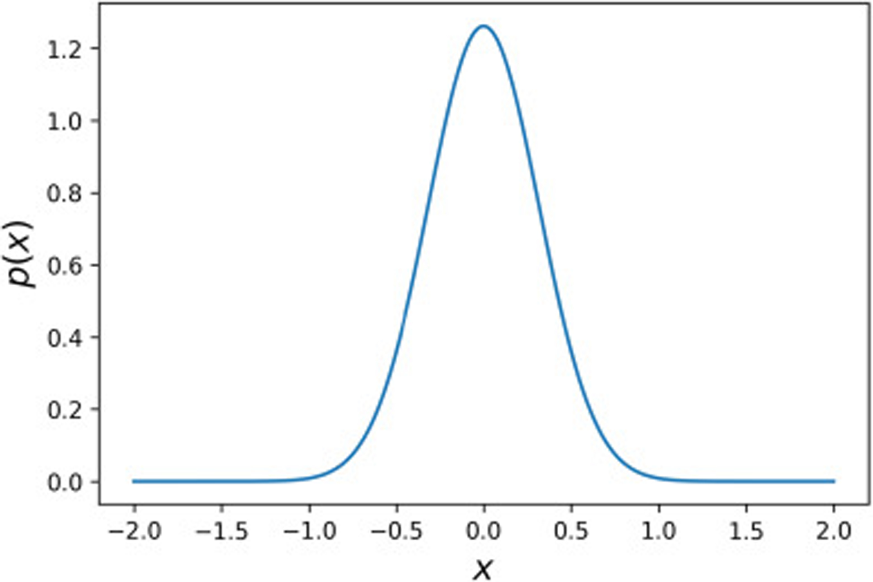
Prior probability density distribution for both $x=\widehat{a}$ and $x=\widehat{D}$ with the mean of 0 and the variance of γ² = 0.1.

2.7. Statistical Analysis

Statistical significance was determined using a single factor analysis of variance or two-sided T tests, where the data met the assumptions of the tests. The data was analysed for outliers using the Grubbs test, where no outliers were found, and the variance was analysed before a given T test using the Leven Test for Equality of Variances. p values of < 0.05 were considered significant.

3. Results and Discussion

3.1. Calibration curve

Our modeling is based on the assumption that the concentration is proportional to the fluorescent intensity. To verify this assumption, we present the calibration curve for R6G as shown in Fig. 3. Using the same 1mM stock of R6G as for the spheroid studies, a serial dilution from 0.05 – 0.00156 mM, with halved concentration at each step, was used. Samples were imaged every 30 minutes for two hours at one height in the same type of black-walled glass bottom well plate used for the spheroid imaging sets. At the end of the kinetic run, Z stacks with a 24 μm interval were taken as well. The curve shows the light intensity as a function of concentration for R6G in phosphate-buffered saline (PBS), and the solution of olive oil-Tween 20 (50–50% volume) to imitate the cellular environment. For a relatively large concentration range (0.00156–0.05 mM), as shown in the two top panels in Fig. 3, the light intensity non-linearly changes with the concentration with the polynomial fit of second degree predicting the points with a high accuracy suggesting that a linear fit cannot be a good predictor for this range. However, as shown in the two bottom panels of Fig. 3, for the smaller concentration range (0.00156–0.03 mM), the light intensity can be assumed to be proportional to the concentration as R² = 0.99. In this study, the maximum R6G concentration is 0.032 mM at the boundary, suggesting that a linear relationship between concentration and the fluorescent intensity can be safely assumed throughout the spheroids.

Fig. 3:

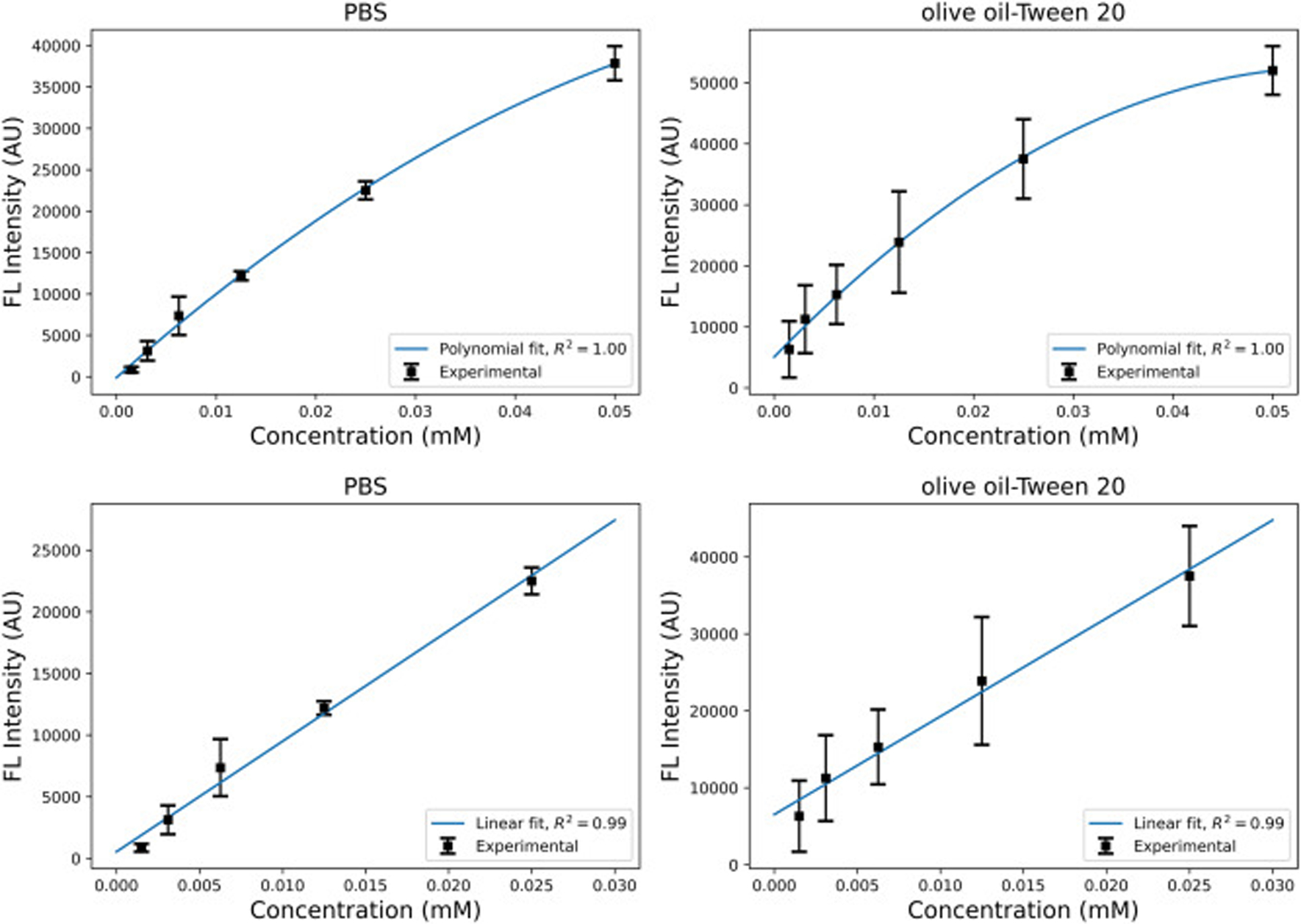
The calibration curve for the R6G in PBS and olive oil-Tween 20 (50–50% volume) solutions. The two top graphs demonstrate the polynomial second degree fit for the concentration range of 0.00156–0.05 mM. The two bottom graphs demonstrate the linear fit for the concentration range of 0.00156–0.03 mM.

3.2. Attenuation coefficient

In order to get the prior information for the value of the attenuation coefficient, it would be very helpful to capture longer kinetic experiments to ensure that R6G reaches steady state at the center. However, because the cells were not incubated during imaging, prolonged studies could be affected by significant cell death, which would change the spheroid integrity and thus alter the calculated light attenuation. We chose to increase the imaging time from 4 to 6 hours, at which point significant penetration of dye could be seen in the center of the spheroid. We then compared the concentration at the spheroid boundaries and centers for each scenario. The images were taken at different planes that were 20 μm apart. To find the average intensity at different stacks, an area of 20 × 20 pixels around the center of spheroids was considered at each stack and the average intensity was calculated. Fig. 4 shows the logarithm of the average intensity as a function of depth for the four types of spheroids that were used in this study. The slope of these lines denotes the attenuation coefficient. The mean value obtained for the attenuation coefficient is 0.028 μm⁻¹. The noticeable variation in the mean value of a can be attributed to the relatively large noise in the intensity values and pixel saturation. Additionally, an exponential decay for the intensity is an approximation showing different levels of accuracy for different spheroids. However, all in all, the coefficient of determination has acceptable values (R² > 0.9) as shown in Fig. 4. This mean value is used in our modeling as the mean value of prior. However, since these mean values show large variations, we assigned a large standard deviation to the prior, i.e. ${\gamma }_2^2=0.1$. Furthermore, to confirm that validity of the light attenuation coefficient range calculated, we compared the coefficient obtained by the R6G-soaked spheroids with a spheroid of dTomato-transduced cells. The MCF10CA1a triple negative BC cell line previously underwent lentiviral transduction to stably express dTomato [54]. Because each cell expresses fluorescence, there is no dye concentration gradient, and any fluorescence gradient would be fully attributed to light attenuation through the spheroid. . The images of the spheroids and the intensity vs depth curves are provided in Fig. S3 and S4. The values of the radius and attenuation coefficients are also provided in Table S1. The results showed the average values of the attenuation coefficient 0.029 μm⁻¹. which is in agreement with the prior value obtained for the R6G-dyed spheroids.

Fig. 4:

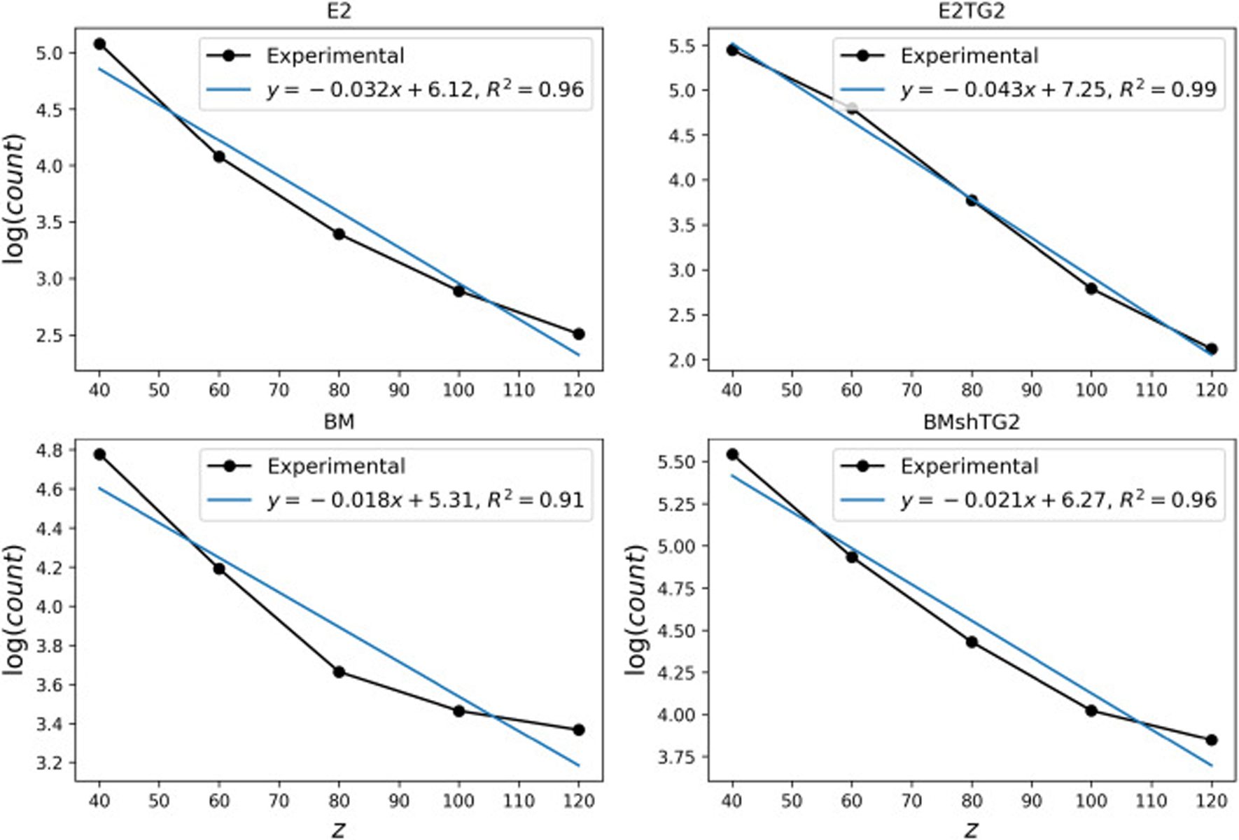
Logarithm of light intensity as a function of depth, z(μm), for a spheroid of each cell type. The distance z is measured from a plane tangent to the spheroids.

3.3. Sampling from the posterior distributions

For all four cell types, the experiments were repeated four times and sampling was applied to each spheroid. The package PyMC3 was used to generate samples from the posterior using the NUTS sampler. When sampling from the posterior, it is crucial to have autocorrelation as minimum as possible. Otherwise, the independence of the sampled points is not satisfied. The autocorrelation, R, for a dataset y with N elements and the mean of $\overline{y}$ is given as follows.

$$R=\frac{1}{N-l}\sum _{n=1}^{N-l}\left(y_n-\overline{y}\right)\left(y_{n+l}-\overline{y}\right)l=1:N.$$ (17)

After initial sampling, the first initial 3000 samples were burned and the samples were thinned accordingly, leaving 5000 samples with minimized autocorrelation. This sampling procedure was repeated for all the spheroids. Here, we present the autocorrelation plots for one type of spheroid, which are representative for the other spheroids as well. Fig. 5 shows the autocorrelation plots for the 100 number of draws. It is evident that the burned and thinned dataset has the desirable autocorrelation.

Fig. 5:

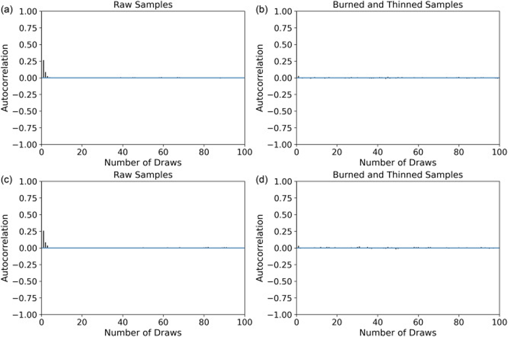
Autocorrelation plots for the $\widehat{D}$ ((a) raw samples (b) burned and thinned samples) and $\widehat{a}$ ((c) raw samples (d) burned and thinned samples). Data corresponds to sampling from the posterior of a spheroid in the E2 category using the NUTS sampler.

3.4. Estimation of the coefficients

The same prior distribution was assumed for all spheroids. The posterior plots for the diffusion coefficients of the spheroids are shown in Fig. 6. Despite the noisy nature of these data, the mean and the maximum posterior results are in a close range as shown in Table 1. Standard deviations are also listed to give insight into the confidence interval. According to these plots, although some distributions are relatively different for different spheroids, they can still be represented in a close range. Indeed, the mean values obtained for the diffusion coefficient are in the range 0.3 − 0.6 μm²/s. This range is similar to what Anissimov et al. [55] reported for the diffusion of rhodamine B in stratum corneum. Our results suggest no statistically significant difference in diffusion as a function of TG2 levels.

Fig. 6:

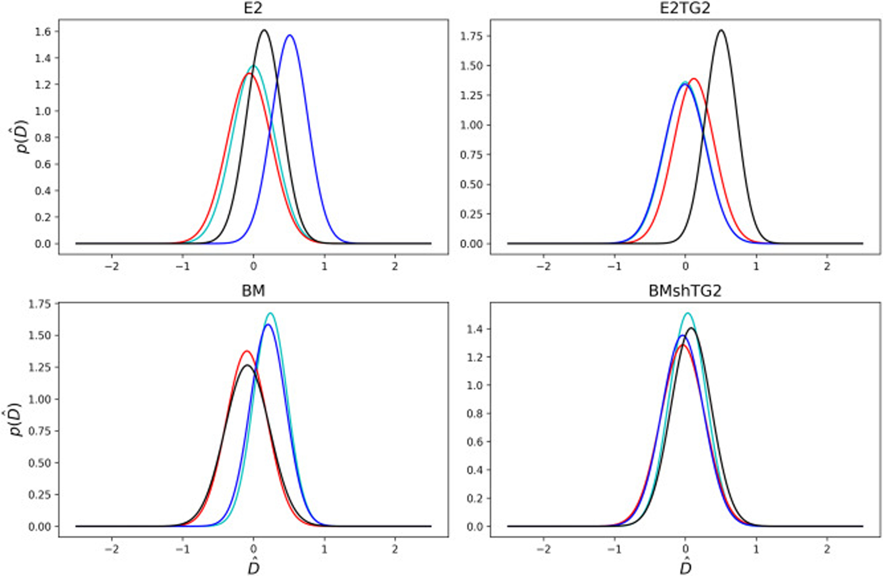
Probability density plots of the posterior predictions for the non-dimensional diffusion coefficient, $\widehat{D}$ , for all the spheroids. Each line corresponds to a unique spheroid tested for each cell, with four spheroids tested in each category. Different colors help distinguish overlapping graphs.

Fig. 7 shows the posterior distributions for the attenuation coefficient. The mean and standard deviations are also listed in Table 1. The distributions have almost the same standard deviations; however, with different means. The mean values obtained for the attenuation coefficients are in the range 0.005 − 0.025 μm⁻¹. The size of spheroids vary between 150 and 200 μm. Given that the different cell types may have varied proliferation rates during the 48 hour aggregation period, and that the cell surface density is a function of radius owing to the spherical geometry, values for the mean attenuation coefficients vary noticeably. By implementing the Bayesian approach, we were able to calculate the diffusion and attenuation coefficients despite this relatively noisy data typical of biological experiments.

Fig. 7:

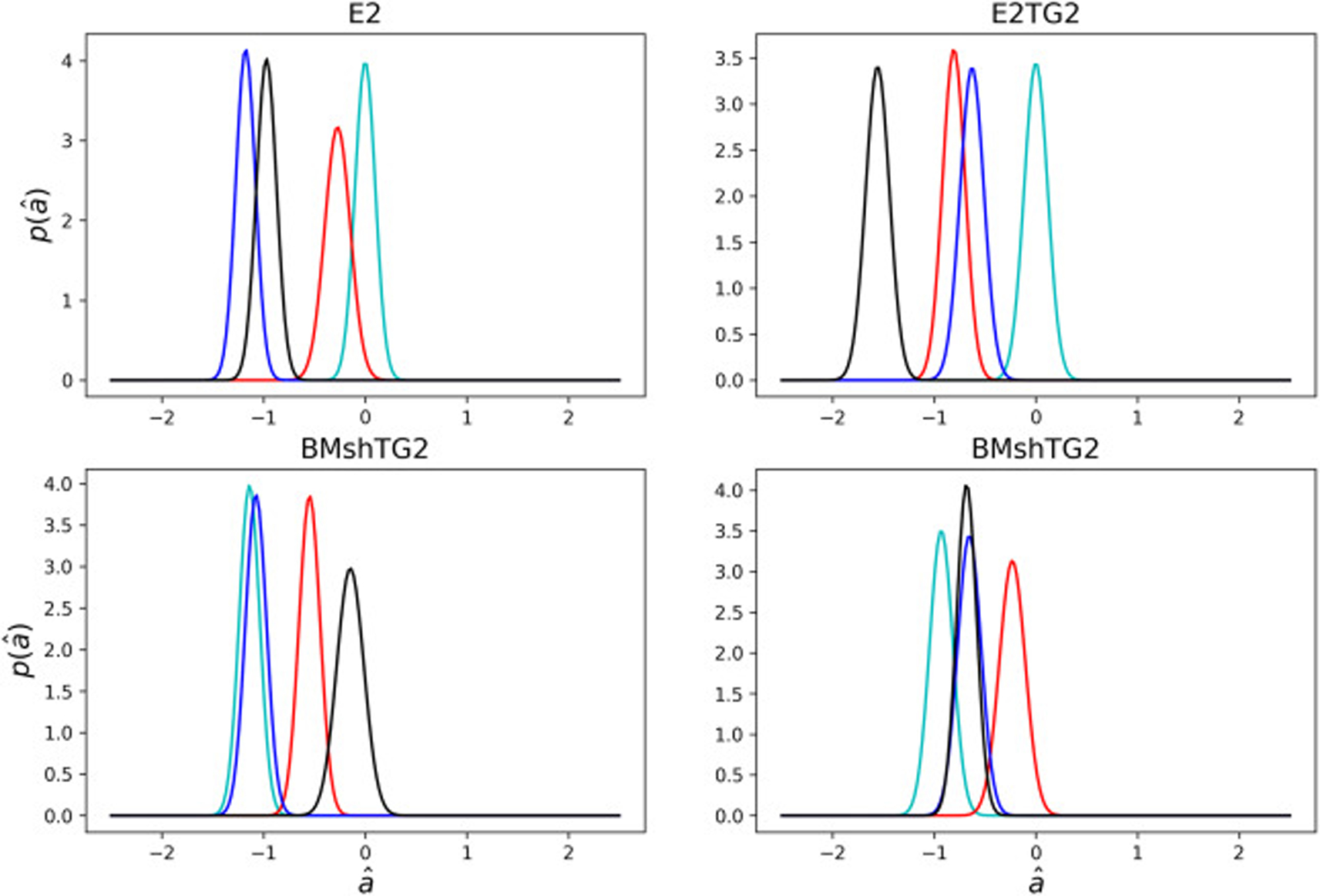
Probability density plots of the posterior predictions for the non-dimensional attenuation coefficient, $\widehat{a}$ , for all the spheroids Each line corresponds to a unique spheroid tested for each cell, with four spheroids tested in each category. Different colors help distinguish overlapping graphs.

3.5. Posterior predictive distribution of the experimental data

The Bayesian analysis not only provides information about the values of the unknown coefficients, but it also provides the posterior prediction for the values of the concentration. This is a useful tool for investigating the accuracy of the model. If $\tilde{y}$ denotes a new data point corresponding to the observed data y, according to the Bayes rule, the posterior prediction becomes as the following:

$$p(\tilde{y}\mid \mathbf{\text{y}})=\int p(\tilde{y},\mathbf{\text{x}}\mid \mathbf{\text{y}})d\mathbf{\text{x}}=\int p(\tilde{y}\mid \mathbf{\text{x}},\mathbf{\text{y}})p(\mathbf{\text{x}}\mid \mathbf{\text{y}})d\mathbf{\text{x}}$$ (18)

The posterior predictions for the values of the concentration were also calculated using PyMC3 and the mean values are shown in Fig. 8. It is evident that for some spheroids there is a great match between model prediction and experimental data, while in others the model cannot strongly capture the data due to the noisy nature of the pixel intensities. However, for all of these models, we assigned a rather large standard deviation in the prior such that all the data and prediction lie in the 95% confidence interval.

Fig. 8:

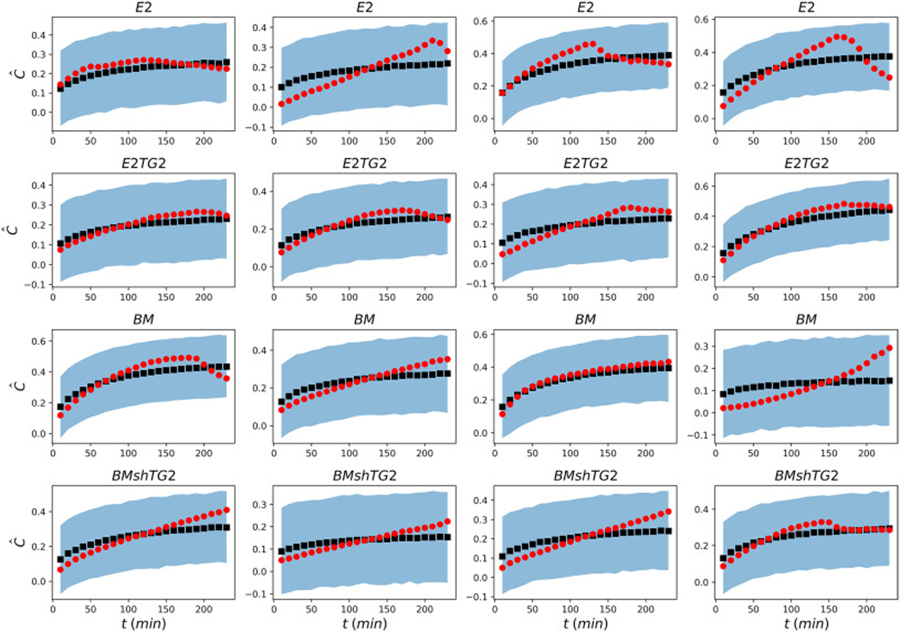
Comparison of the experimental data (red circles) with the mean posterior prediction (black squares) of the concentration. The light blue region displays 95% confidence interval of the posterior prediction for the values of concentration.

As mentioned in the previous section, the intensity values are normalized with respect to the maximum intensity. It is expected that in the absence of attenuation, the average normalized concentration reaches one after sufficient time passes. However, it is clear from Fig. 8 that the light attenuation reduces the overall average concentration leading to $\widehat{C}$ values smaller than one. Taking into account the light attenuation, Bayesian analysis is capable of predicting the experimental data from relatively noisy input data with great accuracy.

3.6. Posterior predictive distribution after fibroblast incorporation

TG2 has been shown to crosslink extracellular matrices, including crosslinking fibronectin on the surface of extracellular vesicles from this BC progression series [37]. However, our recent work suggests that BC cells cannot organize secreted fibronectin into a fibrillar extracellular matrix without fibroblast intervention [56]. It was not previously known if changes to the extracellular matrix would significantly affect the diffusion rate of small molecule chemotherapeutics or dyes such as R6G, which readily penetrate into the cell membrane. We therefore determined the diffusion coefficient of cocultured spheroids, created with a 1:1 ratio of BC cells and human mammary fibroblasts (HMFs). Additionally, to show that the similarities observed in the diffusivity of the BC spheroids was due to true biological similarity and not an error of the methodology, we conducted experiments using fully nontumorigenic spheroids, made of 2000 HMFs as a control set (Fig. S4). As shown in Fig. S5, similar to BC cells, for the coculture spheroids and nontumorigenic spheroids, all the obtained posterior predictions lie within the 95% confidence interval, with some predictions having a better match with the experimental results.

We use the same Bayesian procedure with the Gaussian priors and likelihood as we did for the cases without HMFs to obtain the diffusion and attenuation coefficients. Similar to homogeneous spheroids made from the BM and BMshTG2 cell lines, the values of diffusivity for spheroids co-cultured with HMFs demonstrate no significant difference in the diffusion or light attenuation coefficients as a function of TG2 expression (Fig. 9, Table S1). Fig. 9 shows the average diffusion coefficient, attenuation coefficient, and spheroid radius for the 7 cellular conditions tested. We demonstrate that spheroids made with noncancerous mammary fibroblasts have a lower diffusion coefficient than the BC spheroids, with this difference being significant against the E2 and E2TG2 cell lines. These results also show that BC:HMF coculture spheroids have average diffusion coefficients in between the average value for the BC cell type and the HMFs in their respective monoculture spheroid, although these values were not significantly different. Similarly, the HMF spheroids were statistically smaller than the BC spheroids, but not statistically different from the coculture spheroids due to slightly smaller sizes and/or larger variation within the two coculture groups.

Fig. 9:

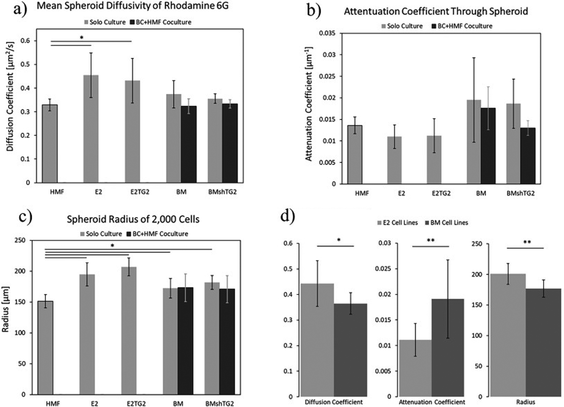
Comparison of the average a) diffusivity, D_mean b) attenuation coefficient, a_mean c) spheroid radius, R, for all of the measured spheroid types d) values of the diffusion, attenuation coefficients and the radius for the E2 and BM cell lines. * indicates p<0.05 and ** indicates p<0.01.

Lastly, we see agreement among our calculated parameters, which together give indication of how these cells pack into spheroids. For example, HMF spheroids are statistically smaller than the E2 and E2TG2 spheroids and trend with a higher attenuation coefficient, meaning that the light could not penetrate into the cellular mass as efficiently. This indicates that mammary fibroblasts can aggregate into a more compact spheroid with tighter cell:cell junctions. Those characteristics should lower the diffusion coefficient, which falls in line precisely with what our methods calculated. We see this same agreement among the average values of the pre-metastatic E2 cell lines compared with the post-metastatic BM cell lines. Fig. 9D shows combined values for the two E2 and BM lines tested as TG2 levels did not have a significant difference for any parameter due to the diffusion nature of a small molecule like R6G that passes easily through the cell membrane. Here we can see that after undergoing epithelial-mesenchymal transition and the reverse mesenchymal-epithelial transition, the post-metastatic BM cells will pack more tightly, creating spheroids that are statistically smaller, with larger attenuation coefficients, and smaller diffusion coefficients than their pre-metastatic parental counterparts, despite the two cell lines being phenotypically indistinguishable using traditional 2D culturing methods.

4. Conclusion

In this study, the concentration of the fluorescent dye, R6G, was measured at different time steps, using the fluorescence intensity captured by confocal microscopy, as the dye diffused into spheroids of several cell types.. Then, the Bayesian inference was utilized to solve the inverse problem of determining the diffusion and attenuation coefficients from the known concentration values. We presented the calibration curve of R6G, which demonstrates that the fluorescent intensity is proportional to the concentration values at the concentration range of interest. The model likelihood and the prior distribution for the coefficients were assumed to follow a normal distribution. MCMC was used to sample from the posterior and the mean values with the associated uncertainties were obtained. We obtained diffusion coefficients in the range of 0.3 − 0.6 μm²/s for each spheroid. These values are consistent with previously reported values for spheroids, implying the effectiveness of Bayesian analysis in solving inverse problems with noisy data. These values also showed that the diffusion coefficient of R6G was irrespective of TG2 level, but did differ between BC and noncancerous spheroids as well as between the nonmetastatic parental cells and the corresponding bone metastasis cells from the same BC progression series. This methodology can be applied to a range of cell types and fluorescent markers to compute diffusion rates of spheroids and other cell mass as long as the concentration of dye of interest in the media is known. Additionally, this methodology can also be applied to spheroids formed with exogenous matrices and to spheroids containing multiple cell types. In total, this technique can therefore aid researchers in decoupling differences in diffusivity of various spheroids or engineered constructs, which would affect the bioavailability of the compound of interest, from differences in the cells’ biological/chemical response or sensitivity to the compounds of interest.

References

- [1].Siegel RL, Miller KD, Goding Sauer A, Fedewa SA, Butterly LF, Anderson JC, Cercek A, Smith RA, and Jemal A, “Colorectal cancer statistics, 2020,” CA: a cancer journal for clinicians, 2020. [DOI] [PubMed] [Google Scholar]
- [2].Moon H.-r. and Han B, “Engineered tumor models for cancer biology and treatment,” in Biomaterials for Cancer Therapeutics, pp. 423–443, Elsevier, 2020. [Google Scholar]
- [3].Xie B, Teusch N, and Mrsny R, “Comparison of two-and three-dimensional cancer models for assessing potential cancer therapeutics,” in Biomaterials for Cancer Therapeutics, pp. 399–422, Elsevier, 2020. [Google Scholar]
- [4].Costa EC, Moreira AF, de Melo-Diogo D, Gaspar VM, Carvalho MP, and Correia IJ, “3d tumor spheroids: an overview on the tools and techniques used for their analysis,” Biotechnology advances, vol. 34, no. 8, pp. 1427–1441, 2016. [DOI] [PubMed] [Google Scholar]
- [5].Sun Q, Tan SH, Chen Q, Ran R, Hui Y, Chen D, and Zhao C-X, “Microfluidic formation of coculture tumor spheroids with stromal cells as a novel 3d tumor model for drug testing,” ACS Biomaterials Science & Engineering, vol. 4, no. 12, pp. 4425–4433, 2018. [DOI] [PubMed] [Google Scholar]
- [6].Tong WH, Fang Y, Yan J, Hong X, Singh NH, Wang SR, Nugraha B, Xia L, Fong ELS, Iliescu C, et al. , “Constrained spheroids for prolonged hepatocyte culture,” Biomaterials, vol. 80, pp. 106–120, 2016. [DOI] [PubMed] [Google Scholar]
- [7].Charoen KM, Fallica B, Colson YL, Zaman MH, and Grinstaff MW, “Embedded multicellular spheroids as a biomimetic 3d cancer model for evaluating drug and drug-device combinations,” Biomaterials, vol. 35, no. 7, pp. 2264–2271, 2014. [DOI] [PMC free article] [PubMed] [Google Scholar]
- [8].Engelberg JA, Ropella GE, and Hunt CA, “Essential operating principles for tumor spheroid growth,” BMC systems biology, vol. 2, no. 1, p. 110, 2008. [DOI] [PMC free article] [PubMed] [Google Scholar]
- [9].Moshksayan K, Kashaninejad N, Warkiani ME, Lock JG, Moghadas H, Firoozabadi B, Saidi MS, and Nguyen N-T, “Spheroids-on-a-chip: Recent advances and design considerations in microfluidic platforms for spheroid formation and culture,” Sensors and Actuators B: Chemical, vol. 263, pp. 151–176, 2018. [Google Scholar]
- [10].Nath S and Devi GR, “Three-dimensional culture systems in cancer research: Focus on tumor spheroid model,” Pharmacology & therapeutics, vol. 163, pp. 94–108, 2016. [DOI] [PMC free article] [PubMed] [Google Scholar]
- [11].Mehta G, Hsiao AY, Ingram M, Luker GD, and Takayama S, “Opportunities and challenges for use of tumor spheroids as models to test drug delivery and efficacy,” Journal of controlled release, vol. 164, no. 2, pp. 192–204, 2012. [DOI] [PMC free article] [PubMed] [Google Scholar]
- [12].Gao Y, Li M, Chen B, Shen Z, Guo P, Wientjes MG, and Au JL-S, “Predictive models of diffusive nanoparticle transport in 3-dimensional tumor cell spheroids,” The AAPS journal, vol. 15, no. 3, pp. 816–831, 2013. [DOI] [PMC free article] [PubMed] [Google Scholar]
- [13].Achilli T-M, McCalla S, Meyer J, Tripathi A, and Morgan JR, “Multilayer spheroids to quantify drug uptake and diffusion in 3d,” Molecular pharmaceutics, vol. 11, no. 7, pp. 2071–2081, 2014. [DOI] [PMC free article] [PubMed] [Google Scholar]
- [14].Ward JP and King JR, “Mathematical modelling of drug transport in tumour multicell spheroids and monolayer cultures,” Mathematical biosciences, vol. 181, no. 2, pp. 177–207, 2003. [DOI] [PubMed] [Google Scholar]
- [15].McMurtrey RJ, “Analytic models of oxygen and nutrient diffusion, metabolism dynamics, and architecture optimization in three-dimensional tissue constructs with applications and insights in cerebral organoids,” Tissue Engineering Part C: Methods, vol. 22, no. 3, pp. 221–249, 2016. [DOI] [PMC free article] [PubMed] [Google Scholar]
- [16].Carr EJ and Pontrelli G, “Modelling mass diffusion for a multi-layer sphere immersed in a semi-infinite medium: application to drug delivery,” Mathematical biosciences, vol. 303, pp. 1–9, 2018. [DOI] [PubMed] [Google Scholar]
- [17].Khanafer K and Vafai K, “The role of porous media in biomedical engineering as related to magnetic resonance imaging and drug delivery,” Heat and mass transfer, vol. 42, no. 10, p. 939, 2006. [Google Scholar]
- [18].Aleksandrova A, Pulkova N, Gerasimenko T, Anisimov NY, Tonevitskaya S, and Sakharov D, “Mathematical and experimental model of oxygen diffusion for heparg cell spheroids,” Bulletin of experimental biology and medicine, vol. 160, no. 6, pp. 857–860, 2016. [DOI] [PubMed] [Google Scholar]
- [19].Chariou PL, Lee KL, Pokorski JK, Saidel GM, and Steinmetz NF, “Diffusion and uptake of tobacco mosaic virus as therapeutic carrier in tumor tissue: effect of nanoparticle aspect ratio,” The Journal of Physical Chemistry B, vol. 120, no. 26, pp. 6120–6129, 2016. [DOI] [PMC free article] [PubMed] [Google Scholar]
- [20].Jiang Y, Pjesivac-Grbovic J, Cantrell C, and Freyer JP, “A multiscale model for avascular tumor growth,” Biophysical journal, vol. 89, no. 6, pp. 3884–3894, 2005. [DOI] [PMC free article] [PubMed] [Google Scholar]
- [21].Asadzadeh H, Moosavi A, and Arghavani J, “The effect of chitosan and peg polymers on stabilization of gf-17 structure: A molecular dynamics study,” Carbohydrate polymers, vol. 237, p. 116124, 2020. [DOI] [PubMed] [Google Scholar]
- [22].Forrey C, Saylor DM, Silverstein JS, Douglas JF, Davis EM, and Elabd YA, “Prediction and validation of diffusion coefficients in a model drug delivery system using microsecond atomistic molecular dynamics simulation and vapour sorption analysis,” Soft Matter, vol. 10, no. 38, pp. 7480–7494, 2014. [DOI] [PubMed] [Google Scholar]
- [23].Luo Z and Jiang J, “ph-sensitive drug loading/releasing in amphiphilic copolymer pae–peg: Integrating molecular dynamics and dissipative particle dynamics simulations,” Journal of controlled release, vol. 162, no. 1, pp. 185–193, 2012. [DOI] [PubMed] [Google Scholar]
- [24].Zhang A, Mi X, Yang G, and Xu LX, “Numerical study of thermally targeted liposomal drug delivery in tumor,” Journal of heat transfer, vol. 131, no. 4, 2009. [Google Scholar]
- [25].Leedale JA, Ky n JA, Harding AL, Colley HE, Murdoch C, Sharma P, Williams DP, Webb SD, and Bearon RN, “Multiscale modelling of drug transport and metabolism in liver spheroids,” Interface focus, vol. 10, no. 2, p. 20190041, 2020. [DOI] [PMC free article] [PubMed] [Google Scholar]
- [26].Stuart AM, “Inverse problems: a bayesian perspective,” Acta numerica, vol. 19, pp. 451–559, 2010. [Google Scholar]
- [27].Trotta R, Jóhannesson G, Moskalenko I, Porter T, De Austri RR, and Strong A, “Constraints on cosmic-ray propagation models from a global bayesian analysis,” The Astrophysical Journal, vol. 729, no. 2, p. 106, 2011. [Google Scholar]
- [28].Jóhannesson G, de Austri RR, Vincent A, Moskalenko I, Orlando E, Porter T, Strong A, Trotta R, Feroz F, Graff P, et al. , “Bayesian analysis of cosmic ray propagation: evidence against homogeneous diffusion,” The Astrophysical Journal, vol. 824, no. 1, p. 16, 2016. [DOI] [PMC free article] [PubMed] [Google Scholar]
- [29].Gnanasekaran N and Balaji C, “Markov chain monte carlo (mcmc) approach for the determination of thermal diffusivity using transient fin heat transfer experiments,” International journal of thermal sciences, vol. 63, pp. 46–54, 2013. [Google Scholar]
- [30].Fudym O, Orlande HRB, Bamford M, and Batsale JC, “Bayesian approach for thermal diffusivity mapping from infrared images with spatially random heat pulse heating,” in Journal of Physics: Conference Series, vol. 135, p. 012042, IOP Publishing, 2008. [Google Scholar]
- [31].Reddy BK and Balaji C, “Bayesian estimation of heat flux and thermal diffusivity using liquid crystal thermography,” International Journal of Thermal Sciences, vol. 87, pp. 31–48, 2015. [Google Scholar]
- [32].Anderson WA, Reilly PM, Moo-Young M, and Legge RL, “Application of a bayesian regression method to the estimation of diffusivity in hydrophilic gels,” The Canadian Journal of Chemical Engineering, vol. 70, no. 3, pp. 499–504, 1992. [Google Scholar]
- [33].Voisinne G, Alexandrou A, and Masson J-B, “Quantifying biomolecule diffusivity using an optimal bayesian method,” Biophysical Journal, vol. 98, no. 4, pp. 596–605, 2010. [DOI] [PMC free article] [PubMed] [Google Scholar]
- [34].Dashti M and Stuart AM, “The bayesian approach to inverse problems,” arXiv preprint arXiv:1302.6989, 2013. [Google Scholar]
- [35].Yustres Á, Asensio L, Alonso J, and Navarro V, “A review of markov chain monte carlo and information theory tools for inverse problems in subsurface flow,” Computational Geosciences, vol. 16, no. 1, pp. 1–20, 2012. [Google Scholar]
- [36].Wang J and Zabaras N, “A bayesian inference approach to the inverse heat conduction problem,” International journal of heat and mass transfer, vol. 47, no. 17–18, pp. 3927–3941, 2004. [Google Scholar]
- [37].Shinde A, Paez JS, Libring S, Hopkins K, Solorio L, and Wendt MK, “Transglutaminase-2 facilitates extracellular vesicle-mediated establishment of the metastatic niche,” Oncogenesis, vol. 9, no. 2, pp. 1–12, 2020. [DOI] [PMC free article] [PubMed] [Google Scholar]
- [38].Mottram LF, Forbes S, Ackley BD, and Peterson BR, “Hydrophobic analogues of rhodamine b and rhodamine 101: potent fluorescent probes of mitochondria in living c. elegans,” Beilstein journal of organic chemistry, vol. 8, no. 1, pp. 2156–2165, 2012. [DOI] [PMC free article] [PubMed] [Google Scholar]
- [39].Astrauskasa R, Ivanauskasa F, Jarockyteb G, Karabanovasb V, and Rotomskisb R, “Modeling the uptake of fluorescent molecules into 3d cellular spheroids,” NONLINEAR ANALYSIS-MODELLING AND CONTROL, vol. 24, no. 5, pp. 838–852, 2019. [Google Scholar]
- [40].Martin M, Holmes FA, Ejlertsen B, Delaloge S, Moy B, Iwata H, von Minckwitz G, Chia SK, Mansi J, Barrios CH, et al. , “Neratinib after trastuzumab-based adjuvant therapy in her2-positive breast cancer (extenet): 5-year analysis of a randomised, double-blind, placebo-controlled, phase 3 trial,” The lancet oncology, vol. 18, no. 12, pp. 1688–1700, 2017. [DOI] [PubMed] [Google Scholar]
- [41].Kümler I, Tuxen MK, and Nielsen DL, “A systematic review of dual targeting in her2-positive breast cancer,” Cancer treatment reviews, vol. 40, no. 2, pp. 259–270, 2014. [DOI] [PubMed] [Google Scholar]
- [42].Hurvitz SA, Hu Y, O’Brien N, and Finn RS, “Current approaches and future directions in the treatment of her2-positive breast cancer,” Cancer treatment reviews, vol. 39, no. 3, pp. 219–229, 2013. [DOI] [PMC free article] [PubMed] [Google Scholar]
- [43].Shinde A, Hardy SD, Kim D, Akhand SS, Jolly MK, Wang W-H, Anderson JC, Khodadadi RB, Brown WS, George JT, et al. , “Spleen tyrosine kinase–mediated autophagy is required for epithelial–mesenchymal plasticity and metastasis in breast cancer,” Cancer research, vol. 79, no. 8, pp. 1831–1843, 2019. [DOI] [PMC free article] [PubMed] [Google Scholar]
- [44].Mialocq J, Hébert P, Armand X, Bonneau R, and Morand J, “Photo-physical and photochemical properties of rhodamine 6g in alcoholic and aqueous sodium dodecylsulphate micellar solutions,” Journal of Photochemistry and Photobiology A: Chemistry, vol. 56, no. 2–3, pp. 323–338, 1991. [Google Scholar]
- [45].Csiszár A and Merkel R, “Fluorescent dye-encapsulating liposomes for cellular visualization,” Liposomes in Analytical Methodologies, p. 417, 2016. [Google Scholar]
- [46].Collier T, Arifler D, Malpica A, Follen M, and Richards-Kortum R, “Determination of epithelial tissue scattering coefficient using confocal microscopy,” IEEE Journal of selected topics in quantum electronics, vol. 9, no. 2, pp. 307–313, 2003. [Google Scholar]
- [47].Jacques SL, Wang B, and Samatham R, “Reflectance confocal microscopy of optical phantoms,” Biomedical optics express, vol. 3, no. 6, pp. 1162–1172, 2012. [DOI] [PMC free article] [PubMed] [Google Scholar]
- [48].Wartenberg M, Hescheler J, Acker H, Diedershagen H, and Sauer H, “Doxorubicin distribution in multicellular prostate cancer spheroids evaluated by confocal laser scanning microscopy and the “optical probe technique”,” Cytometry: The Journal of the International Society for Analytical Cytology, vol. 31, no. 2, pp. 137–145, 1998. [DOI] [PubMed] [Google Scholar]
- [49].Wartenberg M, Richter M, Datchev A, Günther S, Milosevic N, Bekhite MM, Figulla H-R, Aran JM, Pétriz J, and Sauer H, “Glycolytic pyruvate regulates p-glycoprotein expression in multicellular tumor spheroids via modulation of the intracellular redox state,” Journal of cellular biochemistry, vol. 109, no. 2, pp. 434–446, 2010. [DOI] [PubMed] [Google Scholar]
- [50].Westrin BA and Axelsson A, “Diffusion in gels containing immobilized cells: a critical review,” Biotechnology and Bioengineering, vol. 38, no. 5, pp. 439–446, 1991. [DOI] [PubMed] [Google Scholar]
- [51].Salvatier J, Wiecki TV, and Fonnesbeck C, “Probabilistic programming in python using pymc3,” PeerJ Computer Science, vol. 2, p. e55, 2016. [Google Scholar]
- [52].Hoffman MD and Gelman A, “The no-u-turn sampler: adaptively setting path lengths in hamiltonian monte carlo.,” Journal of Machine Learning Research, vol. 15, no. 1, pp. 1593–1623, 2014. [Google Scholar]
- [53].Allard A, Fischer N, Ebrard G, Hay B, Harris P, Wright L, Rochais D, and Mattout J, “A multi-thermogram-based bayesian model for the determination of the thermal diffusivity of a material,” Metrologia, vol. 53, no. 1, p. S1, 2015. [Google Scholar]
- [54].Shinde A, Libring S, Alpsoy A, Abdullah A, Schaber JA, Solorio L, and Wendt MK, “Autocrine fibronectin inhibits breast cancer metastasis,” Molecular Cancer Research, vol. 16, no. 10, pp. 1579–1589, 2018. [DOI] [PMC free article] [PubMed] [Google Scholar]
- [55].Anissimov YG, Zhao X, Roberts MS, and Zvyagin AV, “Fluorescence recovery after photo-bleaching as a method to determine local diffusion coefficient in the stratum corneum,” International journal of pharmaceutics, vol. 435, no. 1, pp. 93–97, 2012. [DOI] [PubMed] [Google Scholar]
- [56].Libring S, Shinde A, Chanda MK, Nuru M, George H, Saleh AM, Abdullah A, Kinzer-Ursem TL, Calve S, Wendt MK, et al. , “The dynamic relationship of breast cancer cells and fibroblasts in fibronectin accumulation at primary and metastatic tumor sites,” Cancers, vol. 12, no. 5, p. 1270, 2020. [DOI] [PMC free article] [PubMed] [Google Scholar]
Associated Data
This section collects any data citations, data availability statements, or supplementary materials included in this article.