Are Skyline Plot-Based Demographic Estimates Overly Dependent on Smoothing Prior Assumptions?

Abstract

In Bayesian phylogenetics, the coalescent process provides an informative framework for inferring changes in the effective size of a population from a phylogeny (or tree) of sequences sampled from that population. Popular coalescent inference approaches such as the Bayesian Skyline Plot, Skyride, and Skygrid all model these population size changes with a discontinuous, piecewise-constant function but then apply a smoothing prior to ensure that their posterior population size estimates transition gradually with time. These prior distributions implicitly encode extra population size information that is not available from the observed coalescent data or tree. Here, we present a novel statistic, , to quantify and disaggregate the relative contributions of the coalescent data and prior assumptions to the resulting posterior estimate precision. Our statistic also measures the additional mutual information introduced by such priors. Using we show that, because it is surprisingly easy to overparametrize piecewise-constant population models, common smoothing priors can lead to overconfident and potentially misleading inference, even under robust experimental designs. We propose as a useful tool for detecting when effective population size estimates are overly reliant on prior assumptions and for improving quantification of the uncertainty in those estimates.[Coalescent processes; effective population size; information theory; phylodynamics; prior assumptions; skyline plots.]

The coalescent process models how changes in the effective size of a target population influence the phylogenetic patterns of sequences sampled from that population. First derived in (Kingman, 1982) under the assumption of a constant sized population, the coalescent process has since been extended to account for temporal variation in the population size (Griffiths and Tavare 1994), structured demographics (Beerli and Felsenstein 1999), and multilocus sampling (Li and Durbin 2011). Inference under these models aims to statistically recover the unknown effective population size (or demographic) history from the reconstructed phylogeny (or tree) and has provided insights into infectious disease epidemiology, population genetics, and molecular ecology (Pybus et al. 2003; Wakeley 2008; Shapiro et al. 2004). Here, we focus on coalescent processes that describe the genealogies of serially sampled individuals from populations with deterministically varying size. These are widely applied to study the phylodynamics of infectious diseases (Griffiths and Tavare 1994; Rodrigo and Felsenstein 1999).

Early approaches to inferring effective population size from coalescent phylogenies used pre-defined parametric models (e.g., exponential or logistic growth functions) to represent temporal demographic changes (Kuhner et al. 1998; Pybus et al. 2003). While these formulations required only a few variables and provided interpretable estimates, selecting the most appropriate parametric description could be challenging and risk underfitting complex trends (Minin et al. 2008). This motivated the introduction of the classic skyline plot (Pybus et al. 2000), which, by proposing an independent, piecewise-constant demographic change at every coalescent event (i.e., at the branching times in the phylogeny), maximized flexibility and removed parametric restrictions. However, this flexibility came at the cost of increased estimation noise and potential overfitting of changes in effective population size (Ho and Shapiro 2011).

Efforts to redress these issues within a piecewise-constant framework subsequently spawned a family of skyline plot-based methods (Ho and Shapiro 2011). Among these, the most popular and commonly used are the Bayesian Skyline Plot (BSP) (Drummond et al. 2005), the Skyride (Minin et al. 2008), and the Skygrid (Gill et al. 2013) approaches. All three attempted to regulate the sharp fluctuations of the inferred piecewise-constant demographic function by enforcing a priori assumptions about the smoothness (i.e., the level of autocorrelation among piecewise-constant segments) of real population dynamics. This was seen as a biologically sensible compromise between noise regulation and model flexibility (Parag and Donnelly 2020; Strimmer and Pybus 2001).

The BSP limited overfitting by i) predefining fewer piecewise demographic changes than coalescent events and ii) smoothing noise by asserting a priori that the population size after a change-point was exponentially distributed around the population size before it. This method was questioned by (Minin et al., 2008) for making strong smoothing and change-point assumptions and stimulated the development of the Skyride, which embeds the flexible classic skyline plot within a tunable Gaussian smoothing field. The Skygrid, which extends the Skyride to multiple loci and allows arbitrary change-points (the BSP and Skyride change-times coincide with coalescent events), also uses this prior. The Skyride and Skygrid methods aimed to better trade off prior influence with noise reduction, and while somewhat effective, are still imperfect because they can fail to recover genuinely abrupt demographic changes such as bottlenecks (Faulkner et al. 2019).

As a result, studies continue to explore and address the nontrivial problem of optimizing this tradeoff, either by searching for less-restrictive and more adaptive priors (Faulkner et al. 2019) or by deriving new data-driven skyline change-point grouping strategies (Parag and Donnelly 2020). The evolution of coalescent model inference thus reflects a desire to understand and fine-tune how prior assumptions and observed phylogenetic data interact to yield reliable posterior population size estimates. Surprisingly, and in contrast to this desire, no study has yet tried to directly and rigorously measure the relative influence of the priors and data on these estimates.

Here, we develop and present a novel information theoretic statistic, , to formally disaggregate and quantify the contributions of both priors and data on the uncertainty around the posterior demographic estimates of popular skyline-based coalescent methods. Using we show how widely used smoothing priors can result in overconfident population size inferences (i.e., estimates with unjustifiably small credible intervals) and provide practical guidelines against such circumstances. We illustrate the utility of this approach on well-characterized data sets describing the population size of HCV in Egypt (Pybus et al. 2003) and ancient Beringian steppe bison (Shapiro et al. 2004).

To our knowledge, , which in theory can be adapted to any prior-data comparison problem, is new not only to the field of phylogenetics but also across statistics and data science. While inference that is strongly driven by prior assumptions can be beneficial, for example when a prior encodes expert knowledge or salient dynamics, having a measure of the relative information introduced by data and prior distributions can improve the reproducibility and interpretability of analyses. Our statistic will help to detect when prior assumptions are inadvertently and overly influencing demographic estimates and will hopefully serve as a diagnostic tool that future methods can employ to optimize and validate their prior-data tradeoffs.

Materials and Methods

Coalescent Inference

We provide an overview of the coalescent process and statistical inference under skyline plot-based demographic models. The coalescent is a stochastic process that describes the ancestral genealogy of sampled individuals or lineages from a target population (Kingman 1982). Under the coalescent, a tree or phylogeny of relationships among these individuals is reconstructed backwards in time with coalescent events defined as the points where pairs of lineages merge (i.e., coalesce) into their ancestral lineage. This tree, , is rooted at time into the past, which is the time to the most recent common ancestor (TMRCA) of the sample. The tips of correspond to sampled individuals.

The rate at which coalescent events occur (i.e., the rate of branching in ) is determined by and hence informative about the effective size of the target population. We assume that a total of samples are taken from the target population at distinct sampling times, which are independent of and uninformative about population size changes (Drummond et al. 2005). We do not specify the sample generating process as it does not affect our analysis by this independence assumption (Parag and Pybus 2019). We let be the time of the th coalescent event in with and ( samples can coalesce times before reaching the TMRCA).

We use to count the number of lineages in at time into the past; then decrements by 1 at every and increases at sampling times. Here, is the present. The effective population size or demographic function at is so that the coalescent rate underlying is (Kingman 1982). While can be described using appropriate parametric formulations (Parag and Pybus 2017), it is more common to represent by some tractable -dimensional piecewise-constant approximation (Ho and Shapiro 2011). Thus, we can write , with as the number of piecewise-constant segments. Here, is the constant population size of the segment which is delimited by times , with and and is an indicator function. The rate of producing new coalescent events is then . Kingman's coalescent model is obtained by setting (constant population of ).

When reconstructing the population size history of infectious diseases, it is often of interest to infer from (Ho and Shapiro 2011), which forms our coalescent data generating process. If denotes the vector of demographic parameters to be estimated then the coalescent data log-likelihood can be obtained from (Parag and Pybus, 2019) and (Snyder and Miller, 1991) as

(1)

with and as constants that depend on the times and lineage counts of the coalescent events that fall within the segment duration , and . Equation 1 is equivalent to the standard serially sampled skyline log-likelihood in (Drummond et al., 2005), except that we do not restrict to change only at coalescent event times.

In Bayesian phylogenetic inference, skyline-based methods such as the BSP, Skyride and Skygrid combine this likelihood with a prior distribution , which encodes a priori beliefs about the demographic function. This yields a population size posterior, from Bayes law, which depends on both the prior and coalescent data-likelihood as:

(2)

Here, we assume that the phylogeny, , is known without error. In some instances, only sampled sequence data, , are available and a distribution over must be reconstructed from under a model of molecular evolution with parameters . Equation 2 becomes embedded in the more complex expression , which then involves inferring both the tree and population size (Drummond et al. 2002).

While we do not consider this extension here we note that results presented here are still applicable and relevant. This follows because the output of the more complex Bayesian analysis above (i.e., when sequence data are used directly) is a posterior distribution over tree space. We can sample from this posterior and treat each sampled tree effectively as a fixed tree. Consequently, we expect any summary statistic that we derive here, under the assumption of a fixed-tree will be usable in studies that incorporate genealogical uncertainty by computing the distribution of that statistic over this covering set of sampled posterior trees.

Information and Estimation Theory

We review and extend some concepts from information and estimation theory, applying them to skyline-based coalescent inference. We consider a general parametrization of the effective population size , where for all and (.) is a differentiable function. Popular skyline-based methods usually choose the identity function (e.g., BSP) or the natural logarithm (e.g., the Skyride and Skygrid) for . Equations 1 and 2 are then reformulated with as the coalescent data log-likelihood and as the demographic prior. The Bayesian posterior, combines this likelihood and prior and hence is influenced by both the coalescent data and prior beliefs. We can formalize these influences using information theory.

The expected Fisher information, , is a matrix with th element (Lehmann and Casella 1998). The expectation is taken over the coalescent tree branches and . As observed in (Parag and Pybus, 2019), quantifies how precisely we can estimate the demographic parameters, , from the coalescent data, . Precision is defined as the inverse of variance (Lehmann and Casella 1998). The BSP, Skyride, and Skygrid parametrizations all yield and , with I as a identity matrix (Parag and Pybus 2019). These matrices provide several useful insights that we will exploit in later sections. First, is orthogonal (diagonal), meaning that the coalescent process over the segment can be treated as deriving from an independent Kingman coalescent with constant population size (Parag and Pybus 2017). Second, the number of coalescent events in that segment, , controls the Fisher information available about . Last, working under removes any dependence of this Fisher information component on the unknown parameter (Parag and Pybus 2019).

The prior distribution, , that is placed on the demographic parameters can alter and impact both estimate bias and precision. We can gauge prior-induced bias by comparing the maximum likelihood estimate (MLE), with the maximum a posteriori estimate (MAP), (van Trees 1968). The difference measures this bias. We can account for prior-induced precision by computing Fisher-type matrices for the prior and posterior as and (Tichavsky et al. 1998; Huang and Zhang 2018). Combining these gives

(3)

Equation 3 describes how the posterior Fisher information matrix, , relates to the standard Fisher information and the prior second derivative . We make the common regularity assumptions (see Huang and Zhang 2018 for details) that ensure is positive definite and that all Fisher matrices exist. These assumptions are valid for exponential families such as the piecewise-constant coalescent (Lehmann and Casella 1998; Parag and Pybus 2019). Equation 3 will prove fundamental to resolving the relative impact of the prior and data on the best precision achievable using the posterior . We also define expectations on these matrices with respect to the prior as , and , with , for example. These matrices are now constants instead of functions of . Equation 3 also holds for these constant matrices (Tichavsky et al. 1998).

These Fisher information matrices set theoretical upper bounds on the precision attainable by all possible statistical inference methods. For any unbiased estimate of , , the Cramer–Rao bound (CRB) states that with indicating transpose. If we relax the unbiased estimation requirement and include prior (distribution) information then the Bayesian or posterior Cramer–Rao lower bound (BCRB) controls the best estimate precision (van Trees 1968). If is any estimator of then the BCRB states that . This bound is not dependent on due to the extra expectation over the prior (Tichavsky et al. 1998).

The CRB describes how precisely we can estimate demographic parameters using just the coalescent data and is achieved (asymptotically) with equality for skyline (piecewise-constant) coalescent models (Parag and Pybus 2019). The BCRB, instead, defines the precision limit for the combined contributions of the data and the prior. The CRB is a frequentist bound that assumes a true fixed , while the BCRB is a Bayesian bound that treats as a random parameter. The expectation over the prior connects the two formalisms (Ben-Haim and Eldar 2009). Given their importance in delimiting precision, the and Fisher matrices will be central to our analysis, which focuses on resolving and quantifying the individual contributions of the data versus prior assumptions.

Results

The Coalescent Information Ratio,

We propose and derive the coalescent information ratio, , as a statistic for evaluating the relative contributions of the prior and coalescent data to the posterior estimates obtained as solutions to Bayesian skyline inference problems (see Materials and Methods section). Consider such a problem in which the -tip phylogeny is used to estimate the -element demographic parameter vector . Let be the MLE of given the coalescent data . Asymptotically, the uncertainty around this MLE can be described with a multivariate Gaussian distribution with covariance matrix . The Fisher information, then defines a confidence ellipsoid that circumscribes the total uncertainty from this distribution. In (Parag and Pybus, 2019), this ellipsoid was found central to understanding the statistical properties of skyline-based estimates.

The volume of this ellipsoid is , with as some -dependent constant. Decreasing increases the best estimate precision attainable from the data (Lehmann and Casella 1998). In a Bayesian framework, the asymptotic posterior distribution of also follows a multivariate Gaussian distribution with covariance matrix of . We can therefore construct an analogous ellipsoid from with volume that measures the uncertainty around the MAP estimate (Tichavsky et al. 1998). This volume includes the effect of both prior and data on estimate precision. Accordingly, we propose the ratio

(4)

as a novel and natural statistic for dissecting the relative impact of the data and prior distribution on posterior estimate precision.

From Equation 4, we observe that with signifying that the information from our prior distribution is negligible in comparison to that from the data and indicating the converse. Importantly, we find

(5)

At this threshold value contributes at least as much information as the data. Moreover, since the prior contribution becomes negligible with increasing data and is undefined when is unidentifiable from (i.e., when is singular, (Rothenburg 1971). Consequently, we posit that a smaller implies the prior provides a greater contribution to estimate precision.

We define as an information ratio due to its close connection to both the Fisher and mutual information. The mutual information between and , , measures how much information (in bits for example) contains about (Cover and Thomas 2006). This is distinct but related to , which quantifies the precision of estimating from (Brunel and Nadal 1998). Recent work from (Huang and Zhang, 2018) into the connection between the Fisher and mutual information has yielded two key approximations to . These can be obtained by substituting either or for in

(6)

with as the differential entropy of (Cover and Thomas 2006).

For a flat prior or many observations, , as the prior contributes little or no information (Brunel and Nadal 1998). For sharper priors, as the prior contribution is significant—using would lead to large errors (Huang and Zhang 2018). Equation 6 is predicated on (i) regularity assumptions for the distributions used (i.e., that the second derivatives exist), (ii) conditional dependence of the observed data given and (iii) that the likelihood is peaked around its most probable value (Lehmann and Casella 1998; Brunel and Nadal 1998; Huang and Zhang 2018). The skyline-based inference problems that we consider here automatically satisfy (i) and (ii) as these models belong to an exponential family. Condition (iii) is satisfied for moderate to large trees (and asymptotically) (Lehmann and Casella 1998; Parag and Pybus 2019).

Using the above approximations, we derive the interesting expression

(7)

which suggests that our ratio directly measures the excess mutual information introduced by the prior, providing a substantive link between how sharper estimate precision is attained with extra mutual information. Observe that both sides of Equation (7) diminish when . Because the mutual information and its approximations (see Equation (6)) are invariant to invertible parameter transformations (Huang and Zhang 2018), our coalescent information ratio does not depend on whether we infer , its inverse, or its logarithm.

Moreover, we can use normalizing transformations to make valid at even small tree sizes. In (Slate, 1994), several such transformations for exponentially distributed models like the coalescent are derived. Among them, the logarithmic transform can achieve approximately normal log-likelihoods for about seven observations and above (). Thus, , which is also optimal for experimental design (Parag and Pybus 2019), ensures the validity of on small trees. This is the parametrization adopted by the Skyride and Skygrid methods (Minin et al. 2008). Other (cubic-root) parametrizations under which would be valid at even smaller also exist (Slate 1994).

Equations 4–7 are not restricted to coalescent inference problems and are generally applicable to statistical models that involve exponential families (Lehmann and Casella 1998). We now specify for skyline-based models, which all possess piecewise-constant population sizes and orthogonal matrices (Parag and Pybus 2019). These properties permit the expansion (Ipsen and Rehman 2008):

where are the diagonal elements of with , and is the sub-matrix formed by deleting the rows and columns of .

This allows us to formulate a prior signal-to-noise ratio

(8)

which quantifies the relative excess Fisher information (the ``signal'') that is introduced by the prior. This ratio signifies when the prior contribution overwhelms that of the data i.e., . Having derived theoretically meaningful metrics for resolving prior-data precision contributions, we next investigate their ramifications.

The Kingman Conjugate Prior

Kingman's coalescent process (Kingman 1982), which describes the phylogeny of a constant sized population , is the foundation of all skyline model formulations. Specifically, a -dimensional skyline model is analogous to having Kingman coalescent models, the of which is valid over and describes the genealogy under population size . Here, we use Kingman's coalescent to validate and clarify the utility of as a measure of relative data-prior precision contributions.

We assume an -tip Kingman coalescent tree, and initially work with the inverse parametrization, . We scale at by as in (Parag and Pybus, 2017) so that for with . If defines the space of values, and has prior distribution , then, by (Snyder and Miller, 1991), its posterior distribution is

where is a constant and is the scaled TMRCA of .

The likelihood function embedded within is proportional to a shape-rate parametrized gamma distribution, with known shape . The conjugate prior for is also gamma (Fink 1997) i.e., with shape and rate . The posterior distribution is then with counting coalescent events in (Robert 2007). Transforming to implies . This is an inverse gamma distribution with mean , shape and inverse rate . If describes the space of possible values and then

We can interpret the parameters of the gamma posterior distribution as involving a prior contribution of coalescent events from a virtual tree, , with scaled TMRCA . This is then combined with the actual coalescent data, which contributes coalescent events from , with scaled TMRCA of (Robert 2007). This offers a clear breakdown of how our posterior estimate precision is derived from prior and likelihood contributions and suggests that if has more tips than then we are depending more on the prior than the data. We now calculate to determine if we can formalize this intuition.

The Fisher information values of are and . The information ratio and mutual information difference, , which hold for all parametrizations, then follow from Equations 4, 7, and 8 as

(9)

with , as the effective signal-to-noise ratio. The approximations shown are valid when . Interestingly, when so that , we get (see Equation (5)). This exactly quantifies the relative impact of real and virtual observations described previously. At this point, we are being equally informed by both the conjugate prior and the likelihood. Prior over-reliance can be defined by the threshold condition of .

The expression of confirms our interpretation of as an effective signal-to-noise ratio controlling the extra mutual information introduced by the conjugate prior. This can be seen by comparison with the standard Shannon mutual information expressions from information theory (Cover and Thomas 2006). At small , where the data dominates, we find that the prior linearly detracts from and linearly increases . We also observe that , the gamma rate parameter, has no effect on estimate precision or mutual information.

Our information ratio therefore provides a systematic decomposition of the posterior population size estimate precision and generalizes the virtual observation idea to any prior distribution. In essence, the prior is contributing an effective sample size, which for the conjugate Kingman prior is . We summarize these points in Figure 1, which shows the conjugate prior and two posteriors together with their corresponding values.

Figure 1.

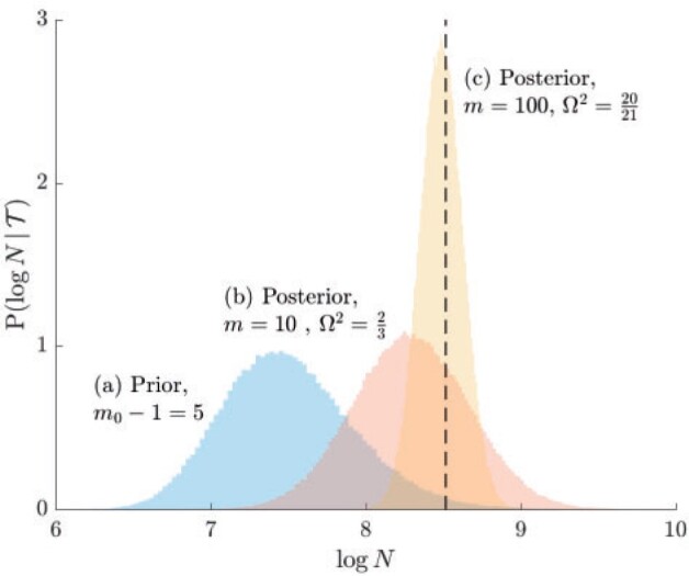
Effect of conjugate prior on Kingman coalescent estimation. We examine the relative impact on estimate precision of a conjugate Kingman prior that contributes virtual observations. We work in for convenience. We compare this prior to posteriors, which are obtained under observed trees with (red) and (yellow) coalescent events. The true value is in black. The prior contribution decays as increases towards 1.

Skyline Smoothing Priors

In this section, we tailor for the BSP, Skyride, and Skygrid coalescent inference methods. These popular skyline-based approaches couple a piecewise-constant demographic coalescent data likelihood with a smoothing prior to produce population size estimates that change more continuously with time. The smoothing prior achieves this by assuming informative relationships between and its neighboring parameters . Such a priori correlation implicitly introduces additional demographic information that is not available from the coalescent data . While these priors can embody sensible biological assumptions, we show that they may also engender overconfident statements or obscure parameter non-identifiability. We propose as a simple but meaningful analytic for diagnosing these problems.

We first define uniquely objective (i.e., uninformative) reference skyline priors, which we denote . Finding objective priors for multivariate statistical models is generally nontrivial, but (Berger et al., 2015) state that if has form then . Here, and are some functions and symbolizes the vector excluding . Following this, we obtain the objective priors

with , as normalization constants. Given its optimal properties (Parag and Pybus 2019), we only consider , and drop explicit notational references to it. Under this parametrization, and its expectation with respect to the prior are equal, that is . In addition, the reference prior in this case is , with as a matrix of zeros. This yields by Equation (4). A uniform prior over log-population space is hence uniquely objective for skyline inference.

Other prior distributions, which are subjective by this definition, necessarily introduce extra information and contribute to the posterior estimate precision. This contribution will result in . The two most widely used, subjective, skyline plot smoothing priors are:

• (i)the Sequential Markov Prior (SMP) used in the BSP (Drummond et al. 2005), and
• (ii)the Gaussian Markov Random Field (GMRF) prior employed in both the Skyride and Skygrid methods (Minin et al. 2008; Gill et al. 2013).

As the SMP and GMRF both propose nearest neighbor autocorrelations among elements of , tridiagonal posterior Fisher information matrices result. We represent these as and , respectively.

The SMP is defined as: (Drummond et al. 2005). It assumes that with a prior mean of . An objective prior is used for . To adapt this for , we define for . In the Appendix, we show how this expression yields Equation A1 and hence the transformed prior . We then take relevant derivatives to obtain , which for the minimally representative case is written as:

(10)

The matrices simply extend the tridiagonal pattern of Equation (10).

An issue with the SMP is its dependence on the unknown ``true'' demographic parameter values. As a result, we cannot evaluate (or control) a priori how much information is contributed by this smoothing prior. Rapidly declining populations could feature , for example, which would result in prior over-reliance. Conversely, exponentially growing populations would be more data-dependent. This likely reflects the asymmetry in using sequential exponential distributions. The only control we have on smoothing implicitly emerges from choosing the number of segments, . Some recent implementations of the BSP include an alternative log-normal prior that links with (Bouckaert et al. 2019), which is conceptually similar to the GMRF below.

The possibly strong or inflexible prior assumptions under the BSP motivated the development of the GMRF for the Skyride and Skygrid methods (Minin et al. 2008). The GMRF works directly with and models the autocorrelation between the neighbouring segments with multivariate Gaussian distributions. The GMRF prior (Minin et al. 2008) is defined as . In this model, is a normalization constant, a smoothing parameter, to which a gamma prior is often applied, and the values adjust for the duration of the piecewise-constant skyline segments. Usually, either (i) is chosen based on the inter-coalescent midpoints in or (ii) a uniform GMRF is assumed with for every .

Similarly, we calculate for the as:

(11)

The appendix provides the general derivation for any . As is arbitrary and the depend only on , the GMRF is insensitive to the unknown parameter values. This property makes it more desirable than the SMP and gives us some control (via ) of the level of smoothing introduced. Nevertheless, the next section demonstrates that this model still tends to over-smooth demographic estimates.

We diagonalize and to obtain matrices of form . Here is an orthogonal transformation matrix (i.e., ) and with as the eigenvalue of . Since , we can use Equation 4 to find that . This equality reveals that acts as a prior perturbed version of . When objective reference priors are used we recover and . We can use the matrix to gain insight into how the GMRF and SMP encode population size correlations. The principal components of our posterior demographic estimates (which are obtained from ) are the vectors forming the axes of the uncertainty ellipsoid described by .

These principal component vectors take the form when we apply the reference prior . Thus, as we would expect, our uncertainty ellipses are centered on the parameters we wish to infer. However, if we use the GMRF prior these axes are instead transformed to . These new axes are linear combinations of and elucidate how smoothing priors share information (i.e., introduce autocorrelations) about across its elements. These geometrical changes also hint at how smoothing priors influence the statistical properties of our coalescent inference problem.

To solidify these ideas, we provide a visualization of and an example of . We consider the simple case, where the posterior Fisher information and for the GMRF and SMP both take the form:

(12)

with for the GMRF and for the SMP. The signal-to-noise ratio is (see Equation 9), and performance clearly depends on how the coalescent events in are apportioned between the two population size segments.

We can lower bound the contribution of these priors to under any settings by using the robust coalescent design from (Parag and Pybus, 2019). This stipulates that we define our skyline segments such that in order to optimize estimate precision under . At this robust point, we also find that (or ) is attained. Figure 2 gives the uncertainty ellipses for this robust model at . These are constructed in coordinates centered about population size means as with controlling the confidence level.

Figure 2.

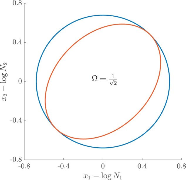
Uncertainty ellipses for SMP and GMRF. We show the improvement in asymptotic precision rendered by use of a smoothing prior for a segment skyline inference problem. The prior informed ellipse (red) is smaller in volume and has skewed principal axes relative to the purely data informed one (blue). All ellipses represent confidence with the indicating coordinate directions about their means, which are the log population sizes, . The covariance that smoothing introduces controls the skew of these ellipses. Here, , (total coalescent event count) and (this controls the prior influence see Equation 12). Larger values lead to over-reliance on the smoothing prior.

Here is either or . Because is diagonal the data-informed confidence ellipse has principal axes aligned with . The covariance among population size segments in , which is induced by the smoothing prior, skews these principal axes. We can see this by diagonalizing at and for every to obtain:

(13)

Applying , we find that the axes of our uncertainty ellipse (as visible in Figure 2) have changed from to . Sums and differences of log-populations are now the parameters that can be most naturally estimated under the SMP and GMRF. The reduction in the area of the ellipses of Figure 2 is a proxy for .

The Dangers of Smoothing

Having defined ratios for measuring the contribution of smoothing priors to the precision of estimates, we now use them to explore and expose the conditions under which prior over-reliance is likely to occur in practice. We assume that skyline segments are chosen to satisfy the robust design for (Parag and Pybus 2019), with as the total number of skyline segments. We previously proved that robust designs, at , minimize dependence on the prior (maximize ). While this is not the case for , in Figure A1 of the Appendix, we illustrate that the maximal point is generally well approximated by this robust setting. The values computed here are therefore conservative for most settings. Other experimental designs rely more on the prior.

As in Equation 5, we use the threshold to diagnose when the coalescent data (likelihood) and prior are equally influencing demographic posterior estimate precision. At the total Fisher information doubles since . We previously uncovered the importance of this threshold in the Kingman conjugate prior problem, where it signified an equality between the number of pseudo and real samples contributed by the prior and data, respectively. As (see Equation 8), this setting is also meaningful because it achieves a unit signal-to-noise ratio for any skyline-based model.

We first reconsider the case of Equation 12, where controls the prior contribution to . Here suggests , which implies that we are overly-reliant on smoothing when is larger than of the total observed coalescent events. This occurs when or , for the SMP and GMRF respectively. The improved precision due to the prior at this threshold is shown in Figure 2. The relative ellipse area (and hence ) will shrink further as we deviate from robust designs.

As the number of skyline segments, , increase, smoothing becomes more influential and can promote misleading conclusions. For the cases, we will only examine the GMRF, since the SMP has the undesirable property of dependence on the unknown values. To better expose the impact of the smoothing parameter , we will assume a uniform GMRF () so that then only depends on and . We compute and hence , at various . For example, we find that

under the robust design. Interestingly, the order of the polynomial dependence of (and hence ) on increases with . We find that this trend holds for any design. We will use the term robust for when is calculated under a robust design.

Figure 3 plots the robust against and for the uniform GMRF. A key feature of Figure 3 is the steep -dependent decay of relative to the threshold, which exposes how easily we can be unduly reliant on the prior, as increases. Given a phylogeny , increasing the complexity of a skyline-based model enhances the dependence of our posterior estimate precision on the smoothing prior. This pattern is intuitive as fewer coalescent events now inform each demographic parameter (Parag and Pybus 2019). However, decays with surprising speed. For example, at (the lowest curve in Figure 3), we get for and . Usually, has a gamma-prior with mean of 1 (Minin et al. 2008). We show the corresponding mutual information increases due to these GMRF priors in Figure A2 of the Appendix.

Figure 3.

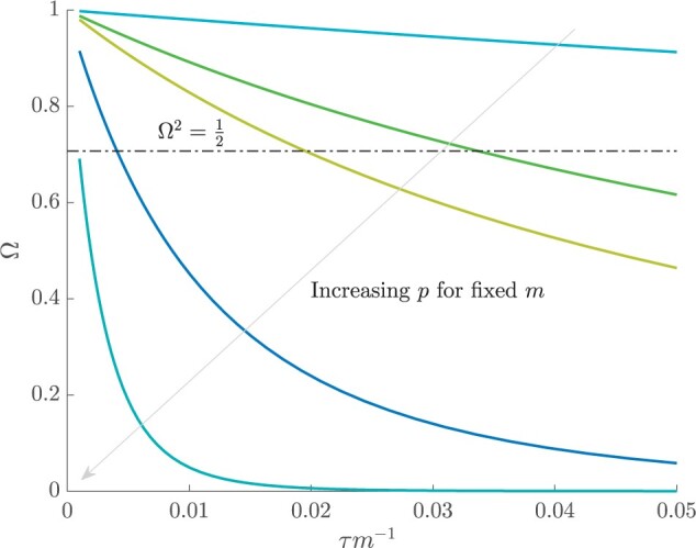
The impact of smoothing priors increases with skyline complexity. For the GMRF, we find that for a fixed (ratio of smoothing parameter to total coalescent event count), significantly depends on the complexity, , of our skyline. The colored curves are (along the arrow) for at with as the number of coalescent events per skyline segment. The dashed line depicts the threshold below which the prior contributes more than the coalescent data to posterior estimate precision (asymptotically). For a given tree and , the larger the number of demographic parameters we choose to estimate, the stronger the influence of the prior on those estimates.

While Figure 3 might seem specific to the uniform GMRF, it is broadly applicable to the BSP, Skyride, and Skygrid methods. We now outline the implications of Figure 3 for each of these skyline-based approaches.

(1) Bayesian Skyline Plot. This method uses the SMP, which depends on the unknown values. However, the results of Figure 3 remain valid if we set to , which results in the smallest non-data contribution to Equation 10. This follows as and have similar forms. While this choice underestimates the impact of the SMP, it still cautions against high- skylines and confirms suspected BSP issues related to poor estimation precision when skylines are too complex, or the coalescent data are not sufficiently informative (Ho and Shapiro 2011). However, good use of the BSP grouping parameter (Drummond et al. 2005), which sets , could alleviate these problems.

(2) Skyride. When this method uses the uniform GMRF, all results apply exactly. In its full implementation, the Skyride employs a time-aware GMRF that sets based on and estimates from the data (Minin et al. 2008). However, even with these adjustments, the GMRF can over-smooth, and fail to recover population size changes (Ho and Shapiro 2011; Faulkner et al. 2019). Our results provide a theoretical grounding for this observation. The Skyride constrains and then smooths this noisy piecewise model. Consequently, it constructs a skyline which is too complex by our measures (the lowest curve in Equation 3 is at ). By rescaling the smoothing parameter to , the curves in Figure 3 upper bound the true values of the time-aware GMRF.

(3) Skygrid. This method uses a scaled GMRF. For a tree with TMRCA , the Skygrid assumes new population size segments every time units (Gill et al. 2013). As a result, every and the time-aware GMRF becomes uniform with rescaled smoothing parameter . Therefore, the conclusions of Figure 3 hold exactly for the Skygrid, provided the horizontal axis is scaled by . This setup reduces the rate of decay but the curves still caution strongly against using skylines with . Unfortunately, as its default formulation sets to 1 less than the number of sampled taxa (or lineages) (Gill et al. 2013), the Skygrid is also be vulnerable to prior over-reliance.

The popular skyline-based coalescent inference methods therefore all tend to over-smooth, resulting in population size estimates that can be overconfident or misleading. This issue can be even more severe than Figure 3 suggests since in current practice is often close to and non-robust designs are generally employed. Further, skylines are only statistically identifiable if every segment has at least 1 coalescent event (Parag and Pybus 2019; Parag et al. 2020). Consequently, if is set, smoothing priors can even mask identifiability problems. We recommend that must be guaranteed and in the next section derive a model rejection guideline for finding , the suggested minimum number of coalescent events per skyline segment, and diagnosing prior over-reliance.

Prior Informed Model Rejection

We previously demonstrated how commonly-used smoothing priors can dominate the posterior estimate precision when coalescent inference involves complex, highly parametrized (large-) skyline models. Since data are more influential than the prior when , we can use this threshold to define a simple -rejection policy to guard against prior over-reliance. Assume that the matrix resulting from our prior of interest is symmetric and positive definite. This holds for the GMRF and SMP. The standard arithmetic–geometric mean inequality, , then applies with denoting the matrix trace. Since , we can expand this inequality and substitute in Equation 4 to get .

Since this inequality applies to all , we can maximize its right hand side to get a tighter lower bound on . This bound, termed , is achieved at the robust design and is given by

(14)

We define as a conservative model rejection criterion with implying that . If is the largest satisfying these inequalities (see Equation 14, indicates argument), then any skyline with more than segments is likely to be overly dependent on the prior and should be rejected under the current coalescent data or tree.

Alternatively, we recommend that skylines using a smoothing prior (with matrix ) should have at least events per segment to avoid prior reliance. The condition in Equation 14 ensures skyline identifiability (Parag and Pybus 2019) and generally (i.e., ). The dependence of on means that additions to the diagonals of necessarily increase the precision contribution from the prior. This insight supports our previous analysis, which used from the uniform GMRF to bound the performance of the SMP and time-aware GMRF. In the Appendix (see Equation A2) we derive analogous rejection bounds based on the excess mutual information, , from Equation 7. There we find that acts like an information-theoretic bandwidth, controlling the prior-contributed mutual information.

Equation 14, which forms a key contribution of this work, can be computed and is valid for any smoothing prior of interest. For the uniform GMRF where , we get . Note that here whenever or , as expected (i.e., there is no smoothing at these values). In Figure A4 of the Appendix, we confirm that is a good lower bound of . We enumerate across and , for an observed tree with , to get Figure 4, which recommends using no more than segments (). In Figure A5, we plot curves for various and , defining boundaries beyond which skyline estimates will be overly dependent on the GMRF.

Figure 4.

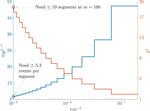
Bounding skyline complexity using the prior-data tradeoff. For the GMRF with uniform smoothing, we show how the maximum number of recommended skyline segments, (red), decreases with prior contribution (level of smoothing, i.e., increasing ). Hence the minimum recommended number of coalescent events per segment, (blue), rises. Here, we use the boundary (Figure 14), which approximates and provides a more easily computed measure of prior-data contributions. At larger the at a given decreases. The measure provides a model rejection tool, suggesting that models with should not be used, as they would risk being overly informed by the prior.

In the Appendix, we further analyze Equation 14 for the uniform GMRF to discover that is bounded by curves with exponents linear in and quadratic in (see Equation A3). This explains how the influence of smoothing increases with skyline complexity and yields a simple transformation , which can negate prior over-reliance. For comparison, the Skyride implements . The marked improvement, relative to Figure 3, is striking in Figure A3. Other revealing prior-specific insights can be obtained from Equation 14, reaffirming its importance as a model rejection statistic.

Our model rejection tool of Equation 14 can serve as a useful diagnostic for skyline over-parametrization, and as a precaution against prior over-reliance. However, we do not propose as the sole measure of optimal skyline complexity; because while warns against the prior being too relatively influential, it does not guarantee any absolute estimate precision. For example, a small pair might produce the same as a larger pair. Choosing an optimal in a data-justified manner is an open problem that is still under active study (Parag and Donnelly 2020). We next illustrate how , via its more easily computed approximation, , can be practically applied to detect and reject over-smoothed skyline plot models, using data sets that are commonly employed to evaluate the performance of coalescent demographic inference.

Illustrative Examples: Egyptian HCV and Beringian Bison

We validate the practical utility of (and hence ), as a diagnostic of prior over-dependence, by investigating changes in effective population size inferred from the well-studied Egyptian HCV-4 (Pybus et al. 2003) and Beringian steppe bison (Shapiro et al. 2004) data sets. The first consists of 63 partial sequences of HCV genotype 4 and was previously analyzed in (Pybus et al., 2003) using a coalescent model with a parametric demographic function that featured periods of constant population size separated by a phase of exponential growth. The second data set comprises 152 modern and partial mtDNA and was investigated in (Shapiro et al., 2004), where skyline plot models confirmed a demographic history of exponential growth then decline (boom-bust) with an additional bottleneck dynamic (Drummond et al. 2005). These two data sets have since been re-examined under various alternate models in (Minin et al., 2008), (Gill et al., 2013), (Parag et al., 2020) and several other studies.

We simulated 100 trees with and tips, using the software package MASTER (Vaughan and Drummond 2013), according to inferred HCV and bison population size trends, respectively. The HCV population size trend that we simulated from is provided in (Pybus et al., 2003). We inferred the population size trend of the bison data set using the BSP (with sequential Markovian prior) in accordance with published analyses (Drummond et al. 2005). We used 20 population groups and the optimal design from (Parag and Pybus 2019) to ensure that we captured complex bison population dynamics reliably. As our focus is on exploring the behavior of skylines and given a particular underlying population size trend and not the uncertainty associated with that trend, we used the posterior mean (HCV) or median (bison) of these inferred trends for simulating trees and do not consider genealogical uncertainty.

The simulated set of coalescent trees from each data set provide an approximate measure of the coalescent variance that could arise from the inferred underlying population size trends. We then estimated from every simulated tree using various skyline models with time-aware GMRF smoothing priors, as in (Minin et al., 2008). We varied the relative contributions of the coalescent data and GMRF to our posterior log-population size estimates by changing either the skyline dimension, , or the GMRF smoothing parameter . As is fixed for a given data set and robust designs are applied, increasing the number of coalescent events in each segment, , reduces .

We analyzed every tree over all combinations of across a wide range of . For comparison, we also generated purely data-informed estimates of , for the same , by replacing the subjective GMRF with a uniform, objective prior. We computed from Equation 14 for these settings in Figure 5 and observe that, as expected, it decreases with both and (i.e., increases with ). Practical analyses of these data sets using Skyride or Skygrid approaches, would choose or infer a value and set . However, Figure 5 shows and hence events per skyline parameter are often necessary to achieve . This raises questions about the validity of the common practice of applying these methods using their default settings.

Figure 5.

Model rejection statistics for the HCV and bison data sets The metric is calculated for each tree (see Equation 14) under a time-aware GMRF for various combinations of its smoothing parameter and , the number of coalescent events per skyline segment. The box-plots summarize the resulting over 100 simulated trees that represent the demographic histories of the (A) Egyptian HCV and (B) Beringian bison data sets. The solid lines link the median values across boxes for a given and hence skyline dimension (). We discourage the use of skyline models with .

Figure 5 confirms that the recommended maximum skyline dimension falls and hence the minimum allowable number of coalescent events per segment grows as the smoothing parameter increases. We demonstrate the qualitative difference in skyline-based estimates between values on either side of the criterion for a single simulated HCV and bison tree in Figure 6. In panels A and C, we present the Skyride estimate, which uses and implements , at the chosen values (0.05 and 1). Contrastingly, in B and D, we illustrate an equivalent skyline with a different , which achieves at this same , according to our metric (see the and curves at and in panels A and B of Figure 5, respectively). We overlay the corresponding skyline (with the same ) obtained with an objective uniform prior, to visualize the uncertainty engendered from the coalescent data alone.

Figure 6.

HCV and bison demographic estimates under GMRF and uniform priors. We analyze demographic estimates under time-aware GMRF priors (blue) and objective uniform priors (red) for a single tree simulated under the demographic scenarios inferred from the Egyptian HCV (A) and (B) and Beringian bison (C) and (D) data sets. In (A) and (C), we present Skyride estimates, which use and (A) and (C). These skylines have dimension that is larger than our maximum recommended dimension , which is computed from Figure 5. In (B) and (D), we re-estimate population size at (B) and (D). These groupings of coalescent events achieve as justified by our metric (see Equation 14). Solid lines are posterior medians while semi- transparent blocks are the 95% HPD intervals.

At (panels A and C of Figure 6), the uniform prior produces a skyline that infers more rapid demographic fluctuations through time than that estimated with the GMRF prior. Further, the 95% HPD intervals from the uniform prior (red) are substantially wider than those from the GMRF prior (blue) in both examples, highlighting the marked contribution of the time-aware GMRF prior to posterior estimate precision. While this smoothed trajectory looks reliable we argue that, because (and hence ), it is difficult to justify using the data alone and that the prior is responsible for too much of the estimate precision. In contrast, at and (panels B and D of Figure 6), which apply , both prior distributions yield more similar skylines, implying that GMRF smoothing has not substantially inflated posterior estimate precision.

Under these settings, we have fewer demographic fluctuations than for because 4 and 2 times more coalescent events are informing each parameter or skyline segment, respectively. We achieve smaller uncertainty than with a uniform prior (which is overfitted) but without excessively relying on the GMRF smoothing, which at is likely underfitting. The metric and hence criterion help us better balance data, noise, and our prior assumptions. In contextualizing these results it is important to note that skyline plots provide harmonic mean and not point estimates of population size (Pybus et al. 2000). Consequently, we are inferring sequences of means from our coalescent data, which a priori may not need to conform to a smooth pattern.

The HCV example shows that for times beyond years there are so few events that it is more sensible to estimate a single mean (panel B), which we are confident in across this period, as opposed to several less certain and overfitted means (panel A). In contrast, for the bison example, the bottleneck over years is over-smoothed (panel C), despite many coalescent events occurring in that region. The simple correction of extending our harmonic mean over 2 events (panel D) restores the necessary fall in population size. Deciding on how to balance uncertainty with model complexity is non-trivial and, as shown in these examples, caution is needed to avoid misleading conclusions. We posit that (and hence ) can help formalize this decision-making and improve our quantification of the uncertainty across skyline plots.

Having confirmed as a credible measure of relative uncertainty, we briefly explore how it relates to more easily ascertained measures of uncertainty. For each simulated coalescent tree in the HCV example above, we computed (via Equation 4) and two ancillary statistics based on the 95% highest posterior density (HPD) intervals of the estimates. These are the median HPD ratio and the relative HPD product (across the skyline segments) , which are formulated as:

with med indicating the median value of a set. Here is the 95% HPD interval of under a GMRF with smoothing parameter and is the equivalent HPD when the objective uniform prior is applied instead.

The 95% HPD interval is closely connected to the inverse of the Fisher information matrices that define and, further, describes the most visually conspicuous representation of the uncertainty present in skyline plot estimates. Comparing to these ancillary statistics, which evaluate the median and total 95% uncertainty of a skyline plot, allows us to contextualize against more relatable (though different) and obvious visualizations of posterior performance. We present these comparisons in Figure A6 of the Appendix. There we find that all statistics monotonically decay with that is as the time-aware GMRF becomes more informative. The sharpness of this decay is highly sensitive to . Larger means that more coalescent data are informing each estimated parameter (smaller ).

The reduced decay with supports our assertion that acts as an exponent controlling prior over-reliance (see Fig. 3). The gentler decay of (relative to and ), which largely does not account for , confirms that we could be misled in our understanding of the impact of smoothing if we neglected skyline dimension. In contrast and , which both measure, in some sense, the relative volumes of uncertainty across the entire skyline-plot due to the data alone and the data and prior, fall more significantly and consistently. At (), which is the most common setting in the Skyride and Skygrid methods, both statistics are markedly below and posterior estimates will often be too dependent on the prior. This high- behavior is also indicative of model overparametrization (Parag and Donnelly, 2020). Our metric therefore relates sensibly to visible and common proxies of uncertainty.

Discussion

Popular approaches to coalescent inference, such as the BSP, Skyride, and Skygrid methods, all rely on combining a piecewise-constant population size likelihood function with prior assumptions that enforce continuity. This combination, which is meant to maximize descriptive flexibility without sacrificing the smoothness that is expected to be exhibited by real population size curves over time, has led to many insights in phylodynamics (Ho and Shapiro 2011). However, it has also spawned concerns related to over-smoothing and lack of methodological transparency (Minin et al. 2008; Faulkner et al. 2019). In this work, we attempted to address these concerns by deriving metrics for diagnosing and clarifying the existing assumptions present in current best practice.

Detecting and correcting for underfitting or over-smoothing is crucial if reliable and meaningful assessments of the effective population size changes of a species or pathogen of interest are to be made from sequence data. Abrupt changes in effective population size are not only biologically plausible but may also signal key events that have shaped the demographic histories of populations (Pyron and Burbink 2013). In ecology, identifying rapid extinctions and bottlenecks in diversity might signify the impact of environmental change or anthropogenic influences (e.g., hunting or changes in land use) (Stiller et al. 2010; Thomas et al. 2019). Similarly, in epidemiology, sharp fluctuations in the prevalence of an infection might support hypotheses about emergence in novel populations, seasonality, the effect of interventions, vaccines, or drug treatments. Further, rapid exponential growth of any population may, when observed over a longer timescale, appear as a near-stepwise transition in population size.

Underfitting or over-smoothing these changes would limit understanding of the dynamics of the study population and could affect conclusions about the potential causative factors that influenced those dynamics. However, recognizing when commonly used methods for inferring these demographic trends are over-smoothing is difficult. By capitalizing on (mutual) information theory and (Fisher) information geometry, we formulated the novel coalescent information ratio, , which provides a rigorous means of solving this over-smoothing problem. This ratio describes both the proportion of the asymptotic uncertainty around our posterior estimates that is due solely to the data and the additional mutual information that the prior assumptions introduce.

We derived analytic expressions for for the BSP, Skyride, and Skygrid estimators of effective population size, which combine piecewise skyline likelihoods with either SMP or GMRF smoothing priors. We also showed that has an exact and intuitive interpretation as the ratio of real coalescent events to the sum of real and virtual (prior-contributed) ones in a Kingman coalescent model. Using as a threshold delimiting when the prior contributes as much information as the coalescent data, we found that it is easy to become overly dependent on prior assumptions as the skyline dimension, , increases (for a fixed tree size). This central result emerges from the drastic reduction in the number of coalescent events informing on any population size parameter as rises. Per parameter, the BSP and Skyride use only a few or one event respectively (Minin et al. 2008; Drummond et al. 2005), while the Skygrid may have no events informing some parameters (Gill et al. 2013).

These issues can be obscured by current Bayesian implementations, which can still produce apparently reasonable population size estimates, at least visually, as illustrated in our simulated HCV and bison case studies. Our simulations indicate that analyses that combine maximally parametrized skylines (one event per segment or parameter) with GMRF smoothing can lead to errors in population size inference. For trees simulated according to the HCV demographic scenario, estimates were likely overfitted in the far past, inflating HPDs, but over-smoothed towards the present. The resulting skyline uncertainty contrasted that from the original (Pybus et al. 2003) and later (Parag and Pybus 2017) analyses. In the bison example, we found evidence for underfitting. The inferred skyline there emphasized a smoother boom-bust trend with concentrated HPDs. However, this underestimated the depth of a bottleneck during which coalescent events were concentrated.

These mismatches between data and smoothing can be difficult to diagnose and problematic, not just for prior over-dependence. Low coalescent event counts, for example, can lead to poor statistical identifiability (Rothenburg 1971), which might manifest in spurious MCMC mixing. Consequently, we proposed a practical rejection criterion for ensuring that coalescent data is the main source of inferential information. This criterion, which was based on an approximation to , provided a way of regularizing skyline complexity. When applied to our examples it recommended a 4-event skyline grouping that resulted in demographic reconstructions that were more consistent with the above mentioned HCV studies. It also suggested a simple 2-event grouping that recovered the bison bottleneck dynamic without generating too much estimate noise.

This criterion bounds the maximum recommended skyline dimension for a given data set (tree) size and provides a usable means of defining the minimum number of coalescent events, , which we should allocate to each skyline segment to guard against too much prior influence. Since only requires our computing the sum of the diagonals of the prior Fisher matrix, it can serve as a simple rule-of-thumb for sensibly balancing the prior-data tradeoff in skyline plots (e.g., in the BSP, the grouping parameter might be set to a value above to ensure well-regularized estimates). As we found to be lower-bounded by more visible measures of skyline uncertainty, such as the product of relative HPD widths, useful approximations to and may also be computed from these measures.

Our metric also provides insight into how we can alleviate the dramatic impact of skyline complexity on prior over-reliance. When specialized to the GMRF, for example, it reveals that we can negate over-smoothing by scaling the smoothing parameter with a quadratic of . Moreover, it shows that only by increasing the information available from the sampled phylogeny can we reasonably allow for more complex piecewise-constant functions under a given prior. Recent methods, such as the epoch sampling skyline plot (Parag et al. 2020), which can double the Fisher information extracted from a given phylogeny by exploiting the informativeness of sampling times, would support higher dimensional skylines. Such approaches have the potential to increase the contribution of the data without elevating the influence of the smoothing prior.

While in this article we have applied to non-parametric, skyline inference problems in population genetics, ecology and infectious disease epidemiology, its general formulation in Equation 4 is more widely applicable. It can be also applied to coalescent inference problems where specific parametric models (e.g., exponential/logistic growth) are used, in order to disentangle the contributions of observed data and the prior distributions over these parameters, though numerical solutions will likely be necessary. More generally, our approach is valid for any statistical problem, provided the Hessian matrices necessary for deriving the prior and data Fisher information terms are valid and computable. This is not limited to prior-data tradeoffs. Similar ratio metrics should be derivable by comparing Fisher information terms from different sources (e.g., to test whether one source of data is more informative than another).

Thus, we have devised and validated a rigorous means of better understanding, diagnosing and preventing prior over-dependence. We hope that our statistic, which clarifies and quantifies the often inscrutable impact of the prior and data, will help researchers make more active and considered design decisions when adapting popular skyline-based techniques. Our work also aligns with recent studies, which have started to re-examine both model selection and prior definition (Parag and Donnelly 2020; Faulkner et al. 2019) in an attempt to derive more reliable effective population size estimates from coalescent trees. While we believe that data-driven conclusions are generally the most justifiable we note that, in the context of skyline plots, this can be open to interpretation and the choice of prior is far from trivial.

Appendix

Smoothing Prior Fisher Information Matrices

Here, we derive the prior-informed Fisher information matrices for the SMP and GMRF smoothing priors. We start by finding the log-population size transformed version of the SMP smoothing prior. We then calculate its Hessian to get , and so obtain the general form of Equation 10. The SMP is given in (Drummond et al., 2005) as . We define so that its inverse . These expressions are in vector form so . We want the transformed prior . Applying the multivariate change of variables formula gives , with as the Jacobian of . This implies that . Substituting gives the SMP log-prior:

(A1)

We can then obtain , with . The diagonals of are: for , and . The non-zero off-diagonal terms are: and . The result is a symmetric tridiagonal matrix that has zero row and column sums. The matrix is then added to the Fisher information matrix (with as the number of coalescent events informing on the parameter), to get .

We now compute , which is given in the main text as Equation (11). For the GMRF (Minin et al. 2008) and so . Taking second derivatives we get diagonal terms of the Hessian, , as: for , and . The nonzero off diagonal terms are: and . The GMRF also gives a symmetric tridiagonal with row and column sums of zero. Adding to the diagonal matrix yields .

Further Smoothing Results

In the main text, we asserted that the computed at the robust point of (Parag and Pybus 2019) generally upper bounds the achievable values at other settings. Here we provide evidence for this assertion. While strictly (except for ), we numerically find that . We show this for the GMRF under uniform smoothing in Figure A1. This makes sense as while (for fixed smoothing parameters) and , there is no reason to believe that this also maximizes their ratio. The sawtooth curves in Figure A1 reflect changes in the other values, given a fixed .

Hence, we used the robust design point in our calculation of the curves for the GMRF in Figure 3. The corresponding additional mutual information () curves for this case are provided in Figure A2. These show how larger values of the smoothing parameter, , directly lead to increases in the relative mutual information contribution from the prior. Observe that is highly sensitive to the skyline complexity, , thus clarifying how estimates from overparametrized skyline plots can be dominated by prior information.

Interestingly, we can largely negate the impact of skyline complexity by making a function of . In the main text we explained how the Skyride implicitly implements the scaling . While this reduces some of the effect of shown in Figure 3, it still leads to decaying curves that can, for a given , be deceptively dependent on smoothing. Here we propose the key transformation , as a means of reducing our smoothing in line with our skyline complexity. This transformation was inspired by the dependence of a lower bound on , which we derive in Equation A3 later in the Appendix. Its striking impact on the spread of curves from Figure 3 is given in Figure A3.

Figure A1.

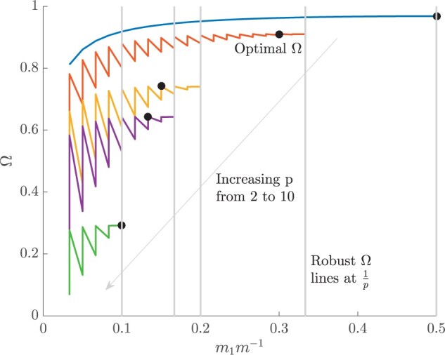
Robust and optimal designs. For the GMRF smoothing prior with for all and , we show that the optimal design point is not always the same as the robust design point, at which . The colored curves are (along the dashed arrow) for at , and computed across all partitions for any given (hence the zig-zagged form). The gray vertical lines mark the robust point for each curve, and the black circles give the optimal points. While these lines and circles do not always match, both generally feature approximately the same values. We found this to be the case across several and values.

Figure A2.

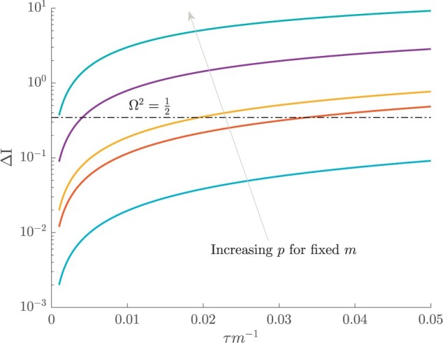
Prior mutual information increases with skyline complexity.} For the uniform GMRF, we show that under fixed smoothing (and hence ), the additional mutual information introduced by the prior, , significantly increases with the complexity, , of our skyline. The colored curves are (along the grey arrow) for at with (robust design point). The dashed   is also given for comparison. Clearly, the more skyline segments we have for a given tree, the more likely we are being overly informed by our prior.

Figure A3.

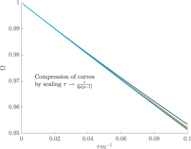
Negating the impact of skyline dimension. We show how an appropriate quadratic scaling of the GMRF precision parameter, , can remove the complexity () induced smoothing contribution portrayed in Figure 3 of the main text. This scaling significantly compresses the colored curves shown, which are for at with (robust design point). The resulting values are now all comfortably above the threshold and justified by our information theoretic metrics.

Further Model Selection Bounds

In the the main text, we derived lower bounds on , which led to the model rejection parameter, (see Equation 14). Here, we extend and support those results. In Figure A4, we first show that the bound of Equation 14 is a good measure of the true value, for a skyline with uniform GMRF smoothing. We used this bound to define a maximum , , above which the skyline would be over-parametrized and susceptible to prior induced overconfidence. We explore over and for this GMRF in Figure A5 and observe that becomes more restrictive with fewer observed data (coalescent events) or increased smoothing. This supports as a useful measure of prior-data contribution.

Figure A4.

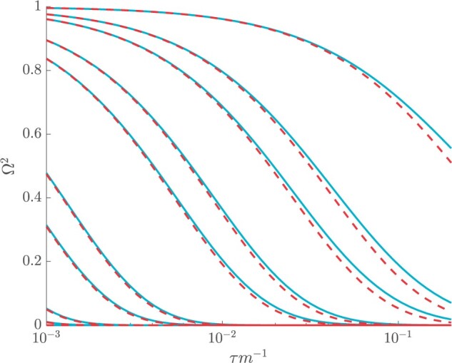
Lower bounds on . For the GMRF smoothing prior with for all and , we compare the lower bound on (red, dashed, see Equation 14) with the actual value of (cyan) at the robust design point of . We examine all integer values that are factors of , and find that qualitatively similar comparisons hold for different and settings. In general the lower bound () is a good approximation to .

Figure A5.

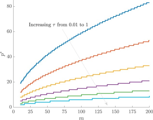
Maximum model selection boundary. For the GMRF smoothing prior with for all and at the robust point , we compute the maximum allowed number of skyline segments, , such that . These curves increase with and decrease with , indicating how the prior-data contribution can be used to define model rejection regions. Skylines with would be overly informed by the prior and hence should not be used.

Figure A6.

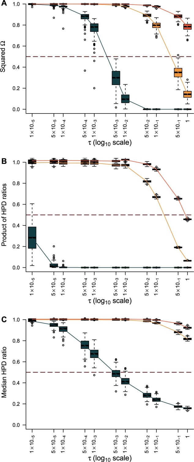
Trends in HPD-based statistics and under various time-aware GMRF settings. The (panel A), median HPD ratio of (panel B) and HPD product (panel C) statistics are computed across over various combinations of and . Box-plots summarize our results over 100 observed coalescent trees simulated from previously inferred demographic trends found for the Egyptian HCV data set. Analyses with are in dark green, in yellow and in orange. The solid lines link the median values across boxes for a given value. The dashed line is positioned at the threshold .

Lower bounds on imply upper bounds on the excess mutual information, (see Equation 7). We manipulate Equation 14 (under a robust design) to obtain the first inequality in Equation A2, with as follows

(A2)

This expression reveals that is akin to a signal bandwidth, by comparison with standard Shannon–Hartley theory (Cover and Thomas 2006) and is therefore a key controlling factor in defining how much additional information the prior will introduce. This supports our proposed rejection criterion.

Under the parametrization, and are symmetric, positive definite matrices. For such matrices we can apply a theorem from (Huang and Zhang, 2018), which states that , with . At the robust point, we get , which leads to the second inequality in Equation A2. Thus, our bound is tighter than that in (Huang and Zhang, 2018), and useful for broader, future mathematical analyses of . This inequality also clarifies why is often important for characterizing performance here.

We can also use the bound of (Huang and Zhang, 2018) to derive alternate (but slacker) lower bounds on . This gives the first inequality in Equation A3. Applying this to the uniform GMRF gives the second inequality:

(A3)

Interestingly, Equation A3 shows that the dependence of on the smoothing parameter is at most only linear, while the dependence on complexity can be quadratic. This provides further theoretical backing for the use of to reject models and emphasizes how smoothing can play a deceptively prominent role in the resulting estimate precision produced under complex (high-dimensional) skyline plots.

Ancillary Uncertainty Statistics

In the Egyptian-HCV simulated example, we defined two 95% HPD based ancillary statistics for characterizing the visual uncertainty present in a skyline plot demographic estimate. In Figure A6, we plot these statistics and for various and values under a time-aware GMRF. We discuss the implications of Figure A6 in the main text but observe here that trends between the more common (and more easily visualized) HPD based measures and our novel statistic are largely consistent.

Funding

This study was funded by the UK Medical Research Council (MRC) and the UK Department for International Development (DFID) under the MRC/DFID Concordat agreement and is also part of the EDCTP2 programme supported by the European Union [grant reference MR/R015600/1]. This work was also supported by the Oxford Martin School.

Supplementary Material

Data available from the Dryad Digital Repository: https://datadryad.org/stash/dataset/doi:10.5061/dryad.1jwstqjs2.

References

- Beerli P., Felsenstein J. 1999. Maximum likelihood estimation of migration rates and effective population numbers in two populations using a coalescent approach. Genetics 152:763–773. [DOI] [PMC free article] [PubMed] [Google Scholar]
- Ben-Haim Z., Eldar Y. 2009. A lower bound on the Bayesian MSE based on the optimal bias function. IEEE Trans. Information Theory 55(11):5179–5196. [Google Scholar]
- Berger J., Bernardo J., Sun D. 2015. Overall objective priors. Bayesian Anal. 10(1):189–221. [Google Scholar]
- Bouckaert R., Vaughan T., Barido-Sottani J., Duchêne S., Fourment M., Gavryushkina A., Heled J., Jones G., Kühnert D., De Maio N., Matschiner M., Mendes F., Müller N., Ogilvie H., du Plessis L., Popinga A., Rambaut A., Rasmussen D., Siveroni I., Suchard M., Wu C., Xie D., Zhang C., Stadler T., Drummond A. 2019. BEAST 2.5: an advanced software platform for Bayesian evolutionary analysis. PLoS Comput. Biol. 15(4):e1006650. [DOI] [PMC free article] [PubMed] [Google Scholar]
- Brunel N., Nadal J. 1998. Mutual information, fisher information, and population coding. Neural Comput. 10:1731–1757. [DOI] [PubMed] [Google Scholar]
- Cover T., Thomas J. 2006. Elements of information theory. 2nd ed. New Jersey: Wiley. [Google Scholar]
- Drummond A., Nicholls G., Rodrigo A., Solomon W. 2002. Estimating mutation parameters, population history and genealogy simultaneously from temporally spaced sequence data. Genetics 161:1307-1320. [DOI] [PMC free article] [PubMed] [Google Scholar]
- Drummond A., Rambaut A., Shapiro B., Pybus O. 2005. Bayesian coalescent inference of past population dynamics from molecular sequences. Mol. Biol. Evol. 22:1185-1192. [DOI] [PubMed] [Google Scholar]
- Faulkner J., Magee A., Shapiro B., Minin V. 2019. Horseshoe-based Bayesian nonparametric estimation of effective population size trajectories. Biometrics. 76:677–690. [DOI] [PubMed] [Google Scholar]
- Fink D. 1997. A compendium of conjugate priors. Technical Report, Montana State University. [Google Scholar]
- Gill M., Lemey P., Faria, N., Rambaut A., Shapiro B., Suchard M. 2013. Improving Bayesian population dynamics inference: a coalescent-based model for multiple loci. Mol. Biol. Evol. 30(3):713–724. [DOI] [PMC free article] [PubMed] [Google Scholar]
- Griffiths R., Tavare, S. 1994. Sampling theory for neutral alleles in a varying environment. Philos. Trans. R. Soc. B 344:403–410. [DOI] [PubMed] [Google Scholar]
- Ho S., Shapiro B. 2011. Skyline-plot methods for estimating demographic history from nucleotide sequences. Mol. Ecol. Resour. 11:423–434. [DOI] [PubMed] [Google Scholar]
- Huang W., Zhang K. 2018. Information-theoretic bounds and approximations in neural population coding. Neural Comput. 30(4):885–944. [DOI] [PMC free article] [PubMed] [Google Scholar]
- Ipsen I., Rehman R. 2008. Perturbation bounds for determinants and characteristic polynomials. SIAM J. Matrix Anal. Appl. 30(2):762–776. [Google Scholar]
- Kingman J. 1982. On the genealogy of large populations. J. Appl. Probab. 19:27–43. [Google Scholar]
- Kuhner M., Yamato J., Felsenstein J. 1998. Maximum likelihood estimation of population growth rates based on the coalescent. Genetics 149:429–434. [DOI] [PMC free article] [PubMed] [Google Scholar]
- Lehmann E., Casella G. 1998. Theory of point estimation. 2nd ed. New York:Springer. [Google Scholar]
- Li H., Durbin R. 2011. Inference of human population history from individual whole-genome sequences. Nature 475(7357): 493-496. [DOI] [PMC free article] [PubMed] [Google Scholar]
- Minin V., Bloomquist E., Suchard M. 2008. Smooth Skyride through a rough Skyline: Bayesian coalescent-based inference of population dynamics. Mol. Biol. Evol. 25(7):1459–1471. [DOI] [PMC free article] [PubMed] [Google Scholar]
- Parag K., Donnelly C. 2020. Adaptive estimation for epidemic renewal and phylogenetic Skyline models. Syst. Biol. 69(6):1163–1179. [DOI] [PMC free article] [PubMed] [Google Scholar]
- Parag K., Pybus O. 2017. Optimal point process filtering and estimation of the Coalescent process. J. Theor. Biol. 421:153–167. [DOI] [PubMed] [Google Scholar]
- Parag K., Pybus O. 2019. Robust design for coalescent model inference. Syst. Biol. 68(5):730–743. [DOI] [PubMed] [Google Scholar]
- Parag K., du Plessis L., Pybus O. 2020. Jointly inferring the dynamics of population size and sampling intensity from molecular sequences. Mol. Biol. Evol. 37(8):2414–2429. [DOI] [PMC free article] [PubMed] [Google Scholar]
- Pybus O., Rambaut A., Harvey P. 2000. An integrated framework for the inference of viral population history from reconstructed genealogies. Genetics 155:1429–1437. [DOI] [PMC free article] [PubMed] [Google Scholar]
- Pybus O., Drummond A., Nakano T., Robertson B., Rambaut. A. 2003. The epidemiology and iatrogenic transmission of hepatitis C virus in Egypt: a Bayesian coalescent approach. Mol. Biol. Evol. 20(3):381–387. [DOI] [PubMed] [Google Scholar]
- Pyron R., Burbink F. 2013. Phylogenetic estimates of speciation and extinction rates for testing ecological and evolutionary hypotheses. Trends Ecol. Evol. 28(12):729–736. [DOI] [PubMed] [Google Scholar]
- Robert C. 2007. The Bayesian choice. Newyork:Springer Science and Business Media. [Google Scholar]
- Rodrigo A., Felsenstein J. 1999. Coalescent approaches to HIV-1 population. The evolution of HIV. Baltimore:Johns Hopkins University Press. [Google Scholar]
- Rothenburg T. 1971. Identification in parametric models. Econometrica 39(3):577–591. [Google Scholar]
- Shapiro B., Drummond A., Rambaut A., Wilson M., Matheus P., Sher A., Pybus O., Gilbert M., Barnes I., Binladen J., Willerslev E., Hansen A., Baryshnikov G., Burns J., Davydov S., Driver J., Froese D., Harington C., Keddie G., Kosintsev P., Kunz M., Martin L., Stephenson R., Storer J., Tedford R., Zimov S., Cooper A. 2004. Rise and fall of the Beringian steppe bison. Science 306(5701):1561–1565. [DOI] [PubMed] [Google Scholar]
- Slate E. 1994. Parameterizations for natural exponential families with quadratic variance functions. J. Am. Stat. Assoc. 89(428): 1471–1481. [Google Scholar]
- Snyder D., Miller M. 1991. Random point processes in time and space. 2nd ed. Newyork:Springer. [Google Scholar]
- Stiller M., Baryshnikov G., Bocherens H., d’Anglade A., Hilpert B., Munzel S., Pinhasi R., Rabeder G., Rosendahl W., Trinkaus E., Hofreiter M., Knapp M. 2010. Withering away-25,000 years of genetic decline preceded cave bear extinction. Mol. Biol. Evol. 27(5): 975–978. [DOI] [PubMed] [Google Scholar]
- Strimmer K., Pybus O. 2001. Exploring the demographic history of DNA sequences using the generalized skyline plot. Mol. Biol. Evol. 18(12):2298–2305. [DOI] [PubMed] [Google Scholar]
- Thomas J., Carvalho G., Haile J., Rawlence N., Martin M., Ho S., Sigfusson A., Josefsson V., Frederiksen M., Linnebjerg J., Castruita J., Niemann J., Sinding M., Sandoval-Velasco M., Soares A., Lacy R., Barilaro C., Best J., Brandis D., Cavallo C., Elorza M., Garrett K., Groot M., Johansson F., Lifjeld J., Nilson G., Serjeanston D., Sweet P., Fuller E., Hufthammer A., Meldgaard M., Fjeldsa J., Shapiro B., Hofreiter M., Stewart J., Gilbert M., Knapp M. (2019). Demographic reconstruction from ancient DNA supports rapid extinction of the great auk. eLife 8:e47509. [DOI] [PMC free article] [PubMed] [Google Scholar]
- Tichavsky P., Muravchik C., Nehorai A. 1998. Posterior Cramer-Rao bounds for discrete-time nonlinear filtering. IEEE Trans. Signal Process. 46(5):1386–1395. [Google Scholar]
- van Trees H. 1968. Detection, estimation, and modulation theory, Part I. New Jersey:Wiley. [Google Scholar]
- Vaughan T., Drummond A. 2013. A stochastic simulator of birth–death master equations with application to phylodynamics. Mol. Biol. Evol. 30(6):1480–1493. [DOI] [PMC free article] [PubMed] [Google Scholar]
- Wakeley J. 2008. Coalescent theory: an introduction. Colorado:Roberts and Company Publishers. [Google Scholar]