A Method for Estimating the Deposition Density of Fallout on the Ground and on Vegetation from a Low-yield, Low-altitude Nuclear Detonation

Abstract

This paper describes a relatively simple model developed from observations of local fallout from US and USSR nuclear tests that allows reasonable estimates to be made of the deposition density (activity per unit area) on both the ground and on vegetation for each radionuclide of interest produced in a nuclear fission detonation as a function of location and time after the explosion. In addition to accounting for decay rate and in-growth of radionuclides, the model accounts for the fractionation (modification of the relative activity of various fission and activation products in fallout relative to that produced in the explosion) that results from differences in the condensation temperatures of the various fission and activation products produced in the explosion. The proposed methodology can be used to estimate the deposition density of all fallout radionuclides produced in a low yield, low altitude fission detonation that contribute significantly to dose. The method requires only data from post-detonation measurements of exposure rate (or beta or a specific nuclide activity) and fallout time-of-arrival. These deposition-density estimates allow retrospective as well as rapid prospective estimates to be made of both external and internal radiation exposure to downwind populations living within a few hundred kilometers of ground zero, as described in the companion papers in this volume.

INTRODUCTION

Estimating the radiation health impact on an exposed population from a nuclear fission event requires a knowledge of the external radiation dose and the internal radiation dose from ingestion and/or inhalation. Estimated deposition densities (activity per area, i.e., Bq m⁻²) of each of the large number of radionuclides produced in the explosion provide the basis for subsequent estimates of organ doses from both external and internal exposure. This paper describes a relatively simple model developed from observations of local fallout from US and USSR nuclear tests that allows reasonable estimates to be made of the deposition density on both the ground and on vegetation for each radionuclide of interest produced in a nuclear fission event as a function of location and time after the explosion. In addition to accounting for decay rate and in-growth of radionuclides, the model accounts for the fractionation (modification of the relative activity of various fission and activation products in fallout relative to that produced in the explosion) that results from differences in the condensation temperatures of the various fission and activation products produced in the explosion.

The proposed methodology can be used to estimate the deposition density of each of the many fallout radionuclides that contribute significantly to radiation dose produced from a low yield, low altitude⁸ fission event. The method requires only data from post-detonation measurements of exposure rate coupled with the estimated fallout time-of-arrival (TOA). This allows relatively rapid prospective estimates of both external and internal radiation exposure to downwind populations living within a few hundred kilometers of ground zero (GZ). The modeled doses are based on the assumption of an absence of remediation activities that, of course, could modify the exposure rate. The model-deposition densities described in this paper are intended for use in estimating dose as described in the companion papers in this volume (Simon et al. 2022; Bouville et al. 2022; Anspaugh et al. 2022).

Although a number of complex computer models have been developed to predict the transport and deposition of nuclear debris, they require very accurate and precise meteorological data downwind and at the site of the detonation as well as specific information regarding the type of fissionable material and device composition and the distribution of activity particle-sizes in the debris cloud. Even if accurate meteorological data are available at the site of the explosion, there is often little data at downwind locations and, thus, accuracy tends to degrade as one moves further downwind. Furthermore, the type of fissile material in the device will usually not be initially known. The models described here require only a set of post-detonation exposure rate measurements and TOA estimates downwind.

The proposed model combines both US and Russian experience and strategies for modeling deposition and interception of fallout by vegetation in a framework that is suitable not only for prospective but also retrospective modeling of fallout deposition. The methodology has been used to estimate deposition density for a number of recent retrospective dose assessments of fallout, including fallout on the Marshall Islands (Beck et al. 2010), fallout downwind from the Semipalatinsk test site (Simon et al. 2006; Land et al. 2015), and fallout downwind from the Trinity site (Bouville et al. 2020). It is part of a comprehensive proposed schema for dose assessments for exposures to radioactive fallout from nuclear detonations (Simon et al. 2022). Although the previous use of the model has been to estimate fallout doses in mostly rural landscapes, future events could well occur in urban environments. Even though the model is intended for use in estimating the deposition on soil and in particular on vegetated soil, the initial deposition of dry fallout on any relatively flat urban or rural surface should still be adequately described as long as the exposure rate is measured over an unobstructed soil surface. However, the variation in exposure rate with time after deposition and, thus, the external radiation doses may differ from that over a soil surface as a result of the subsequent redistribution of the activity due to weathering, redistribution, and remediation, as discussed in more detail in Appendix C of Bouville et al. (2022).

In particular, this methodology better models the decay rate of fallout used in many previous retrospective assessments as well as accounting for radionuclide fractionation. It also estimates the fraction of the total fallout activity that is on the surface of small debris particles that are intercepted and initially retained on surfaces of vegetation. A major weakness of previous methodologies was that there was not a consistent theoretical framework for accounting for variation of interception by vegetation due to variation in particle size with distance. The methodology for vegetation interception by Simon (1990) implicitly accounted for changes in particle size by using measurements of interception made at different distances, but it could not account for the relative degree of change based on a theoretical analysis. Thus, these methodologies sometimes overestimated interception by vegetation at sites very close to the test site, though less so using the method of Simon (1990) compared to the model used in the study of internal doses for persons living downwind from the Nevada Test Site by Whicker and Kirchner (1987).

In the following sections, we document this joint US-Russian methodology and discuss the implementation of the model and propose default values for each model parameter. In particular, we discuss the types and quality of post-detonation monitoring data needed to apply the models and the correction of that data to account for radioactive decay from time of measurement to a specified reference time (H + 12) (i.e., 12 h post-detonation) for input to the model. We also discuss the uncertainty in the model predictions. Further details are given in Appendices. Appendix A discusses nuclear explosions and fractionation in more detail. Appendix B provides examples of the regression fits to measured activity vs. particle size for a number of US and USSR tests that allowed estimates to be made of the values of the various parameters in the proposed model. Appendix C discusses the uncertainty and variability of each model parameter as a function of fission yield, fissile material, and degree of fractionation. Appendix D discusses the activity of surface soil due to direct deposition onto the ground as well as from activity deposited on but not retained by vegetation. Appendix E gives numerical examples of the calculation of the deposition density of a particular radionuclide on vegetation using the model described in this work for a simulated downwind location and fallout time of arrival.

Some of the readers of this paper will only be interested in the main text. However, a main purpose of this paper, as well as the others in this issue, is to bring together in one place all relevant information needed for fallout dose reconstruction, some of which has never before been published.

METHODOLOGY

The model for fallout deposition density as a function of time of arrival (TOA) is based on a joint US-Russian semi-empirical methodology that estimates the fraction of activity on small particles as a function of distance and location relative to the trace ⁹ axis as well as a model that accounts for changes in fractionation as a function of TOA at the site of interest. A key assumption in the model is that only particles <50 μm in diameter are intercepted and initially retained on vegetation. The model is partly based on the seminal work of Gordeev (1999, 2000a, 2000b, 2001, 2002; Gordeev et al. 2006a and b), who observed from post-detonation test data that in general only particles ≤50 μm in diameter were initially retained on vegetation and that the fraction of the total fallout activity that was on small particles at distances close to the detonation site and to the trace axis was very small but increased to unity as one reached distances at which all particles >50 μm would have fallen out by gravitational settling. The model assumption that only particles <50 μm are intercepted and initially retained on vegetation is consistent with post-detonation measurements made both at the Nevada Test Site (NTS) (Lindberg et al. 1959; Larson et al. 1966; Martin 1965: Miller 1980) as well as at the USSR- Semipalatinsk nuclear test site (SNTS) (Gordeev 1999).¹⁰ Although the measurements were on vegetation at relatively arid test site vicinity environments, a large variety of both natural and agricultural plant types were studied. Thus, we have assumed that the initial fraction of activity intercepted by a given area of vegetation will not vary significantly with type of vegetation or climate. However, as discussed in Anspaugh et al. (2022) and Thiessen et al. (2022), the biomass (kg per unit area of ground surface) and thus the total activity on vegetation per unit area of ground surface will be greater in more temperate environs.

The model relies heavily on the work of Hicks (1981, 1982, 1984, 1985, 1990), who created a time-dependent list of the deposition density (normalized to the H + 12 exposure rate) in fallout of each fission and activation product for each individual test at the NTS accounting for fractionation.¹¹ Hicks coupled his calculations with those of Beck (1980) to create tabulations of the activity vs. time post-detonation of the ~150 fission-products and 27 activation products produced in a nuclear explosion, normalized to the external gamma-exposure rate at H + 12. Hicks was able to include data on activation products because he had access to detailed radiochemical data on each detonation.

Fractionation refers to the processes that cause the activity distribution of nuclides deposited in fallout at various times post-detonation to differ from the original fission-product distribution created in the explosion. Following a nuclear explosion, the more refractory elements will condense first and be entrained into available liquefied soil particles and device-related particles in the debris cloud. Once the liquid soil particles solidify at about 1,500 °C, the remaining volatile nuclides will condense and deposit on the surface of the solidified soil particles. Due to the fact that particle surface size varies approximately as the radius squared, while volume varies as the radius cubed, more activity will be incorporated into the volume of heavier particles as opposed to being deposited on their surface compared to the surface/volume mix on smaller particles. As the nuclear debris cloud cools and stabilizes, the heavier particles will begin to fall out first due to gravitation. The net effect is that particles that deposit close-in to the detonation site will be heavier on average and enriched in refractory elements, while particles deposited at large distances from ground zero will have a smaller median mass and be enriched in volatile elements (see Appendix A for more details).

The degree of fractionation in fallout is generally characterized by the ratio R/V, where R refers to the fraction of refractory nuclide activity and V the fraction of volatile nuclide activity relative to that produced by the event. Thus, R/V = 1 represents no fractionation, i.e., the ratio in the fallout is equal to the actual overall ratio in the debris cloud (including activation products). Generally, about 60% of the activity in the debris cloud from a fission device is due to volatile nuclides, but this fraction varies slightly with the source of the fission (²³⁵U, ²³⁸U, ²³⁹Pu) and amount of activation-product activity as well as time from detonation. R/V = 0.5 represents a mix where only ½ of the original refractory nuclides in the debris cloud are present in the fallout at a site, while R/V = 2 refers to fallout where only ½ of the original volatile nuclides are present. Typically, near-in sites have R/V > 1 in the fallout, while distant sites have R/V < 1 in the fallout. The variation in R/V with distance will also depend on whether the fallout is due to gravitational settling (dry fallout) vs. washout or rainout (wet fallout).

Model for estimating deposition density

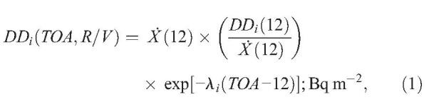
The deposition density DD of a given radionuclide, either deposited on the ground surface or intercepted and retained on vegetation at a particular location, can be estimated from the exposure rate at 12 h post-detonation, X˙(12), and the fallout time-of-arrival, TOA, at the site (as defined by Bouville et al. 2022) using the following equations.

Total deposition density of nuclide i at TOA:

and the deposition density of radionuclide i initially intercepted and retained on vegetation at TOA due to dry deposition is

where

and

A brief description of each of the parameters in eqns (1) through (4) is given below. More detailed discussions of each parameter as well as recommended default values are given in the discussion that follows as well as in the Appendices. Although the model for deposition on vegetation is strictly applicable only for dry deposition because it assumes that the particles deposit via gravitational settling, it can also be applied to wet deposition, although with greater uncertainty, as described later in this paper.

X˙(12) (mR h⁻¹) is the exposure rate at 12 h post-detonation at the location under consideration.

TOA (h) is the fallout time-of-arrival at the location under consideration (as defined by Bouville et al. 2022).

λ_i (h⁻¹) is the radioactive decay constant for nuclide i.

β (Bq m⁻²) is the total beta-particle activity of the fallout deposited at a given location per unit area of ground surface. The model uses beta activity as opposed to total activity¹² because, as discussed in Appendix B, the relationship was developed by regression fits to measured beta activity in soil samples.

DD_i(12)/X˙(12) (Bq m⁻²/mR h⁻¹) is the normalized deposition density of nuclide i at H + 12. DD_i(12)/X˙(12) depends on R/V.

β(12)/X˙(12) (Bq m⁻²/(mR h⁻¹) is the ratio of the total beta activity deposited per unit area of ground (i.e. activity on soil + vegetation) at H + 12 to the exposure rate at H + 12; β(12)/X˙(12) depends on R/V.

(DD_i(12)/β(12))_{R/V = 0.5} is the activity fraction of nuclide i to the total beta activity intercepted and retained by the vegetation evaluated at the reference time t = H + 12 for R/V = 0.5. [DD_i(12)/β(12)]_{R/V = 0.5} is for R/V = 0.5 because only particles <50 μm in diameter are assumed to be intercepted and retained by vegetation and R/V for these particles is assumed to be R/V = 0.5 as discussed later.

N₅₀ is the fraction of the total beta activity that is on less than 50 μm particles deposited per unit area of ground (soil + vegetation) at the location under consideration.

N₀ = N_50-axis is the fraction of the total beta activity that is on less than 50 μm particles deposited per unit area of ground (soil + vegetation) on the trace axis at the same TOA as at the location under consideration.

d is a unit-less parameter that reflects the spread in the width of the fallout pattern with distance downwind due to wind shear.

(1-a) is a unit-less parameter that depends on the height of the burst (HOB) above the ground (Appendix B).

X˙ (mR h⁻¹) is the exposure rate at the location under consideration.

X˙_max (mR h⁻¹) is the exposure rate on the trace axis at the same TOA as at the location under consideration.

t_r (unit-less) = TOA/t_max where t_max (h) is the estimated time for all particles >50 μm to be deposited.

t_max (h) = CT/w_g is the maximum time for all particles >50 μm to deposit due to gravitation, where CT is the height of the stabilized debris cloud (km) and w_g is the gravitational settling velocity of 50-μm particles in km h⁻¹. At times greater than t_max, all particles depositing will be less than 50 μm. Values of t_max for various NTS tests with different fission yields and CT varied from 12 to 16 h for tests with yields ranging from 7 to 44 kt (Table B1, Appendix B).

Table B1.

Characteristics of U.S. and USSR Tests with post-detonation data that was used to estimate values for d and (1-a) and to estimate R/V vs. N₅₀. HOB = height of burst, CT = cloud top altitude above mean sea level (Hawthorne 1979; Gordeev 2000b).

Test	Date	Location	Yield (kt)	Fissile Material	Npb 12/48h	HOB,m	CT(km)
Trinity	7/16/45	Alamogordo	21	a	6/18	30	10.7
Nancy	3/24/53	NTS	24	a	4/13	92	12.6
Badger	4/18/53	NTS	23	a	6.18	92	10.9
Simon	4/25/53	NTS	43	235U	3/10	92	13.4
Tesla	3/1/55	NTS	7	239Pu	3/10	92	9.1
Apple	3/29/55	NTS	14	a	1/4	152	9.8
Met	4/15/55	NTS	22	235U	1/5	122	12.2
Apple2	5/5/55	NTS	29	235U	1/4	152	13.1
Boltzmann	5/28/57	NTS	12	a	<1	152	10.1
Priscilla	6/24/57	NTS	37	235U	1/4	213d	13.1
Diablo	7/15/57	NTS	17	a	3/10	152	9.6
Shasta	8/18/57	NTS	17	a	3/10	152	9.8
Smoky	8/31/57	NTS	44	235U	1/ 5	213	11.6
N2	9/24/51	SNTSc	38	239Pu	X–	30	11.6
N148	8/7/62	SNTS	10	239Pu-	X–	0	5.7
N242	10/14/65	SNTS	1.1	239Pu-	X–	-48	. 55

^a239Pu but significant fraction of fission from uranium (Beck et al. 2020).

^bPercentage of X˙ due to Np at H+12h, H+48h (R/V = 0.5).

^cSNTS (Semipalatinsk nuclear test site, Kazakhstan).

^dBalloon shot.

f_dry is a unit-less parameter that describes the fraction of the deposition density initially retained on the vegetation for a specific radionuclide and vegetation type as a function of particle size Thiessen et al. (2022).

Equations (1) and (2) give estimates of the total deposition density and the deposition density of radionuclide i deposited on and initially retained by vegetation, respectively, as if all the activity had deposited at one time TOA.¹³ In order to estimate the activity of a particular nuclide at TOA, one must correct for radioactive decay as well as any ingrowth from precursors from TOA to 12 h, because the calculated values of DD_i in eqns (1) and (2) are for H + 12. The exponential term in eqns (1) and (2), e^−[-λ_i ^{× (TOA-12)]}, assumes no ingrowth from precursors, which is the case for most of the radionuclides of concern for internal dose (Anspaugh et al. 2022). However, a few important radionuclides are decay products of other nuclides that may not yet have fully grown in at H + 12; thus, eqns (1) and (2) will overestimate the activity at earlier times or underestimate the activity at times > 12 h. An important example is ¹³¹I that grows in from the decay of ¹³¹Te and ^131mTe. The relative deposition density for those nuclides whose activity may not yet have fully grown in at H + 12 is shown in Table 1 for a typical Pu-fueled NTS test, Tesla (Hicks 1981). Note that even at H + 12, only ~90% of the ¹³¹I that will arise from the decay of tellurium precursors has grown in. For these radionuclides, the exponential decay rate term in eqns (1) and (2) needs to be substituted for by the effective in-growth and decay rate correction factors given in Table 1.

Table 1.

Effective in-growth and decay correction factors for radionuclides that contribute significantly to internal dose whose activity vs. time is influenced by ingrowth from precursors. The values in this table are intended to replace the decay term in eqns (1) and (2). The relative activities of ¹³¹Te and ^131mTe are included only to indicate the relative potential ingrowth of ¹³¹I as a function of time. All values are normalized to 1.0 at H=12 h.

TOA	1 h	2 hv	3 h	4 h	6 h	9 h	12 h	18 h	24 h	48 h
91Sr	2.20	2.04	1.90	1.77	1.53	1.24	1.0	0.81	0.42	0.08
91Y	0.08	0.17	0.28	0.38	0.57	0.81	1.0	1.16	1.46	1.74
92Y	1.01	1.59	1.89	1.90	1.91	1.47	1.0	0.40	0.14	0.002
97Nb	0.73	1.03	1.18	1.24	1.23	1.07	1.0	0.88	0.57	0.22
99mTc	0.16	0.29	0.41	0.52	0.69	0.86	1.0	1.07	1.13	0.95
103mRh	0.52	0.77	0.93	0.96	0.99	1.0	1.0	1.0	0.99	0.98
105Rh	0.19	0.36	0.49	0.61	0.78	0.93	1.0	1.01	0.95	0.62
131Te	1130	367	96	23	2.18	1.08	1.0	0.94	0.73	0.41
131mTe	1.07	1.22	1.23	1.20	1.15	1.07	1.0	0.93	0.72	0.41
131I	0.61	0.90	0.98	1.0	1.01	1.01	1.0	1.0	0.95	0.90
133I	1.21	1.30	1.30	1.27	1.22	1.10	1.0	0.90	0.62	0.28
140La	0.093	0.18	0.27	0.36	0.53	0.78	1.0	1.22	1.79	2.88
143Pr	0.066	0.16	0.25	0.35	0.52	0.77	1.0	1.0	1.0	1.0

Equations (3) and (4) estimate the fraction of the total fallout beta activity on particles less than 50 μm, at TOA as a function of t_r = TOA/t_max. Equation 2 requires an estimate of the total beta activity rather than the total radioactivity because, as discussed in Appendix B, the model is based on regression fits to post-detonation measurements of the fraction of total beta activity on particles <50 μm in diameter. Recommendations on how best to use the activity of nuclide i deposited and initially retained on vegetation (eqn 2) to estimate the potential internal exposure and dose for a particular radionuclide deposited on vegetation is discussed in the papers by Thiessen et al. (2022) and Anspaugh et al. (2022). As seen in Fig. 1, the measured values of N_o = N_50-axis for NTS tests follow the model fairly well; i.e., N₀ is very low along the axis of the trace at early times, increasing rapidly as t_r = t/TOA ≤ 1. N₀, however, varies significantly from test to test depending on the values for d and (1 − a), requiring unique estimates of d and (1 − a) for each test. As indicated by eqn (3), N₅₀ also varies with distance from the trace axis according to the relative change in exposure rate for a given TOA; i.e., X˙/X˙_max.

Fig. 1.

Measured vs. calculated N₀ vs. t_r = TOA/t_max for NTS tests [d = 1.8, (1-a) = 0.9].

As indicated earlier, particles larger than about 50 μm in diameter have been shown to generally not be intercepted and retained effectively initially on vegetation. Thus, as discussed in the next section, fallout particles deposited and initially retained on vegetation will be enhanced in volatile nuclides compared to the fallout particles deposited on the ground. Since most of this volatile nuclide activity will be on the surface of these small particles, it will likely be more soluble; i.e., more biologically available (Gordeev 1999). This has significant implications, in particular, for estimating the amount of ¹³¹I on vegetation consumed by cows and on estimating thyroid doses from deposited ¹³¹I (Anspaugh et al. 2022). Equation (2) allows estimates of the fraction of deposited activity capable of being retained on vegetation. However, in some instances, it is also of interest to estimate the fraction of nuclide i activity deposited on the surface soil in order to estimate the intake by animals that ingest significant amounts of soil during grazing, particularly in sparsely vegetated areas. Appendix D provides a method for making such estimates.

Dependence on fractionation

Our model for estimating deposition of radioactive fallout differs from other models of the same purpose in that it accounts for radionuclide fractionation. Previous models often ignored fractionation, particularly at close-in distances,¹⁴ and thus typically overestimated the amount of volatile activity deposited both on the ground and on vegetation close to a test site. Similarly, the increased relative activity of volatile radionuclides on vegetation relative to refractory nuclides at further distances was typically underestimated by assuming a fission product distribution in the fallout based solely on calculated fission yields for either ²³⁵U or ²³⁹Pu.

The basic physics of a nuclear explosion and the resulting effect on the distribution of radionuclides in fallout is discussed in more detail in Appendix A. The fission of the nuclear fuel (fissile material) results in the creation of a large number of fission products and activation products as well as a considerable amount of unfissioned fuel. As illustrated in Fig. 2, as the debris cloud from the fission cools, the various components of the device and products of the fission and activation condense at different temperatures and form liquid oxides.

Fig. 2.

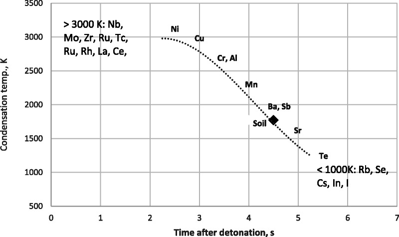
Condensation temperatures of various elements relative to melting temperature of soil as a function of time after detonation for a ~10 kt event (Based on Miller 1963). The time scale varies with fission yield, so for a yield of 20 kt, the time at which soil solidifies would be ~6 s and ~ 9 s for an 84 kt event (Appendix A).

Hicks (1982) inferred from NTS test data that as one moved away from the detonation site, R/V would decrease and asymptotically approach ~0.5. Thus, the distance corresponding to t_max can be taken as the distance corresponding to the distances where Hicks observed R/V to asymptotically approach 0.5 (> a few hundred kilometers for NTS tests with fission explosive yields of ~20–50 kt). Assuming all particles <50 μm have an R/V of 0.5 is thus consistent with Hicks’ findings. Because all the heavy particles are assumed to have deposited by t_max, only small particles (≤50 μm) remain in the cloud. There will continue to be further depletion of larger particles and, thus, some small additional decrease in R/V at further distances. However, subsequent deposition would tend to be governed more by rain-out than gravitation because the rate of gravitational settling for particles < 50 μm is low.

The distribution of the relative nuclide activity vs. time after detonation for near surface NTS tests was calculated by Hicks (1981) for R/V = 0.5 using an appropriately modified version of the ORIGEN computer code (RSIC 1979). The ORIGIN unfractionated activity distributions were then modified to reflect that the relative activities change as the fallout particles separate themselves as a function of distance from the hypocenter due to differences in condensation temperatures of various isotopes and selective deposition by particle size. We extended Hicks’ calculations to provide estimates of the relative nuclide activities for R/V ranging from 0.5 to 5 for a number of these tests.¹⁵ Specified R/V values are actually an average value, and the ratio of activity for a particular refractory nuclide to a particular volatile nuclide may vary slightly from the average because, as discussed in more detail in Appendix A, all volatile elements do not condense at the same time. Thus, the sizes of the debris particles on which the volatile nuclides condense will be smaller for some nuclides such as ¹³⁷Cs, which has a fairly long-lived gaseous precursor and thus an effective condensation time of several minutes compared to the average volatile radionuclide (Fig. 2).

Hicks’ calculations from both NTS and high-yield thermonuclear detonations (Hicks 1981, 1982, 1984) suggest that differences in neutron spectra (due to differences in fissile material) from device to device, while resulting in some differences in the initial nuclide distribution (Appendix A), do not affect the overall average R/V significantly.

Implementation of model

The paragraphs that follow describe in detail how to implement the model to calculate DD_i at a location of interest. It is recommended that the implementation be carried out in the following steps. Each of these steps is discussed in more detail in the following text.

1. Estimate X˙(12) at the location of interest from measured or interpolated values.

2. Estimate TOA at the location of interest from measured or interpolated values.

3. Estimate d from the width of the observed fallout pattern (or use default).

4. Estimate (1 − a) from the HOB (or use default).

5. Estimate the CT and w_g (or use defaults).

6. Calculate t_{max =} CT/w_g; t_r at site.

7. Estimate X˙/X˙_max.

8. Calculate N₅₀ using eqns (3) and (4).

9. Estimate R/V from N₅₀.

10. Estimate DD_i/X˙(12) from R/V using default values based on Hicks.

11. Calculate DD_i-veg at TOA for each nuclide of interest from X˙(12), TOA, the estimated R/V and an appropriate estimate of f_dry from Anspaugh et al. (2022) and Thiessen et al. (2022).

A detailed example of the calculation of DD_{i and} DD_i,veg following the steps above is given in Appendix E.

Some of the parameters in eqns (1) through (4) are event-dependent; i.e., they vary with the fission yield, fuel (fissile material), HOB, etc. Proposed default values based on data from NTS and SNTS nuclear tests are provided in Table 2 that will allow reasonable preliminary estimates of each DD_i, and DD_i,veg. As additional information is obtained on the HOB, CT, explosive yield, etc., one can modify these initial defaults based on the discussions of the variability in each parameter in Appendix C. It is possible that some parameters, such as the yield and/or cloud top height, will not be available immediately, and thus, the initial estimates of N₅₀ and R/V may be very uncertain. However, assuming N₅₀= 1 and R/V = 0.5 at all sites will provide an upper bound estimate of the deposition density of radionuclide i on particles < 50 μm initially intercepted and retained on vegetation at TOA, DD_i /X˙(12) for all volatile radionuclides at close-in distances will be overestimated (and refractory nuclide activities underestimated). However, the activity of volatile nuclides most likely to contribute to the highest internal radiation exposure (radioiodines) will be overestimated. Thus, initial internal dose estimates of volatile nuclides based on this upper bound deposition-density on vegetation will be conservative and likely not underestimate the population dose, while the dose to organs of the gastrointestinal tract from certain refractory nuclides may be underestimated.

Table 2.

Proposed default parameter values for eqns (1) through (4).

Parameter	Default (Y known)a	Default (Y unknown)	Comments
1-a	1X– [0.1 × e-(HOB/70)]	1X– [0.1 × e-(HOB/70)]	0.95 if HOB unknown (HOB; 70 in m)
d	1.6	1.6
CT	1.85 × ln(Y) + 4.7 km	10 km
wg	0.75 to 0.8 km hX–1	0.75 to 0.8 km hX–1	Adjust for latitude—see Appendix C
R/V	0.5	0.5
β(12)/X˙(12)	See text
(DDi(12)/β(12))R/V = 0.5DDi(12)/X˙(12)	See text

^aY is the explosive yield in kt.

Implementation of model: Determining X˙(12), X˙_max from post-detonation monitoring data

The model described here starts with post-detonation exposure rate data. The model assumes that the measurements are of the exposure rate from gamma radiation above an extended soil surface and are representative of the surrounding area. Unfortunately, there will always be limitations in these data. First, the data will be taken at different times and must be decay corrected to our standard reference time, H + 12. Second, the measurements will probably be obtained using different types of instruments and may have to be corrected for varying response as a function of energy. Unless extensive airborne survey data are available, the data will usually be limited to easily accessible areas (e.g., near roads) and interpolation to unmonitored locations may be required.

In this discussion, we will assume that corrections and interpolations can be carried out to delimit the fallout pattern adequately for the purposes of implementing our model. We will, therefore, concentrate on the problem of converting measured or interpolated exposure rates to those at H + 12 and also to estimating TOA at locations of interest. Fortunately, as illustrated in Appendix C, the decay rate is relatively independent of fractionation and fissile material from TOA of ~2 h to several weeks, the time period when most measurements will take place. However, the decay rate will vary from event to event due to other causes such as the amount of activity from activation products, in particular, due to the fraction of activity from ²³⁹Np, which is formed by activation of ²³⁸U. As discussed in Appendix C, all NTS test fallout, even Pu-fueled tests, deposited some ²³⁹Np. For Pu-fueled tests this was due mostly to activation of ²³⁸U in the natural or enriched U used as a tamper but there were possibly also some small amounts of ²³⁸U and ²³⁹Np mixed in with the Pu core material since the ²³⁹Pu was produced from ²³⁸U activation in a reactor. However, ²³⁹Np accounts for a relatively small fraction of the exposure rate during the first few days after the detonation (Appendix C) and thus should not significantly affect the conversion of the measured exposure rate to H12.

As discussed in Appendix C, the change in exposure rate with time also depends on how much weathering takes place with the effect of weathering being minor for the first week or so after the detonation when most survey data would presumably be obtained (Bouville et al. 2022). This assumes significant rainfall does not occur during or immediately after the detonation. In that event, corrections would need to be made to the estimates of X˙(12) from measured X˙ to account for the reduction in exposure rate.

The exposure rate X˙(t) resulting from deposited fallout at each location of interest will vary slightly with the degree of fractionation. However, as shown in Fig. 3, the dependence on fractionation is small (<20%) except for times greater than H + 1,000 h. Thus, not correcting the decay rate for R/V may result in minor errors in estimating cumulative population exposures (Bouville et al. 2022) but will have little effect on correcting monitoring data to H + 12. Hicks’s calculations for NTS tests show that the variation with R/V is also fairly test-independent, i.e., relatively independent of yield and fissile material. The decay rate for a given R/V varies by < 10% from test to test for all times up to a few months post-detonation (Hicks 1981). Examples of decay rates for various NTS tests as calculated by Hicks are given in Appendix C.

Fig. 3.

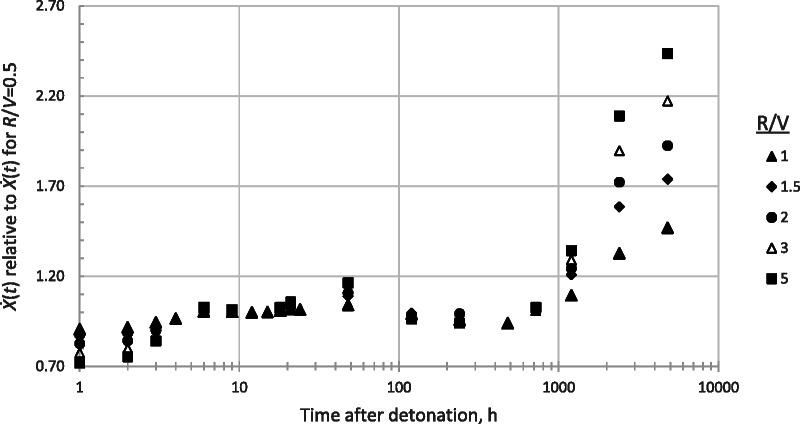
Example of dependence of X˙(t) on R/V, normalized to R/V = 0.5.

Finally, as discussed in Appendix C, the change in exposure rate with time as calculated by Hicks does not reflect the possible small errors due to the dependence of relative volatility for nuclides such as ¹⁴⁰Ba and ¹⁰³Ru on yield and fissile material. However, the possible error is minor over the first few days after a detonation since the exposure rate at these times is due to a large number of short-lived radionuclides, and the few nuclides whose volatility varies with yield account for only a small fraction of the total exposure rate. Furthermore, some of the errors are in opposite directions and thus tend to cancel out.

As shown in Appendix C (Tables C1 and C2), much of the small variation from test to test as calculated by Hicks was due to the fraction of the exposure rate from activation products as opposed to fission products, in particular, the contribution from ²³⁹Np.

Implementation of model: default decay rate (mR h⁻¹)

Many previous investigators have used a t^−1.2 approximation to represent the decay rate. As shown in Bouville et al. (2022), this can result in a significant error in calculating X˙(12) from measurements made either much earlier than 12 h post-detonation or much later. Although as noted above, the exposure rate will vary slightly with yield and degree of fractionation, we recommend a default decay rate representative of a typical NTS test that will provide reasonable estimates of X˙ for all times and be sufficiently accurate for decay-correcting measured X˙(t) to H + 12. For convenience in calculating decay corrections, Hicks exposure rates as a function of H + t, normalized to 1.0 mR h⁻¹ at H + 12 h, calculated for Tesla (Hicks 1981) for R/V = 0.5, were fit to a 10-term exponential (eqn 5) by Henderson (1991). The values of A_i and L_i are shown in Table 3; t in eqn (5) has units of hours:

Table 3.

Values of the fitted regression parameters for eqn (5) (Henderson 1991).

A i	L i
1.033 × 102	X–1.838 × 100
3.206 × 101	X–6.369 × 10X–1
2.476 × 100	X–1.189 × 10X–1
3.476 × 10X–1	X–3.075 × 10X–2
1.332 × 10X–1	X–8.284 × 10X–3
2.851 × 10X–2	X–2.208 × 10X–3
3.302 × 10X–3	X–4.653 × 10X–4
9.055 × 10X–5	X–8.166 × 10X–5
3.692 × 10X–6	X–2.312 × 10X–5
1.003 × 10X–5	X–2.649 × 10X–6

The fit reproduces Hicks’s calculated values to better than 1% at almost all TOA with an overall correlation > 0.99.

Implementation of model: TOA (h)

Besides requiring estimates of X˙(12) at each site of interest, the model also requires an estimate of TOA, the fallout time-of-arrival at the site, as defined by Bouville et al. (2022). To estimate TOA, we recommend the use of either direct or interpolated measurements. If this is not feasible, TOA can be crudely estimated from the downwind distance and an average wind speed. Estimating TOA from ground-level wind speed can be very inaccurate, particularly since cloud-level wind speeds generally are considerably higher than ground-level wind speeds, and there may be significant wind shear that results in fallout occurring along a line and at a distance very different from the direction and speed of the ground-level winds. Estimating TOA from ground-level wind speed will likely overestimate the TOA and result in an overestimate of t_r and N₅₀. Using average wind velocity over the altitudes of the debris cloud, if known, may provide a slightly better estimate¹⁶ (Appendix C). Although a detailed meteorological analysis has been shown to be capable of providing good estimates of TOA for TOA of a few hours or less given detailed metrological data at the detonation site (Bouville et al. 2022), estimates at sites further downwind will be more uncertain, particularly if detailed wind velocity and direction data vs distance and altitude are not available and the distribution of particle activity-sizes in the debris cloud is not known. The uncertainty that can arise from a poor estimate of TOA at a site is discussed in more detail in Appendix C.

Implementation of model: d

Although d can be roughly estimated from measurement of the width of the fallout pattern (Appendix C), unless the fallout pattern is well defined and relatively narrow, it is difficult to do.

As a default we propose d = 1.6, the value recommended for use in the original Russian model (Appendix B)

Implementation of model: (1-a)

As shown in Appendix C, N₅₀ becomes less dependent on (1 − a) as t_r increases. The dependence is really only severe at very close distances (very early TOA) and near the trace axis.

As a default, we propose using the best fit to Fig. B1: (1 − a) = 1 − [0.1 × e^−(z/70)], where z is the height of burst (HOB) in m.

Implementation of model: CT

The height of the stabilized cloud, CT, in km, will depend on the explosive yield (kt) but can vary significantly for the same yield due to local meteorological conditions. Proposed default values are given in Table 2 based on the observed CT data for NTS tests (Appendix C).

Implementation of model: w_g

Gordeev (1999) estimated 0.73 km h⁻¹ as the average gravitational fall velocity, w_g, of 50−μm-diameter spherical particles, density = 2.5 g cm⁻³, at the SNTS. Miller (1963) suggested 0.81X–0.82 km h⁻¹ for NTS detonations for 2.5 g cm⁻³ 50 μm particles. Both are estimates in that the particles are not all perfectly spherical, and the fall velocity varies with the particle density, air viscosity, etc. As a default value, we propose w_{g =} 0.75 to 0.8 km h⁻¹ with the exact choice based on the latitude at which the detonation occurred (Appendix C). Recommended values are 0.75 km h⁻¹ for sites in the latitudes of the continental US south of 35^o latitude and 0.8 km h⁻¹ for sites to the north. The ratio of CT/w_g determines t_max, the critical parameter in determining N₅₀. Appendix C discusses the error in N₅₀ for a given TOA due to an error in estimating t_max.

Implementation of model: N₅₀

As indicated by eqn (3), N₅₀ depends not only on t_r = TOA/t_max but also on the location of the deposition site relative to the axis of the fallout pattern. This is reflected by the ratio of exposure rate off-axis relative to on-axis. As discussed in Appendix B, for the same TOA, N₅₀ increases with distance from the trace axis as the fallout deposition pattern widens as a result of wind shear.

Implementation of model: R/V

In order to apply eqns (1) and (2), one needs to estimate R/V for the fallout at the site of deposition. R/V can be estimated from the calculated value of N₅₀ for a site given an estimate of the relationship between N₅₀ and R/V. As illustrated in Appendix E, R/V can also be estimated from measured ratios of a particular volatile nuclide (usually ¹³⁷Cs) to X˙(12) or to a refractory nuclide such as ⁹⁵Zr where the relevant nuclide activity can be estimated from soil-sample analyses. As shown in Fig. 4, the ratio of DD_Cs-137 to X˙(12) varies considerably with R/V. Although the ratio does also vary with fission yield, type of test and fissile material, these differences are minor compared to the dependence on R/V. Thus, using the dependence of DD_Cs-137 /X˙(12) on R/V shown in Fig. 4 and the observed dependence of DD_Cs-137/X˙(12) on N₅₀ from soil analyses at sites downwind from the NTS, one can estimate the dependence of R/V on N₅₀.

Fig. 4.

Ratio of DD_Cs-137/X˙(12) (Bq m⁻²/mR h⁻¹) vs. R/V for a ²³⁹Pu-fueled device (Tesla), a ²³⁵U-fueled device (Smoky), and two tests (Trinity and Diablo) where the fission was due to a combination of ²³⁵U, ²³⁸U, and ²³⁹Pu (Appendix B, Table B1).

The estimated relationship between N₅₀ and R/V and the measurements of ¹³⁷Cs in soil and corresponding X˙(12) at a number of sites downwind from the NTS and Semipalatinsk test sites used to determine the relationship are discussed in more detail in Appendix C. As discussed in Appendix C, because of the significant uncertainty in the estimated relationship between N₅₀ and R/V, we recommend using the bin grouping shown in Table 4 as a default for R/V as opposed to attempting to estimate more precise values.

Table 4.

Default values for R/V as a function of N₅₀.

N 50	R/V
>0.83	0.5
0.43 to < 0.83	1.0
0.23 to < 0.43	1.5
0.09 to < 0.23	2.0
<0.09	3.0

The use of these binned values will usually provide sufficiently accurate estimates of R/V for use in eqns (1) and (2).

Implementation of model: β(12)/X˙(12)

As shown in Appendix C, β(12)/X˙(12) varies not only with R/V but also with fissile material (i.e., ²³⁹Pu, ²³⁵U, ²³⁸U, etc.) and in particular with the fraction of the beta activity from activation products such as ²³⁹Np. As a default value, we propose (Table 5) the values calculated for NTS test Tesla, a typical Pu-fueled low yield fission device (Table B1, Appendix B) for applying eqn (1) or (2) to a test with unknown fuel and activation product activity.

Table 5.

Default values for β(12)/X˙(12); Bq m^X–2 per mR h^X–1.

R/V	β(12)/X˙(12)
0.5	3.64 × 106
1.0	4.19 × 106
1.5	4.58 × 106
2.0	4.86 × 106
3.0	5.24 × 106

Implementation of model: [DD_i(12)/β(12)]_{R/V = 0.5}; DD_i(12)/X˙(12)

As discussed in the previous paragraphs and the appendices, most of the information required to apply eqns (1) through (4), other than the exposure rate measurements, can be adequately approximated based on Hicks’ calculations (as modified) and regression fits of the model to NTS and SNTS fallout data.

Values for DD(12)/β(12); DD(12)/X˙(12) as a function of R/V for Tesla for each of the radionuclides deemed to account for most of the internal dose (Simon et al. 2022; Anspaugh et al. 2022) are included in Table 6, along with a few additional nuclides that are referred to in the text of this paper and its Appendices. Based on the Hicks calculations for a variety of both Pu and U-fueled devices of different yields (Appendix C), these estimates can be used as default values to estimate Pu for most low yield (~ 5X–25 kt) fission detonations. Again, these are based on Hicks’s calculated relative activities as modified for R/V. For a Pu-fueled detonation, unfissioned plutonium will also be deposited. However, Hicks does not give values for Pu since the unfissioned plutonium from Tesla (and all other NTS tests) is still classified. The actual Pu deposition for any Pu-fueled detonation will depend on the amount of Pu in the device and the efficiency of fission. In Table 6, we have assumed default ^239+240Pu to X˙(12) activity ratios based on data for the Trinity test (Beck et al. 2020). These Pu-deposition density values are intended to provide a crude order-of-magnitude initial estimate that could possibly be revised at a later date when additional information becomes available. The actual deposition density of ^239+240Pu will depend on the construction of the device and could vary considerably from these estimates (a factor of two or more for a low efficiency detonation). The initial estimates of Pu-deposition density will need to be validated based on subsequent measurements of fallout-contaminated soil at the location of interest or of the debris cloud.

Table 6.

Default values for DD_i/β; DD_i/X˙ at H+12 h derived for Tesla (Pu from Trinity-see text).

		DDi/β at H+12 h	--------------DDi/X˙ at H+12 h; Bq mX–2/mR hX–1 ----------------
Nuclide	T1/2	R/V = 0.5	R/V = 0.5	1	1.5	2	3	5
89Sr	50.6 d	8.39 × 10X–4	3.04 × 10+3	2.48 ×10+3	2.09 ×10+3	1.81 ×10+3	1.43 ×10+3	9.99 ×10+2
90Sr	28.9 a	4.52 × 10X–6	1.64 × 10+1	1.34 ×10+1	1.13 ×10+1	9.79 ×10+0	7.73 ×10+0	5.40 ×100
90Y	64.1 h	4.52 × 10X–6	1.64 × 10+1	1.34 ×10+1	1.13 ×10+1	9.79 ×10+0	7.73 ×10+0	5.40 ×100
91Sra	9.65 h	4.84 × 10X–2	1.75 × 10+5	1.69 ×10+5	1.60 ×10+5	1.54 ×10+5	1.45 ×10+3	1.36 ×10+5
91Ya	58.5 d	4.29 × 10X–4	1.55 × 10+3	1.50 ×10+3	1.42 ×10+3	1.37 ×10+3	1.29 ×10+3	1.21 ×10+3
92Sr	2.66 h	1.21 × 10X–2	4.37 × 10+4	7.14 ×10+4	9.03 ×10+4	1.04 ×10+5	1.23 ×10+5	1.44 ×10+5
92Y	3.54 h	4.16 × 10X–2	1.51 × 10+5	2.46 ×10+5	3.11 ×10+5	3.59 ×10+5	4.24 ×10+5	4.95 ×10+5
93Y	10.2 h	3.95 × 10X–2	1.35 × 10+5	2.33 ×10+5	2.95 ×10+5	3.41 ×10+5	4.02 ×10+5	4.70 ×10+5
95Zr	64 d	7.26 × 10X–4	2.63 × 10+3	4.29 ×10+3	5.43 ×10+3	6.26 ×10+3	7.40 ×10+3	8.64 ×10+3
97Zr	16.7 h	4.09 × 10X–2	1.48 × 10+5	2.42 ×10+5	3.06 ×10+5	3.53 ×10+5	4.17 ×10+5	4.87 ×10+5
97Nb	72.1 m	4.40 × 10X–2	1.59 × 10+5	2.60 ×10+5	3.29 ×10+5	3.79 ×10+5	4.48 ×10+5	5.23 ×10+5
99Mo	66 h	1.85 × 10X–2	6.70 × 10+4	1.09 ×10+5	1.38 ×10+5	1.60 ×10+5	1.89 ×10+5	2.20 ×10+5
99mTc	6.0 h	1.27 × 10X–2	4.59 × 10+4	7.50 × 10+4	9.49 × 10+4	1.09 × 10+5	1.29 × 10+5	1.51 × 10+5
103Rua	39.2 d	3.20 × 10X–3	1.16 × 10+4	9.45 ×10+3	8.01 ×10+3	6.92 ×10+3	5.45 ×10+3	3.81 × 10+3
103mRha	56.1 m	3.20 × 10X–3	1.16 × 10+4	9.45 ×10+3	8.01 ×10+3	6.92 ×10+3	5.45 ×10+3	3.81 × 10+3
105Ru	4.4 h	8.19 × 10X–2	2.96 × 10+5	2.42 ×10+5	2.04 ×10+5	1.77 ×10+5	1.39 ×10+5	9.71 ×10+4
105Rh	35.4 h	4.82 × 10X–2	1.74 × 10+5	1.42 ×10+5	1.20 ×10+5	1.04 ×10+5	8.18 ×10+4	5.73 ×10+4
106Ru	372 d	4.74 × 10X–4	1.72 × 10+3	1.40 ×10+3	1.18 ×10+3	1.02 ×10+3	8.06 ×10+2	5.65 ×10+2
131m Te	30 h	6.06 × 10X–3	2.19 × 10+4	1.79 ×10+4	1.51 ×10+4	1.31 ×10+4	1.03 ×10+4	7.22 ×10+3
131I	8.03 d	9.48 × 10X–3	3.43 × 10+4	2.80 ×10+4	2.36 ×10+4	2.04 ×10+4	1.61 ×10+4	1.13 ×10+4
132Te	3.2 d	2.53 × 10X–2	9.14 × 10+4	7.47 ×10+4	6.30 ×10+4	5.45 ×10+4	4.29 ×10+4	3.01 ×10+4
132I	2.3 h	2.60 × 10X–2	9.40 × 10+4	7.68 ×10+4	6.48 ×10+4	5.60 ×10+4	4.41 ×10+4	3.09 ×10+4
133I	20.8 h	1.04× 10X–1	3.77 × 10+5	3.08 ×10+5	2.60 ×10+5	2.25 ×10+5	1.77 ×10+5	1.24 ×10+5
135I	6.6 h	1.11 × 10X–1	4.03 × 10+5	3.29 ×10+5	2.80 ×10+5	2.40 ×10+5	1.89 ×10+5	1.33 ×10+5
137Cs	30.1 a	1.09 × 10X–5	4.75 × 10+1	3.23 ×10+1	2.73 ×10+1	2.36 ×10+1	1.86 ×10+1	1.30 ×10+1
140Baa	12.8 d	6.35 × 10X–3	2.30 × 10+4	2.22 ×10+4	2.15 ×10+4	2.10 ×10+4	2.04 ×10+4	1.96 ×10+4
140Laa	1.68 d	1.20 × 10X–3	4.33 × 10+3	4.17 ×10+3	4.05 ×10+3	3.96 ×10+3	3.84 ×10+3	3.70 ×10+3
141Laa	3.92 h	4.91 × 10X–2	1.78 × 10+5	2.18 ×10+5	2.45 ×10+5	2.65 ×10+5	2.93 ×10+5	3.22 ×10+5
142La	1.59 h	3.71 × 10X–3	1.34 × 10+4	2.19 ×10+4	2.78 ×10+4	3.20 ×10+4	3.78 ×10+4	4.42 ×10+4
143Ce	1.38 d	2.33 × 10X–2	8.44 × 10+4	1.38 ×10+5	1.74 ×10+5	2.01 ×10+5	2.38 ×10+5	2.77 ×10+5
143Pr	13.6 d	6.42 × 10X–4	2.32 × 10+4	3.80 ×10+4	4.77 ×10+4	5.55 ×10+4	6.55 ×10+4	7.64 ×10+4
144Ce	285 d	1.17 × 10X–4	4.25 × 10+2	6.95 ×10+2	8.80 ×10+2	1.02 ×10+3	1.20 ×10+3	1.40 ×10+3
144Pr	0.29 h	1.17 × 10X–4	4.25 × 10+2	6.95 ×10+2	8.80 ×10+2	1.02 ×10+3	1.20 ×10+3	1.40 ×10+3
145Pr	6.0 h	3.02 × 10X–2	1.09 × 10+5	1.78 ×10+5	2.26 ×10+5	2.60 ×10+5	3.07 ×10+5	3.59 ×10+5
239Np	2.36 d	1.16 × 10X–1	4.18 × 10+5	6.83 ×10+5	8.65 ×10+5	9.97 ×10+5	1.18 ×10+6	1.37 ×10+6
239+240Pu	2.4 × 104 y	X–	1.7	2.7	3.3	3.0	4.3	X–
(β(12)/X˙(12)	X–	X–	3.64 × 10+6	4.21×10+6	4.59 ×10+6	4.87 ×10+6	5.25 ×10+6	5.66 ×10+6

^aDepends on yield and fissile material and, thus, the R/V for that nuclide may be slightly greater or less than values estimated by Hicks.

As discussed in Appendix A, the relative volatility of a few of these nuclides (as indicated in Table 6) depends on yield and fissile material, and thus the R/V for that nuclide may be slightly greater or less than values estimated by Hicks.

Dry deposition vs. wet deposition

The estimates of N₅₀ using eqns (3) and (4) assume dry fallout, i.e., particle size is governed by gravitational settling only. Although our model is strictly applicable only for dry deposition, it can also be applied to wet deposition, particularly eqn (1), if one recognizes the increased uncertainty. First, because rain-out and wash-out will likely increase the probability of more of the smaller particles in the air and cloud being deposited at an earlier time, the average R/V at the site will likely be reduced, and the fraction of total activity on < 50 μm particles will likely be greater. However, the fraction of that activity initially intercepted and retained on vegetation may be smaller than for dry fallout (Hoffman et al. 1992; Thiessen et al. 2022). The fallout depositing on some surfaces such as road surfaces, roofs, etc., may be intercepted but immediately be redistributed in a manner that may change the relative nuclide activity. The shift in R/V will only be significant in the areas where R/V would be >> 0.5 for dry fallout, i.e., near the trace axis and near GZ. For most sites, R/V would still be ~0.5. It should be noted that as the particle sizes continue to decrease with increasing distance,¹⁷ gravitational settling becomes insignificant, and rainfall processes account for most of the fallout deposition. This was observed in most studies of long-range tropospheric fallout (NCI 1997; Bouville and Beck 2000). However, wet deposition may change the distribution of nuclides deposited vs. distance. Additional data (e.g., precipitation analyses of the ratio of volatile to refractory nuclides) may be required to accurately model R/V.

UNCERTAINTY

A detailed discussion of the uncertainty in each parameter in eqns (1) through (4) is given in Appendix C. Although some of our uncertainty estimates are fairly crude, most have a relatively minor impact on the estimates of internal dose because the total uncertainty in internal dose involves many other parameters with even greater uncertainty (Anspaugh et al. 2022; Thiessen et al. 2022). A detailed uncertainty analysis was performed in conjunction with the application of this methodology to a reconstruction of thyroid doses at sites downwind from the USSR SNTS (Land et al. 2015). That analysis estimated the uncertainty in each of the major parameters in eqns (1) through (4) and assigned probability distributions to each. These probability distributions were then used to estimate the overall uncertainty in the estimates of internal dose using a 2D Monte Carlo analysis. A sensitivity study based on the uncertainty estimates discussed in Appendix C of this report found that of the parameters in eqns (1) through (4), the one most affecting the uncertainty in the estimate of pasture ¹³¹I activity on vegetation at sites with high fallout, was the uncertainty in N₅₀. The uncertainty in DD_i-veg due to the uncertainty in estimating the average R/V at a site was relatively minor compared to the uncertainty in N₅₀.

The estimate of R/V from N₅₀ is somewhat crude and, as discussed earlier, depends on the specific fissile material in the device. Also, the assumption that only particles <50 μm in diameter are initially retained on vegetation may not hold for all types of vegetation. However, the dependence of X˙(12) on R/V is somewhat independent of the specifics of the detonation, and DD_i(12)/X˙(12) is sensitive to N₅₀ only for a small downwind area near the axis of the fallout trace. Although the estimates of N₅₀ are somewhat uncertain, N₅₀ values only << 1 occur and thus have a significant impact on the estimated nuclide distribution close in and close to the fallout trace axis. In those areas, the fraction of the activity on small particles that are enriched in volatile nuclides, in particular iodines, will be reduced relative to areas farther away or farther from the fallout trace axis. Thus, ignoring fractionation for close-in sites gives conservative estimates for the activity of volatile nuclides such as iodines on vegetation. Away from the fallout trace axis or at distances > t_max, where all the particles are <50 μm, DD_i-veg depends on the assumption that R/V is ~0.5. Neglecting this fractionation for these larger, albeit lower fallout areas can result in significant underestimates of DD_i-veg for volatile nuclides such as ¹³¹I and significant overestimates for refractory nuclides and thus could result in significant errors in the estimated population dose. In most of the area outside of the heavier fallout areas, the uncertainty in N₅₀ is moot, and the uncertainty in DD_i-veg is due mainly to the relatively small uncertainty in Hicks’s estimates of DD_i(12)/β(12) at R/V = 0.5 and the uncertainty in X˙(12).

Although there is some uncertainty in using Hicks’s estimates of DD/β vs. R/V that are strictly valid for relatively high yield tests (Appendix A), we believe that this uncertainty is minor for most of the radionuclides of interest compared to the uncertainty in estimating N₅₀. However, one should be aware of the potential error in estimating DD(12)/X˙(12) for the particular nuclides that depend on yield and fissile material (Table 6 and Appendix A).

SUMMARY AND CONCLUSION

The model described in this paper can be used to rapidly estimate the deposition density of important radionuclides that can result in internal dose to a downwind population from a nuclear detonation that might occur in the future. One can estimate the deposition density of any fallout radionuclide from any nuclear detonation from the measured exposure rate, normalized to H + 12, and the estimated TOA and R/V using eqns (1) through (4) and following the steps suggested in the section on implementation of the model.

There are a few requirements and caveats:

• An estimate of TOA is required either from direct observations (preferred) or based on estimates/measurements of wind speed vs. altitude. If TOA was not based on actual exposure-rate data, any significant wind shear vs. altitude may preclude an accurate estimate of TOA from wind-speed data;

• The value of d will vary depending on test conditions, and for severe wind shear, the model may not provide reliable estimates of deposition density;

• A fairly comprehensive set of exposure-rate measurements is required to estimate off-axis and on-axis X˙(12). However, one can assume post-detonation aerial and ground surveys will be available within a few days to provide a fairly detailed pattern of exposure rate, and current measurement technology allows fairly accurate estimates of not only exposure rate but also selected radionuclide activities in soil. Measured exposure rates need to be decay-corrected to H + 12 so well documented exposure-rate data are required;

• The estimates of DD_i(12)/X˙(12) assume no remediation has taken place at the site. If it is not the case, this might result in a significant underestimate of X˙(12); and

• The deposition-density estimates assume a relatively flat semi-infinite geometry (radius of at least ~15 m). Otherwise, the conversion from deposition density to exposure rate used by Hicks is not strictly valid (NCRP 1999; Bouville et al. 2022). Although application of the model is intended to start with exposure-rate data, data on deposited activity (i.e., total beta, or deposition density of specific radionuclides) can also be used. In some instances, aerial gamma-spectrometric surveys or subsequent soil sampling might be used to measure the deposition density of a particular radionuclide, usually ¹³⁷Cs, to supplement post-explosion exposure-rate surveys for more distant sites where exposure rates have not been monitored or levels are too low to detect easily. Such measurements can and have been carried out many months and even years after a nuclear detonation.

The model allows one to start with an estimate of the ratio of the deposition density of any volatile to any refractory radionuclide and reconstruct X˙(12) for the site after estimating R/V (Appendix E). For example, measurements of ¹³⁷Cs/⁹⁵Zr or ¹³⁷Cs/Pu in soil can allow one to estimate R/V to confirm estimates based on the model estimates of N₅₀ and measured X˙(12). Thus, one can use soil-sample analyses of specific radionuclides taken weeks or months (or even years) later to validate and improve the initial assessments.

In the event that the only available data for some areas are estimates of the deposition density of ¹³⁷Cs, one can still make crude estimates, as illustrated in Appendix E, of X˙(12) and DD_i(12)/X˙(12) provided TOA can be estimated.

For prospective dose estimations, interdiction may limit the intake of the more volatile nuclides deposited on vegetation, and thus the dose from the fallout will be primarily from external exposure and inhalation. In this case, the uncertainty in the deposition-density model will have less impact on the estimates of total dose. However, in assessing (reconstructing) doses retrospectively at the Nevada Test Site, Semipalatinsk Nuclear Test Site, Marshall Islands, and from the Trinity detonation in New Mexico, no interdiction was assumed to have been carried out, implying that the impact of fractionation was significant, particularly for estimated thyroid doses. Thus, documenting the methodology used for those studies was an important goal of this paper and may prove necessary for future retrospective assessments if adequate interdiction is not carried out.

Although the model described herein is primarily intended for dry fallout, it can be used also for wet deposition (rain-out/wash-out), albeit with less accuracy.

As discussed in the Introduction, the proposed methodology is intended mainly for estimating deposition density from detonations near the ground surface that result in significant local fallout; i.e., for distances of a few hundred km from the detonation site where the TOA is generally < 48 h. However, in principle, the methodology can be used out to much greater distances and TOA, limited only by the ability to accurately determine the H + 12 exposure rate and corresponding TOA. However, as the distance (and corresponding TOA) increases, the exposure rate from fallout may need to be inferred from soil sample analyses rather than direct measurements and any significant fallout is more likely to occur due to precipitation rather than gravitational settling, leading to greater uncertainty.

The methodology can also be applied to high altitude detonations with some modification. Because the fireball from higher altitude detonations does not intersect the ground surface, significant fractionation does not occur [i.e., R/V = 1 (Hicks 1982)], and fallout radionuclides are all on particles < ~20 μm (Freiling and Kay 1965). Thus, the deposition density on both the ground surface and on vegetation should be estimated from X˙(12) and TOA using eqn (1) and DD_i(12)/X˙(12) for R/V = 1.0 from Table 6.

The estimated deposition densities using our model are expected to be at least as, if not more, accurate than estimates made using debris cloud and atmospheric transport models, since the latter require very precise meteorological data which will generally not be available to obtain accurate estimates at more than a few hundred kilometers downwind. As noted earlier, this model has been used successfully to reconstruct doses in several retrospective assessments. Hicks’s DD_i(12)/X˙(12) ratios were originally developed for and used in the Offsite Radiation Exposure Review Project (ORERP) to estimate doses downwind from the NTS (Church et al. 1990). The model has recently been shown to provide good agreement between measured and predicted plutonium-deposition density values at various locations downwind from the Trinity detonation site (Beck et al. 2020).

APPENDIX A—FRACTIONATION

Basic physics of a nuclear detonation

A basic fission device uses either ²³⁵U or ²³⁹Pu or a combination as the fissionable fuel. The fission of this fuel results in the creation of a large number and quantity of fission products and activation products as well as a considerable amount of radioactive debris composed of unfissioned fuel.

The distribution of fission products created in the explosion varies with type of fuel as shown in Fig. A1.

Fig. A1.

Fission yields (%) for ²³⁵U, ²³⁸U, and ²³⁹Pu (from England and Ryder, 1994).

The extreme heat of the blast created by the explosion results in all of these fission and activation products as well as the device components and unfissioned fuel being vaporized into a hot gas that rises into the atmosphere until stabilizing at some height (CT) that depends on the yield and height of burst (HOB).

The soil drawn into the fireball will be vaporized and along with fission products distributed non-uniformly with height and radius of the debris cloud (Cederwall and Peterson 1990; Ralph et al. 2014). For a near-surface burst, on average about 80X–90% of the activity is in the main cloud and about 10X–20% in the stem (Ralph et al. 2014).

The amount and sizes of available condensation particles depend on the height of burst and the composition of the device. If the HOB is low enough, the fireball will intercept the ground surface, and a large amount of soil will be entrained into the debris cloud providing a source of condensates. Other available condensates include the components of the device, unfissioned fuel, and ordinary atmospheric aerosols.

Fractionation

Fractionation refers to the processes that cause the activity distribution of nuclides deposited in fallout at various times post-detonation to differ from the original fission-product distribution created in the explosion. Initially, the relative activity of the various radionuclides in the stabilized debris cloud is determined by the fissile material in the device (e.g., ²³⁵U, ²³⁸U, ²³⁹Pu).

As shown in Fig. A1, this initial fission-product distribution has roughly the same shape for all major fissile materials but does vary slightly with fissile material, particularly for atomic masses of ~100X–130. Some NTS tests where the primary fission was due to ²³⁵U or ²³⁹Pu, but where either natural U or depleted uranium was used as a tamper, also had additional yield due to fission of ²³⁸U by the higher energy fission neutrons produced from the fission of ²³⁵U or ²³⁹Pu. In addition, some of the later higher yield NTS tests utilized “boosting” by adding small amounts of tritium to the fuel resulting in the production of additional fission from fusion-produced 14 MeV neutrons. Thus, the actual fission spectrum for NTS tests varied from event to event depending on the fissile material as well as the tamper material. Furthermore, the distribution of radionuclide activity in the debris cloud changes with time due to the decay of the original fission products and ingrowth of decay products. The distribution of activity in the fallout deposited at any time will differ also from the original distribution due to the variation in the amounts of specific radionuclides deposited on or incorporated into particles of various sizes and the rates at which particles of various sizes deposit gravitationally from various levels of the debris cloud.

Initially, because of the extremely high temperatures, all fission and activation products as well as device components and soil swept up into the cloud are all completely vaporized. As the cloud cools, the soil entrained into the cloud and the iron components of the device tend to liquefy first at about 3,000 °C. As the cooling continues, the more refractory fission products will condense first. These refractory nuclides will be incorporated into the volume of the liquid soil drops, which then solidify. As the temperature decreases to below 1,500 °C, nuclides still in gaseous form start to condense. As the cloud continues to cool to ambient temperature, ~50 °C, these volatile elements (except for noble gases such as Kr and Xe) and their progeny condense and deposit on the surface of the solidified soil and device particles. Because the average particle size of the solidified particles remaining in the debris cloud decreases with time due to gravitational settling, the relative amounts of specific volatile nuclides on the surface of particles will vary with time depending on the time (temperature) at which these nuclides condense. Furthermore, because the surface to volume of a particle varies as ~1/r, the relative amounts of volatile vs. refractory nuclides associated with a particle will vary with particle size and thus with time.

At some point in time, depending on the maximum height of the debris cloud and the vertical fall rate of various size particles, all particles greater than a given size (mass) will deposit leaving only particles less than that mass still in the cloud.

In summary, fractionation is two-step process:

1. Due to varying condensation times, refractory nuclides, i.e., those that condense at temperatures above 1,500 °C, tend to be incorporated into the volume of soil particles, while volatile nuclides that condense after the liquefied soil solidifies are deposited on the surface of solidified particles. Because the volume-to-surface ratio of a particle is approximately proportional to its radius, the relative amounts of refractory vs. volatile nuclides associated with a particle will approximately increase proportionally to their size; and

2. As the cloud stabilizes, the heavier particles will fall out first due to gravitation, so early fallout will consist of larger particles enriched in refractory nuclides.

The net effect is that particles that deposit close-in to the detonation site will be heavier on average and enriched in refractory elements, while particles deposited at further distances will have a smaller median mass and be enriched in volatile elements. However, even at close distances from the detonation site, some smaller particles from the lower levels of the debris cloud will still deposit gravitationally and reach the surface at the same time as larger particles from higher regions in the cloud.

Hicks (1981) defined the nuclides still in gaseous form at 1,500 °C as volatile nuclides, while nuclides that had condensed at temperatures above 1,500 °C were designated as refractory elements. As discussed in the main text, the overall degree of fractionation in fallout is generally characterized by the ratio R/V where R refers to the activity fraction of refractory nuclides in the fallout and V is the fraction of volatile nuclides in the fallout relative to that produced by the detonation. Furthermore, Hicks assumed, based on empirical NTS fallout data, that about half the refractory nuclides would deposit close-in, i.e., be on the larger particles. Once all the larger particles had deposited, the remaining particles would contain a refractory-to-volatile activity ratio of about 0.5 relative to the R/V ratio produced in the detonation and would remain at that average relative volatility independent of changes in particle size with time (i.e., distance). This clearly is an approximation since, as discussed in the main text and illustrated by Crocker et al. (1965) and Miller (1963), the smaller particles will be slightly more enriched in ¹³⁷Cs than iodine or ⁹⁰Sr. Furthermore, the particles sizes will continue to decrease with distance and time and thus become even more enriched in volatile nuclides.

Post-detonation monitoring data from NTS and SNTS nuclear tests confirm the expected impact of fractionation on the activity vs. particle size of fallout vs. distance and TOA. Fig. A2, using data from Baurmash et al. (1958), shows the change in activity median diameter (AMD) vs. t_r for NTS detonation Apple.

Fig. A2.

Illustration of variation in activity median diameter (AMD) with t_r. Data from Baurmash et al. (1958) for NTS test Apple.

As can be seen in Fig. A2, the early fallout from weapons tests was characterized by very large particles on average. Also, as shown in Fig. A3, again using data from Baurmash et al. (1958) for NTS test Apple, the fraction of activity on particles < 50 μm increased as the median size of the fallout particle sizes continued to decrease. At distances close to GZ, one would thus expect the fraction of the most volatile elements such as ¹³⁷Cs to be severely depleted in fallout, as was observed for NTS tests (McArthur 1991).

Fig. A3.

Fallout particle size distribution (AMD) vs percentage of activity on particles less than 50 μm. Data from Baurmash et al. (1958) for NTS test Apple.

Since the smaller particles are enriched in volatile nuclides, the average R/V of the fallout decreases with time as the more refractory large particles continue to be removed from the main debris cloud and the average particle size of the fallout decreases. The smaller the particle sizes of the fallout being deposited, the greater the relative fraction of V vs. R, i.e., the lower the ratio of R/V.

Estimates of relative volatility of individual radionuclide fission chains

Hicks (1982) concluded that for all but three fission chains, all the chain members were either refractory or volatile at 20 s after the explosion, the time he estimated the cloud temperature would reach 1,500 °C. The nuclide chains that are all volatile, partly volatile, or all refractory according to Hicks are indicated in Table A1 along with Hicks’s estimate of the fraction of each chain that is refractory¹⁸. The members of each fission chain with significant fission yields are shown in parentheses. For comparison, estimates of relative volatility by Crocker et al. (1965) for a 20 kt-NTS Pu-fueled test (Smallboy 1962) using a semi-empirical model are also provided. A theoretical prediction of relative volatility for an 84 kt Pu-fueled test (Miller 1963) is also shown in Table A1. Note that Hicks (1982) did not distinguish between Pu and U-fueled tests in his estimates of relative volatility.

Table A1.

Relative degree of volatility (% V) of various fission chains. Precursors with significant fission yields are shown in parentheses.

Nuclide chain	Hicks (1981)	Crocker et al. (1965) a	Miller (1963)
89Sr (Br → Kr →> Rb → Sr)	100	100	99
90Sr (Br → Kr → Rb → Sr)	100	73	97
91Y (Br → Kr → Rb →Sr → Y)b	75	51	X–
95Zr-Nb (Rb → Sr → Y → Zr → Nb)	0	0	1
97Zr-Nb (Rb → Sr → Y → Zr → Nb)	0	X–	X–
99Mo (Sr → Y → Zr → Nb → Mo)	0	4	4
103Ru (Zr → Nb → Mo → Tc → Ru)b	100	52	65
105Rh (Nb → Mo → Tc → Ru → Rh)	100	X–	X–
106Ru,Rh (Nb → Mo → Tc → Ru)b	100	89	55
131I (In → Sn → Sb → Te → I)	100	84	92
132I (Sn → Sb → Te → I)	100	90	96
133I (Sn → Sb → Te → I)	100	X–	99
136Cs (Te → I → Xe → Cs)b	100	65	X–
137Cs (Te → I → Xe → Cs)	100	120	99
140Ba,La (I → Xe → Cs → Ba → La)b	70	53	86
141Ce (Xe → Cs → Ba → La → Ce)b	33	43	42
143 Ce-Pr (Xe → Cs → Ba → La → Ce)	0	X–	1
144Ce-Pr (Xe → Cs → Ba → La → Ce)	0	0.03	0
145-149 mass chains	0	X–	X–
239Np (U → Np)	0	46	X–

^aRelative to 100% for ⁸⁹Sr.

^bIndicates partially volatile chains where the degree of volatility depends significantly on explosive yield.

Because most fission products in fallout are a product of the decay of a number of short-lived members of a fission chain where the precursors are each created with different fission yields, the actual degree of volatility of a given nuclide may differ from the volatility of the final member of the chain. For example, some of ¹⁴⁰Ba, which is refractory, is formed by the decay of precursors that are all volatile (Xe, Cs, i.e., still in gaseous form when soil solidifies). Thus, while Ba condenses before the soil solidifies, some of the precursors that eventually decay into ¹⁴⁰Ba will have not yet condensed.

Note that both the Crocker et al. (1965) and Miller (1963) model estimates reflect small variations in volatility between chains considered all volatile by Hicks, e.g., ¹³⁷Cs and ⁹⁰Sr and ¹³¹I. Because some nuclides such as ¹³⁷Cs condense much later than others, the smaller particles are enriched in these specific volatile nuclides even more than on average. Thus, ¹³⁷Cs is slightly more volatile than ⁹⁰Sr or ¹³¹I.

The estimates of relative volatility for some nuclides by Crocker et al. (1965) and Miller (1963) differ from Hicks (1982) for a few other nuclides because the relative volatility of the different members of a fission chain depends on the time to reach 1,500 °C. As discussed below, the time to reach 1,500 °C depends on the yield and for low yields is actually much less than the 20 s assumed by Hicks. Thus, the relative volatility of the three chains cited as partially refractory by Hicks will vary slightly with yield, which accounts for some of the differences between the comparisons shown in Table A1. As suggested by the different estimates in Table A1, a few additional chains (103, 106) may also be slightly less volatile at lower yields than Hicks’s estimates.

Crocker et al. (1965), also claimed that ²³⁹Np, produced by activation of ²³⁸U, was partly volatile based on his analyses of his data from the Smallboy test, as opposed to Hicks, who assumed uranium is refractory. As discussed in Appendix C, fallout from all NTS tests contained some ²³⁹Np, and a few tests that used uranium tampers, particularly Trinity, produced significant amounts of ²³⁹Np. This not only impacted the average R/V but also the exposure rate at times greater than about 24 h. Although there is some question regarding the volatility of ²³⁹U, the precursor to ²³⁹Np, it is doubtful that future events will use the massive U tampers used in early NTS tests. Thus, the uncertainty in Np volatility should not result in significant additional uncertainty in estimating DD_i(12)/X˙(12) for other nuclides or in correcting exposure rates to H + 12.

Miller (1963) developed a model to estimate the relative volatility of various fission products from different yield fission detonations that attempted to account for the complex chemistry taking place in the debris cloud vs. time. Fig. A4 shows the relative volatility of various nuclides as calculated by Miller for an 84-kt test.

Fig. A4.

Calculated relative volatility for an 84 kt fission detonation. Data from Miller 1963.

Freiling (1961, 1962, 1963; Freiling et al. 1965) developed a semi-empirical model of the relative fractionation of particular nuclides vs. time by plotting the logs of observed ratios of each nuclide activity, A_i to the activity of ⁸⁹Sr, i.e.,

where a and c are fit parameters [this a is unrelated to the a in (1-a) discussed above].

Based on data from various NTS and Pacific tests, Freiling et al. (1965) estimated the relative activities of various nuclides (i.e. values of the parameter c in eqn A1). The Freiling model estimates for relative volatility are in relatively good agreement with the Miller model results considering they were not adjusted for yield and are based on data from a variety of tests of different types. Freiling et al. (1965) also estimated the fraction of total activity for a given radionuclide that would be deposited onto or adsorbed into particles <50 μm (Table A2). The third column of Table A2 presents experimental data from a low yield surface detonation and shows (second column) relatively good agreement with the model prediction. The isotope ratios in the model were all normalized to the expected ratio for no fractionation. The Freiling model results are consistent with the assumptions made by Hicks and our model that at large distances where the particle sizes are all <50 μm, the overall R/V will be on the order of 0.5 on average but also indicates that the relative volatility varies for specific volatile nuclide chains.

Table A2.

Estimated and measured values of the fraction of total activity of nuclide on particles of <50 μm (Freiling et al. 1965).

Nuclide	Model	Measured
137Cs, 89Sr	0.9	0.9
90Sr	0.85	0.85
132I	0.74	0.7
140Ba	0.7	–
132Te	0.63	–
95Zr, 99Mo	0.35	0.2

Consistent with the Freiling fractionation model, the relative volatility of even the most volatile nuclides varies slightly according to the time (temperature) at which they condense. This implies that the longer it takes for nuclides to condense, the smaller the available particle sizes are to which they can attach. Thus, the relative volatility of all volatile fission chains (particularly A = 89, 90, 137) will vary slightly and depend on time, since the average particle size decreases with time.

Using the Hicks’ ratio of ¹³⁷Cs/⁹⁰Sr for a Pu-fueled test, and adjusting the ratio of Cs/Sr volatility based on the Freiling model predictions, Fig. A5 shows the estimated dependence of the ratio of ¹³⁷Cs/⁹⁰Sr on R/V (normalized to 1.0 at R/V = 1.0).¹⁹

Fig. A5.

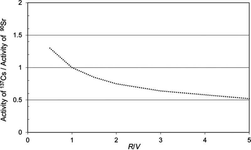
Estimated variation of ¹³⁷Cs/⁹⁰Sr activity vs. average R/V (normalized to 1.0 at R/V = 1.0).

Note that as R/V increases, i.e., at close-in locations at early times, the ratio of ¹³⁷Cs/⁹⁰Sr decreases and at R/V = 0.5 is greater than 1.0. This is due to the effective greater volatility of ¹³⁷Cs that results from both ¹³⁷Cs and ⁹⁰Sr having gaseous precursors. The half-life of ¹³⁷Xe (3.8 min) is much greater than that of ⁹⁰Kr (32 s), and thus the ¹³⁷Cs condenses onto the available slightly smaller cloud particles much later than ⁹⁰Sr. Since, as suggested by Freiling et al. (1965) and Miller (1963), ⁹⁰Sr is slightly more volatile than other volatile chains such as ¹³¹I, the ratio of ¹³⁷Cs/¹³¹I would be expected to be slightly greater than the ratio of ¹³⁷Cs/⁹⁰Sr at R/V = 0.5 relative to R/V = 1.0. Because of the long time for ¹³⁷Cs to condense and attach to particles, the effect would be expected to be increasingly greater as the average fallout particle size decreases.

As discussed, the relative volatilities calculated by Miller (1963), Freiling et al. (1965), and Crocker et al. (1965) are in qualitative agreement with Hicks’s model. However, as discussed above, there are some clear differences due to the dependence on yield (time to reach 1,500 °C) and source of fission. The end result is that the Hicks breakdown of refractory vs. volatile nuclides is probably not exactly valid for lower yield tests. Ruthenium-103, ¹⁰⁶Ru, and ⁹¹Y would all be less volatile than estimated by Hicks (1982), while ¹⁴⁰Ba and ¹⁴¹Ce would be slightly more volatile. The degree of volatility, however, is difficult to quantify exactly even if the yield and fissile material are known. There are significant uncertainties in the Freiling and Miller models. The exact degree of volatility, as discussed by Martin (1983), depends not only on the relative fission yields and half-lives of precursors (that were not well known at the time of the model calculations of Miller) but also on uncertainties in the details of the complex chemical reactions in the cloud, the resultant liquid oxides formed as a function of time, and the formation of the various fallout particles. Similarly, the empirical model estimates of relative volatility by Freiling et al. (1965) and Crocker et al. (1965) were based on measurements of nuclide activities that often were very uncertain due to deficiencies in the available measurement technology in the 1950s and early 1960s.

In practice, the small differences in relative volatility among nuclides such as ¹³⁷Cs, ⁹⁰Sr, and ¹³¹I have little impact on our estimates of DD_i(12)/X˙(12) vs. R/V for other nuclides. However, if retrospective measurements of soil activity of a particular nuclide (e.g., ¹³⁷Cs, ⁹⁰Sr) are used to estimate X˙(12), it is important to account for differences in volatility with respect to the average R/V. As indicated in Fig. 4 of the main text, DD_i(12)/X˙(12) for a volatile nuclide such as ¹³⁷Cs is very sensitive to R/V.

Dependence of relative volatility on yield

Hicks assumed the time for the temperature to decrease to 1,500 °C was reached at 20 s. However, according to both Glasstone and Dolan (1977) and Miller (1963), for a 20-kt detonation, the temperature will reach 1,500 °C in about 5 to 6 s (Table A3), not 20 s, while for a yield of 84 kt, the corresponding time would be ~9 s. Thus, Hicks’s estimate of 20 s would be more typical of a high yield detonation (~1 Mt). The time that the fireball cools to the melting point of soil and iron oxides, ~1500 °C, varies with yield as shown in Table A3.

Table A3.

The time it takes for the fireball to cool to ~1,500°C vs. explosive yield (Glasstone and Dolan 1977).

Yield, kt	Time to reach 1500 °C, s
1	1.9
10	4.3
100	10

Therefore, Hicks’s estimates of relative volatility for a few radionuclides are not strictly valid for lower yield detonations. For example, in the 140 mass chain, ~70% of the ²³⁹Pu fissions that eventually decay to ¹⁴⁰Ba are from the precursors (Xe, Cs) that are volatile as opposed to the ~30% fission yield of the refractory Ba itself. The half-life of the immediate precursor is 66 s, so more of the ¹⁴⁰Cs will decay to ¹⁴⁰Ba before 20 s than would decay in 5 to 6 s; thus, for a 30-kt detonation, ¹⁴⁰Ba in fallout would be less refractory than estimated by Hicks. The exact fraction will vary slightly with the fissile material in the device. Similarly, Hicks’s estimate that 67% of the 141 chain is refractory would be an overestimate due to the relatively long half-life of ¹⁴¹Cs (25 s) that feeds the refractory ¹⁴¹Ba. Thus, the ¹⁴¹Ba mass chain would be closer to 40% R for a 20-kt test. Assuming a yield of about 20 kt (5 to 6 s), some important radionuclide chains assumed all volatile by Hicks, namely A = 103 and A = 106, would also be partly refractory at 1,500 °C for a 30-kt event (Table A1) rather than all volatile as assumed by Hicks, and thus slightly more ruthenium would be contained in large soil particles that fall out earlier than assumed by Hicks.

Thus, for A = 103: Zr (T_1/2= 1.3 s; fission yield (FY) = 0.32% → Nb (1.5 s; FY = 2.9%) → Mo (1.1 min; FY = 3.4%) → Tc (54 s, FY = 0.2%) → Ru.

At 4-5 s, not all the refractory Nb (and original Zr that decayed into Nb) will have decayed to a volatile Mo oxide. For tests with yield <20 kt, even more of the Nb would not have decayed. For ¹⁰³Ru, the relative volatility for an 84-kt test is only ~0.65 according to Miller (1963) (Table A1). Thus, for a 20-kt test, the relative volatility would be even lower.

The example above is for ²³⁹Pu fission. However, the fission yield for each member of the chain varies depending on the fissile material, as discussed in the next section.

Dependence of relative volatility on fissile material

The relative activities of some radionuclides will also vary with the fissile material in the device. Some examples are shown in Table A4. The volatile and refractory element oxides are indicated (in parentheses).

Table A4.

Examples of dependence of relative volatility on fissile material. Volatile (V) and refractory (R) oxides are indicated in parentheses.

	Mass chain 103
Parameter	Zr (R)	Nb (R)	Mo (V)	Tc (V)	Ru (V)
Half-life	1.3 s	1.5 s	1.1 min	54 s	35 d
235 fission yield (%)	0.63	1.0	0.79	0.01	0
239 fission yield (%)	0.32	2.9	3.4	0.2	0
	Mass chain 140
	I (V)	Xe (V)	Cs (V)	Ba (R)	La (R)
Half-life	0.86 s	17 s	1.1 min	12.8 d	40.2 h
235 fission yield (%)	0.11	2.58	3.05	0.24	0
239 fission yield (%)	0.3	1.65	2.75	0.93	0

Since the fission yield for the refractory Zr and Nb in the A = 103 chain is a greater fraction of the total chain fission yield for ²³⁵U fission than ²³⁹Pu fission, and at ~4 to 5 s not all of the Zr and Nb will have decayed to a volatile Mo oxide, the ¹⁰³Ru chain will be more refractory for ²³⁵U fission than ²³⁹Pu fission at 4 to 5 s but not at 20 s.

Since a larger fraction of the total A = 140 chain fission yield from ²³⁹Pu fission is from the refractory Ba (17%) than for ²³⁵U fission (4%), at both 4 to 5 s and 20 s, ¹⁴⁰Ba will be more refractory for ²³⁹Pu fission than for ²³⁵U fission.

Other nuclides whose volatility may depend slightly on yield are ⁹¹Y, ¹⁰⁶Ru, and ¹⁰⁵Rh.

APPENDIX B: VALIDATION OF REGRESSION-BASED FITS TO NTS AND SNTS DATA

Using actual measurements of N₅₀ from NTS and SNTS tests (Table B1) we fit the available data to eqn (3) for on-axis sites and to eqn (4) for off-axis sites. For each set of available on-axis data, we adjusted the values of (1-a) and d to give the best fit, i.e., the best average calculated/measured ratio.

1-a, d

Estimates of 1-a and d were determined for a number of NTS tests by fitting measured activity-particle size distributions of fallout at tests conducted in Nevada and at the SNTS during the 1950s (Rainey et al. 1954; Baurmash et al. 1958; Larson et al. 1966; Gordeev 1999). These estimates of (1-a) and d are given in Table B2.

Table B2.

Estimated values of (1-a), unit-less, and d, unit-less, based on regressions of data from eight US tests.

Testa	1-a	d
Smoky	0.85	1.7
Shasta	0.87	1.8
Diablo	0.98	1.7
Boltzmann	0.85	1.8
Tesla	0.91	1.4
Apple	0.85	1.6
Apple2	0.98	2.3
Met	0.95	1.9

^aSee Table B1.

The parameter (1-a) is related to the height of the burst above the ground, which impacts the amount of soil taken up into the debris cloud. The values of (1-a) estimated from the fits to data from NTS tests were plotted against x = FR-HOB, where FR is the fireball radius and HOB is the height above ground of the burst in m (Fig. B1). The fireball radius is approximated as 44 × Y^0.4m, where Y is the explosive yield in kt (Glasstone and Dolan 1977).

Fig. B1.

Variation of (1-a) with extent of fireball (FB) interaction with ground. X = FB radius-HOB.

The best fit to the NTS data (Fig. B1, solid curve) is (1-a) = 1 − [0.1 × e^−(x/70)].

Although the data are quite scattered, Fig. B1 clearly indicates a trend for (1-a) to decrease as the degree of interaction of the fireball with the ground decreases.

The values of (1-a) that are significantly above the fitted curve may reflect the effect of differences in the amount of tamper material surrounding the device. However, the fits are based on very limited data, particularly in the close-in deposition region where the parameter (1-a) most affects the overall fit to eqn (3). The smaller values of (1-a) estimated from the NTS detonations provide a much better fit to NTS data than the values for (1-a) estimated by Gordeev (1999) for the SNTS tests he studied due to the higher heights of burst of the NTS tests compared to the very low heights of burst of the SNTS tests (Table B1).

The modifier d to t_r in eqn (4) can be interpreted as a correction to TOA that varies with degree of wind shear and suggests that N₀ depends not on TOA but on some later time, d × TOA. This is consistent with theory because smaller particles arrive later in the fallout. For the Russian model, d was taken to be a constant 4^1/3 = 1.6, which is about equal to the sum of TOA and the duration of fallout,²⁰ i.e., corresponding more to the velocity determined by the smaller particles that arrive nearer the end of fallout rather than the larger particles that arrive at the beginning. As discussed in the main text, theory indicates that the duration (beginning to end) of fallout is relatively constant at about 0.8 × TOA but increases slightly with yield and also with wind shear (which is reflected by the width of the fallout pattern at any t_r).

Wind shear occurs not only due to variation in wind direction with altitude but also due to variations in wind speed at different altitudes. Changes in direction and speed downwind will affect the TOA of a given particle size fraction at a given location downwind. Wind shear effectively changes the range of heights from which particles can deposit at a given location (distance) and thus the particle-size distribution of the fallout at that location. If there is wind shear, the average velocity along the trace (estimated from TOA) to some locations will generally be lower than estimated from the average winds at various altitudes. For example, in the case of detonations where the cloud separates into distinct parts traveling in very different directions, fallout at a given location downwind might exhibit relatively fewer large particles (and thus higher N₀) than expected if some parts of the cloud did not pass over the location. Thus, the actual critical distance would appear to be smaller than reflected by the average velocity of 50 μm particles from the cloud top.

An increase in the value of d results in an increased N₀ at a given t_r, although the general shape of the regression fit remains the same. This is consistent with theory indicating an increase in fallout duration with wind shear. The value of d should also vary somewhat with the yield (although most of this dependence is already included in the pattern width), which may account for some of the scatter in the correlation. The NTS test with the lowest value of d of all the detonations for which sufficient data was available to fit the model, Tesla, was also the lowest yield (7 kt).

The d values estimated from the fits to NTS test data were plotted in Fig. B2 vs. a rough measure of the pattern width (specified as the average width at 0.1 and 0.5 t_max) as estimated from published fallout patterns (Nagler and Telegadas 1956; Quinn et al. 1982; Steadman et al. 1983, 1984; Quinn 1986; Steadman 1988). The spread of the pattern correlated reasonably well with d considering the fairly large uncertainty in estimating the width of the patterns, particularly for large wind shear. Note that for most NTS tests the width is around 30 km. For the SNTS tests, the tests were reportedly conducted during stable wind conditions and width were generally less than for NTS tests.

Fig. B2.

Variation of d with estimated fallout pattern width.

Fig. B3.

Best fit to N₀ for NTS test Smoky. Calculated/Measured: mean = 1.02, GM = 1.02, standard deviation = 0.12. d = 1.7, (1-a) = 0.85. Solid line indicates calculated = measured.

The SNTS tests Gordeev (1999) studied all had very narrow traces typical of low wind shear, in contrast to the significant variations in wind shear and in trace width for US tests.²¹ Because the SNTS tests Gordeev used to validate his model exhibited very little wind shear, his model used a fixed value (1.6) for d.

For both (1-a) and d, as shown in Appendix C, N₀ becomes less dependent on either as t_r increases and the dependence on d or 1-a is really only severe at very close distances (very early TOA).

Fits to on-axis N_50-axis measurements

Some examples are shown in Figs. B3–B5 for NTS tests. Note that the range of t_r from available data varied from test to test with some tests having data for only a limited range of t_r. We varied (1-a) and d to obtain the best fits for each test. The geometric standard deviations (GSDs) of the fits to N₅₀ data for the US tests varied over a range of 1.3 to 2.3 reflecting primarily the varying amount of on-axis N₅₀ data for each test and the associated measurement uncertainty. For our fits to NTS tests, a rough estimate of goodness of fit for N₀ (eqn 4) was obtained by calculating the geometric mean (GM) of the ratios of the fit values to the measured values and the geometric standard deviation (GSD) of that distribution.

As discussed earlier, the basic framework for our model was based on the work of Gordeev (1999). Examples of his original fits to SNTS test data are shown in Figs. B6 and B7. However, Gordeev proposed a model based on distance rather than TOA:

In eqn (B1), <ws > is the wind speed averaged over the heights of the debris cloud in km h⁻¹, and z_max is the maximum distance at which particles >50 μm will all be deposited. Note that z/<ws > is equal to TOA and z_max /<ws > = t_max. Because of the dependence on wind shear, we found using t_r rather than distance, as used in the original Gordeev formulation of eqn (4), to provide better fits to NTS fallout data.

The average GSD for the ratio of the calculated to measured N₀ for the four SNTS tests on which Gordeev based his model was 1.7. As shown in Fig. B6, much of the uncertainty in the GSD of the fits is due to measurement uncertainty. Although the GSD might have been reduced slightly by adjusting (1-a) and d as we did for NTS test data, and using TOA vs. z, because the tests Gordeev studied exhibited very little wind shear, the improvement in the fits would be minor.

Fig. B4.

Fit to N₀ for NTS test Boltzmann. Calculated/measured: mean = 1.04, GM = 1.05, standard deviation = 0.15. d = 1.8, 1-a = 0.85. Solid line indicates calculated = measured.

Fig. B5.

Fit to N₀ for NTS test Tesla. Calculated/measured: mean = 1.31, GM = 1.44, standard deviation = 0.65. d = 1.4, 1-a = 0.91. Solid line indicates calculated = measured.

Fig. B6.

Fit to N₀ data for SNTS test N242. Calculated/measured: mean = 0.94, GM = 0.9, GSD = 1.4. d = 1.6, 1-a = 0.96. Dotted line is best fit to data.

The advantage of using TOA rather than distance is quite clear based on the discussion in Appendix A regarding fractionation. The distance at which particles of the same size falling from the same height in the debris cloud will reach the ground depends on the upper-level wind speeds, which can vary widely both in direction and velocity. Thus, it is clear that if there is any wind shear, the particle size activity deposited at any site will actually depend on TOA, not the linear distance from GZ. Using the original Gordeev formulation, if significant wind shear is present at various altitudes, can result in a significant error in z_max and thus a poorer fit to actual N₅₀ data. Fig. B8 illustrates the improvement in the fit for one NTS test (Tesla) using time rather than distance.

Fig. B7.

Fit to N₀ data for SNTS test N148. Fit/measured: mean = 0.98, GM = 0.93, GSD = 1.3. d = 1.6, (1-a) = 0.99. Dotted line is best fit to data.

Fig. B8.

Illustration of fitting N₀ measurements using TOA as opposed to distance.

Thus, the use of eqn (4) with t_r = TOA/t_max, with slight modifications to d based on yield and wind shear, fits NTS data better than fits based on the original Gordeev formulation using estimates of z/z_max (critical distance) from wind data.

Fits to determine off-axis N₅₀

Data from NTS tests (Fig. B9) illustrate that N₅₀ is minimum along the axis of the fallout trace and increases with distance from the axis at a given TOA until N₅₀ reaches 1.0. As stated earlier, it is assumed that when all particles greater than 50 μm have been deposited, N₅₀ = 1 for all fallout (both along the axis and at off-axis locations). It has also been observed, as expected, that the activity median particle size decreases with distance from the axis (Fig. B10).

Fig. B9.

Example of increase in N₅₀ with distance from trace axis for NTS test Tesla, t_r ~ 0.1. (Data from Baurmash et al. 1958). Negative and positive distances represent different directions from axis.

Fig. B10.

Example of change in median particle size with distance from axis reflecting the decrease in particle size leading to an increase in N₅₀, which implies a decrease in R/V. Data for NTS test Apple at t_r ~ 0.2 (Data from Baurmash et al. 1958).

The off-axis correction to account for the increase in N₅₀ as one moves away from the trace axis at the same TOA was estimated by fitting post-detonation measurements for a number of NTS tests. Examples of these fits for Tesla are shown in Fig. B11 and Fig. B12. The fits, based on data from Baurmash et al. (1958), however, are not to linear-perpendicular distance but rather shown as a function of the ratio of exposure rates since the dependence on distance depends on wind shear, already included in the on-axis fits for N₀. Although beta-activity data was what was generally measured for NTS tests, the proposed model (eqn 4) uses ratios of exposure rates (inferred from the measured beta activities using the Hicks estimates of β(12)/X˙(12) because exposure rates, rather than beta activity, are what we expect to be measured in any future detonations that might take place.

Fig. B11.

Comparison of model estimates of N₅₀ and measured N₅₀ vs. X˙/X˙_max for NTS test Tesla for t_r= 0.1.

Fig. B12.

Comparison of model estimates of N₅₀ and measured N₅₀ vs X˙/X˙_max for NTS test Tesla for t_r= 0.33.

APPENDIX C: UNCERTAINTY AND VARIABILITY OF EQUATIONS 1 THROUGH 4 PARAMETERS

The uncertainty in each parameter in our model is discussed below. In many cases, the estimated uncertainties are relatively crude and are provided mainly as an illustration of which parameters are more significant with respect to the estimate of deposition density on the ground or on vegetation at a particular site and its total uncertainty. The overall uncertainty in an estimate of DD_i(TOA, R/V) at a given site will vary significantly depending on its proximity to the fallout trace axis and on the uncertainty in the estimates of X˙(12) and TOA at the site. Due to the complex correlations between the various parameters, a detailed calculation of overall uncertainty will be very site-specific. As discussed in the main text, Land et al. (2015) describes a detailed 2-D Monte Carlo analysis of uncertainty that was performed to estimate doses and related uncertainty using our deposition model. Most of the specific estimates of uncertainty given in this section are the values used in that assessment.

X˙(t); X˙(12); X˙_max

The uncertainty in X˙(12) depends on the measurement error, the uncertainty in the decay correction from time of measurement to 12 h, and the amount and type of available data. The uncertainty in X˙>(12) for any site will depend not only on the decay rate, but more importantly, on whether the site had an actual measured exposure rate at some time or whether X˙(t) was based on an interpolation of data from nearby sites. Assuming measurement error can range up to 25%, the overall uncertainty in X˙(12) at a given site can be as much as 30X–40% (1 SD). The uncertainty in X˙_max for a given TOA will likely be 10X–20% greater than for the corresponding X˙(12) since the exposure rates near the axis tend to drop off rapidly, particularly for events with little wind shear.

Decay rates

The change in exposure rate with time varies very little with the type of fissile material, although it does depend somewhat on R/V for very short times after the explosion. It also varies with amount of activation-product activity, as discussed below, as well as whether there was significant weathering of the fallout in the time between the measurement and the TOA of the fallout. As discussed in Appendix A, it will also depend slightly on explosive yield due to the small differences in volatility from nuclides such as ¹⁰³Ru and ¹⁴⁰Ba. However, the impact of the latter will be negligible for measurements taken in the first few days, since most of the exposure rate at early times is from a large number of unaffected nuclides. Furthermore, some of the errors are negatively correlated and thus tend to cancel out one another. Overall, the uncertainty in correcting measured exposure rates to H + 12 from measurements made between 2X–3 h to about a week post-detonation will be relatively minor compared to the uncertainty in the estimate of X˙(12) itself for most detonations.

Variation of exposure rates vs. R/V, ²³⁹Np

Fig. C1 shows the dependence of the decay rate on R/V for Tesla, a typical Pu-fueled test, both with and without the contribution from ²³⁹Np. As can be seen, the exposure rate varies little with R/V but does depend somewhat on the fraction of the exposure rate at a given time from activation products (mostly from ²³⁹Np), particularly for large R/V.

Fig. C1.

X˙(t) vs. t for R/V = 0.5 vs R/V = 3 with and without activation products.

Table C1 illustrates the variation in exposure rate from different tests as a function of time. See Table B1 for details on tests. Table C2 indicates the fraction of the exposure rate from ²³⁹Np.

Table C1.

Examples of variation in exposure rate vs. time (normalized to 1 mR h^‒1 at H+12 h) for selected US weapons tests (Hicks 1981). The two values given for the exposure rates, separated by / are for R/V = 0.5 and R/V = 3.0.

	Time after detonation
Test	3 h	6 h	21 h	48 h	120 h
Trinity	7.2/6.0	2.3/2.3	0.55/0.59	0.22/0.27	0.092/0.098
Tesla	7.4/6.4	2.4/2.3	0.53/0.56	0.20/0.23	0.083/0.078
Apple	7.4/–	2.4/–	–	0.18/–	0.076/–
Met	7.3/–	2.4/–	–	0.18/–	0.075/–
Diablo	7.2/6.5	2.4/2.5	0.53/0.54	0.20/0.21	0.078/0.070
Smoky	7.2/6.5	2.4/2.5	0.52/0.53	0.19/0.20	0.074/0.061

- Not calculated.

Table C2.

Percentage of exposure rate from ²³⁹Np.

	Time after detonation
Test with indicated R/V	3 h	12 h	21 h	48 h	120 h
Trinity (R/V = 0.5)	1	7	11	19	21
Tesla (R/V = 0.5)	<< 1	4	5	9	9
Smoky (R/V = 0.5)	1	1	2	5	5
Diablo (R/V = 0.5)	< 1	3	4	9	9
Trinity (R/V = 3.0)	4	18	26	40	48
Smoky (R/V = 3.0)	< 1	4	6	12	15
Diablo (R/V = 3.0)	1	7	11	20	26

As can be seen in Tables C1 and C2, most of the variation in exposure rate from test to test was due to the fraction of the exposure rate from ²³⁹Np. The exposure rate at times less than one day varies very little from test to test where ²³⁹Np contributes a relatively small fraction of the exposure rate. However, the exposure rates at >24 h vary significantly from test to test mostly due to the amount of ²³⁹Np in the fallout. Since Hicks presumed Np is refractory,²² the impact of ²³⁹Np is amplified at sites close in with high R/V compared to sites at longer distances where about half of the refractory activity is no longer present in the fallout.

All NTS test fallout had some ²³⁹Np, formed by activation of natural or enriched U in or surrounding the core of the nuclear device. Tests that used a heavy natural uranium tamper surrounding the core (e.g. Trinity, Badger) had the highest fractions of the total exposure rate from ²³⁹Np, while most other tests that used tungsten as the tamper had lower fractions.²³ The average fraction was about 3% at H + 12, increasing to about 10% at 48 h. Trinity had a very heavy natural U tamper that accounted not only for additional fission but also a higher than average ²³⁹Np activity. We would not expect fallout in any future detonation to exhibit the high ²³⁹Np seen in Trinity due to the unwieldy added weight, but rather we would expect the contribution of ²³⁹Np to be no higher than the levels estimated by Hicks for most NTS tests.

Variation in exposure rate with weathering

The exposure rate for a given deposition density at a given time after deposition depends on the depth distribution in the soil of the deposited activity. Hicks’s calculations assume a depth distribution at the time of deposition represented by a relaxation length of 0.1 cm to account for ground roughness. However, the various deposited radionuclides will penetrate more deeply into the soil with time resulting in a reduction in the exposure rate for the same soil inventory. For measurements made in the first few days after deposition, weathering would not be expected to significantly result in reduced exposure rates unless heavy rainfall occurs at the site between the time of the event and the time the exposure rate was measured. In that case, corrections may be necessary to decay measurements made several weeks after deposition back to H + 12. Bouville et al. (2022) discusses weathering in more detail along with estimates of the degree of weathering as a function of time and climate conditions (average annual precipitation).

TOA

The uncertainty in TOA depends on whether TOA is derived from actual measurements or whether it is inferred from measured or estimated wind speeds. In the former case, we estimate the uncertainty in TOA to be described by a coefficient of variation (CV=SD/mean) of ~10X–20%. In the latter case, the uncertainty in TOA can be significant and difficult to estimate, particularly for longer distances downwind. Using ground level wind speed and downwind distance to estimate TOA will likely result in a TOA that is too large since upper-level winds are generally greater than at ground level. A high estimate of TOA will result in a high estimate of t_r and thus an over-estimate of N₅₀ at the site, i.e., the fraction of volatile nuclides on vegetation will be overestimated. However, using an average wind speed over the height of the debris cloud will likely underestimate TOA because the distribution of particle sizes is not uniformly distributed in the debris cloud (Appendix A) and the TOA will be due to heavier particles falling out first from the lower portions of the cloud. The magnitude of the uncertainty in TOA at any site will thus be very event specific, particularly if the wind speeds are increasing rapidly with altitude, and even more so if significant wind shear is present.

(1-a)

The parameter (1-a) is related to the height of the burst above the ground, which impacts the amount of soil taken up into the debris cloud. It generally ranges from about 0.98 for very near ground surface detonations to about 0.85 for tests where the fireball only barely intercepts the ground (Appendix B, Table B2).

Based on our regression fits to data from NTS tests, (1-a) is ~0.85X–0.95. Due to the relatively high yields and greater heights of the US bursts, these values are smaller than estimated by Gordeev (1999), where (1-a) was estimated to be close to 1.0.

The sensitivity in N₅₀ to the estimate of (1-a) is shown below in the discussion of the uncertainty in N₅₀, and the uncertainty in (1-a) is included in our estimate of the uncertainty in N₅₀.

d

The parameter d reflects the spread in the width of the fallout pattern with distance downwind due to wind shear. For NTS and SNTS tests d generally ranged from 1.4, when there was little wind shear, to 2.3, when there was significant wind shear (see Appendix B, Table B2). As discussed in Appendix B, estimates of (1-a) and d were determined by best fits of eqn (4) to measured activity-particle size distributions of fallout at tests conducted in Nevada and the USSR during the 1950s. We roughly estimated the width of the pattern for a number of NTS tests by averaging the distance from X˙_max to 0.1 X˙_max at t_r= 0.3 and 0.5 and compared these width estimates to our fits of the on-axis data (Appendix B). The sensitivity in N₅₀ to the estimate of d is shown below in the discussion of the uncertainty in N₅₀, and the uncertainty in the determination of d is included in our estimate of the uncertainty in N₅₀. As shown in Appendix C, N₅₀ becomes less dependent on d as t_r increases, and the dependence on d is really only severe at very close distances (very early TOA) and near the trace axis.

CT

Although the height of the stabilized cloud depends to some degree on the yield (Fig. C2), it can vary significantly due to local meteorological conditions. For most NTS tests in the range of 5X–40 kt, the CT was on the order of 10 km (Table B1). Thus, the cloud top height, CT, can be roughly estimated from the approximate yield if actual measurements are not available. It can be shown from eqn (4) that a 10% error in CT, resulting in a 10% error in t_max, will result in an error in N₅₀ of 10X–20% for t_r ~ 0.2X–0.6 (Fig. C3). The error closer in or further out is much less. Thus, the error in CT has a relatively minor impact on the error in the estimate of R/V except for a small region near the trace axis at distances of t_r ~ 0.2X–0.6.

Fig. C2.

CT height (above ground level) in km for NTS tests (Data from Hawthorne 1979).

Fig. C3.

Illustration of uncertainty in N₀ (circles) and N₅₀ (triangles) at X˙_/X˙_max = 0.5 due to 10% error in CT or t_max.

w_g

The parameter w_g, the gravitational settling rate, depends on the density, shape, and size of particles. It also depends on atmospheric conditions such as density and viscosity. Thus, the rate of fall, w_g, will vary slightly with latitude and elevation as the particles fall due to variations in meteorological factors. Both Gordeev (1999) and Miller (1963) assume spherical particles with an average density of 2.5 g cm⁻³. However, the density of particles and their position in the cloud may differ depending on the site and height of burst (soil vs. other particle sources). w_g increases slightly as H_max increases (Miller 1963), though w_g for heavier particles varies more as H_max increases, so the fallout particle-size distribution at any site will vary slightly with yield (i.e., cloud top). Because of these and other likely device and site-dependent variations, the true value of N₅₀ at any site and test may differ somewhat from the estimate obtained using the proposed methodology.

R/V

As discussed earlier, we can estimate the relationship between N₅₀ and R/V from post-detonation measurements of DD_Cs-137/X˙(12). Fig. C4 shows the relationship between measured DD_Cs-137/X˙(12) and t_r in soil at sites downwind from NTS and the SNTS (Beck and Anspaugh 1991; Thompson et al. 1994; Gordeev 2002).

Fig. C4.

DD_Cs-137/X˙(12), Bq m⁻²/mR h⁻¹ measured downwind from NTS and SNTS vs. corresponding estimated t_r at sampling site.

Using the estimates of DD_Cs-137 / X˙(12) vs. t_r from the soil data (Fig. C4), the relationship between t_r and N₅₀ given in eqn (4) and Hicks’s calculations of DD_Cs-137 / X˙(12) vs. R/V (Fig. 3 of the main text), we estimated the relationship between R/V and N₅₀ shown in Fig. C5.

As can be seen, the data in Fig. C4 are very scattered due to the difficulty in estimating N₅₀ at the soil-sampling sites as well as the uncertainties in estimating the fraction of ¹³⁷Cs from NTS as opposed to global fallout (Beck and Krey 1983). In addition, some measurement sites may not have been as close to the trace axis as others. Unfortunately, little data on both soil activity for specific radionuclides and a corresponding exposure rate is available shortly after any NTS tests. The NTS ¹³⁷Cs at the site had to be inferred from retrospective measurements made many years later (Beck and Krey 1983) and the corresponding exposure rates on the axis and at the site had to be interpolated (Thompson et al. 1994). In addition to the scatter in the data used to relate DD_Cs-137/X˙(12) to N₅₀, the uncertainty in estimating R/V also depends on the dependence of DD_Cs-137/X˙(12) vs. R/V, which varies slightly from test to test, and more importantly on the uncertainty in N₅₀ discussed below, particularly the uncertainty in the off-axis correction to N₀.

Because of the uncertainties mentioned above, rather than estimating R/V as a continuous function of N₅₀ or attempting to estimate more precise values for a particular R/V directly from Fig. C5, we propose that R/V be estimated from N₅₀ using the relatively crude bin model given in Table 4 inferred from the relationship shown in Fig. C5.

Fortunately, β(12)/X˙(12) is not particularly sensitive to R/V. Using an estimate for R/V at a site that is not appropriate results in incorrect values for β(12)/X˙(12) in eqn (2) and thus in DD_i(12)/X˙(12). However, for a given N₅₀, based on Table 4 and the discussion of the variation of β(12)/X˙(12) with R/V below, β(12)/X˙(12) for a given test varies by a maximum of about 15% (i.e., if the wrong R/V value is used and an adjacent bin would be more correct). This suggests a CV of about 10% for β(12)/X˙(12) for a given test would be appropriate. Based on the differences in β(12)/X˙(12) for a given R/V for different NTS tests, using the wrong surrogate test (default test) and being off one bin in R/V should make no more than about a 10% error in β(12)/X˙(12). Thus, the overall uncertainty (CV) in β(12)/X˙(12) due to the estimate of R/V for a given N₅₀ is probably no more than 15%.

We have recently used the R/V to N₅₀ ratios we estimate to successfully predict Pu deposition densities downwind from the Trinity site (Beck et al. 2020). The good agreement between predicted and measured Pu deposition density gives us confidence that the R/V vs. N₅₀ relationship we propose above is reasonably accurate.

β(12)/X˙(12)

Hicks’s β(12)/X˙(12) estimates for NTS tests are shown in Table C3 for various values of R/V. β(t)/X˙ at various times are shown in Table C4. These tests represent a range of yields and fissile material (Table B1) from a pure Pu-fueled test where all the fission was due to Pu (Tesla), a test where all the fission is due to ²³⁵U (Smoky), and similar tests where the fission was from both ²³⁹Pu and U and a significant fraction of the fallout activity was from ²³⁹Np produced by activation of the U tamper. Although only β(12)/X˙(12) is needed for eqns (1) and (2), the dependence on time is shown to indicate why the t^−1.2 approximation (Bouville et al. 2022) based on the observed dependence of the variation with time of fission product beta activity does not hold for exposure rate vs. time and particularly for exposure rates with both fission products and activation products. It should also be noted that based on the Hicks calculations (Hicks 1981), a considerable fraction of the total activity is due to isomers rather than beta emitters (i.e., for Tesla at 12 h, 11% for R/V = 0.5, 14% for R/V = 3), which also impacts the validity of the t^−1.2 approximation.

Table C3.

β(12)/X˙(12); 10⁶ Bq m^X–2 per mR h^X–1.

Test	R/V = 0.5	R/V = 1.0	R/V = 1.5	R/V = 2	R/V = 3
Tesla	3.64	4.19	4.58	4.86	5.24
Diablo	3.58	4.19	4.55	4.85	5.18
Smoky	3.45	4.65	5.03	5.29	5.72
Harry	3.58	4.77	5.20	5.49	5.86
Trinity	4.07	4.82	5.31	5.66	6.11

Table C4.

β(t)/(X˙); (10⁶ Bq m^X–2 per mR h^X–1) vs. time. The percentage of beta activity from ²³⁹Np is shown in parentheses.

Test	H+1 h	3 h	6 h	12 h	48 h	120 h	720 h
R/V = 0.5
Diablo	2.25 (0.5)	2.19 (2.6)	3.07 (5.6)	3.58 (10)	4.36 (28)	4.27 (29)	4.49 (0.2)
Smoky	2.00 (0.3)	2.15 (1.4)	2.98 (3.1)	3.45 (6)	3.61 (19)	3.50 (21)	4.51 (0.1)
Tesla	2.21 (0.5)	1.92 (3.3)	3.00 (6.4)	3.62 (12)	4.35 (31)	4.09 (34)	4.29 (0.2)
Trinity	3.76 (0.9)	2.31 (5.8)	3.26 (13)	4.82 (22)	5.72 (45)	5.67 (46)	5.20 (0.3)
R/V = 3
Smoky	2.68 (0.7)	2.58 (3.5)	3.67 (6.1)	4.72 (11)	4.75 (18)	4.96 (34)	5.35 (0.2)
Tesla	3.30 (2.1)	2.53 (4.2)	3.76 (14)	5.24 (24)	5.33 (35)	6.05 (54)	5.12 (0.4)
Trinity	4.58 (1.8)	3.08 (13)	4.37 (24)	6.11 (32)	6.86 (49)	8.46 (63)	5.38 (0.8)

Table C4 shows that the ratio of β(t)/X˙ at H + 12 does not vary significantly from test to test (except for Trinity) but clearly varies with time of measurement and degree of fractionation. As shown in Table C5, some of the variation between tests is due to the fraction of beta activity from ²³⁹Np although at later times both the exposure rate and beta activity are increased due to ²³⁹Np. As shown in Tables C2 and C4, for Tesla at 12 h and R/V = 0.5, 12% of the beta activity is from ²³⁹Np but only 4% of the exposure rate. In contrast, at 48 h, 31% of the beta activity but only 9% of the exposure rate is from ²³⁹Np.

Table C5.

Examples of DD_i/β at H+12h for R/V = 0.5 for three tests with different explosive yields and fissile material (Table B1).

Nuclide	Trinity	Tesla	Smoky
92Sr	1.14 × 10X–2	1.21 × 10X–2	2.14 × 10X–2
97Zr	3.73 × 10X–2	4.09 × 10X–2	4.76 × 10X–2
103Ru	2.68 × 10X–3	3.20 × 10X–3	3.20 × 10X–3
131I	7.75 × 10X–3	9.48 × 10X–3	9.05 × 10X–3
133I	8.90 × 10X–2	1.04 × 10X–1	1.05 × 10X–1
132Te	2.19 × 10X–2	2.53 × 10X–2	2.47 × 10X–2
137Cs	9.27 × 10X–6	1.09 × 10X–5	1.15 × 10X–5
140Ba-La	6.90 × 10X–3	7.57 × 10X–3	8.61 × 10X–4
239Np	2.15 × 10X–1	1.16 × 10X–1	5.83 × 10X–2

Because β(t)/X˙ does vary with time, one would not expect the exposure rate to follow the same decay rate as that for fission-product activity.

For a given R/V, we estimate the uncertainty (CV) in β(12)/X˙(12) to be ~10%. As discussed above, the uncertainty in estimating R/V increases the overall uncertainty (CV) in β(12)/X˙(12) to ~15X–20 %.

[DD_i(12)/β(12)]_{R/V = 0.5}

Table C5 shows the calculated values of DD_i(12)/β(12) for three tests with different yields and fissile material (Appendix B, Table B1). The ratio of DD_i /β at H + 12 for R/V = 0.5 does vary depending on the fissile material. However, the degree of variation is small. Hicks estimated about a 20% uncertainty (CV) for his calculated deposition density of a volatile nuclide. This suggests that one assigns a CV of about 25% to DD_I-131/β or DD_I-133/β at H + 12 to account for the uncertainty in Hicks’s ratio and in the choice of surrogate test but also include some additional uncertainty to reflect that R/V for beta activity on some vegetation may not be exactly 0.5.

The ratio of β(12)/X˙(12) is correlated to the ratio of DD_i(12)/β(12) in that they are both based on the same Hicks calculation. So, assuming a single uncertainty estimate for the product (CV = 25%) for R/V = 0.5 is reasonable.

N ₅₀

The value of N₅₀ on the trace axis, N_o, depends on t_r = TOA/t_max, d, and (1-a). Fig. C6 illustrates the dependence of N₀ on (1-a) as d is held fixed, while Fig. C7 shows the sensitivity of N₀ to d for a fixed (1-a).

Fig. C6.

Dependence of N₀ on (1-a) as d is held fixed (d = 1.6).

Fig. C7.

Dependence of N₀ on d as (1-a) is held fixed (1-a = 0.9).

For both (1-a) and d, N₀ becomes less dependent on either as t_r increases and the dependence on d or (1-a) is really only severe at very close distances (very early TOA). As can be seen, the dependence of N₅₀ on d can result in an uncertainty of 20X–30%, for N₀ ~ 0.2X–0.6, with smaller uncertainty as N₀ approaches 1.0.

Based on the fits of the equation for N₀ to data for a number of SNTS and NTS tests and the observed variations in 1-a and d (Appendix B), it appears that on average, a GSD of ~1.5 is a reasonable uncertainty estimate for N₀ for 0.2 < N₀< 0.7. For N₀> 0.7, the uncertainty would be smaller, approaching GSD = ~ 1.0 as t_r and N₅₀ → 1.0 since by definition, N₀ = 1.0 at t_r ≥ 1.0. We estimate an uncertainty for 0 < N₀ < 0.2 of GSD = 2.0, while for 0.7 ≤ N₅₀ < 1, GSD = 1.2.

The estimate of N₅₀ off the axis depends on the estimate of N₀ and the estimate of X˙_max. N₅₀ is very sensitive to the value of X˙/X˙_max at low X˙/X˙_max but as X˙/X˙_max → 1.0, the uncertainty depends mainly on the uncertainty in N_o. The uncertainty in N₅₀ will thus depend on the magnitude of the ratio. Based on our fits to NTS data including the uncertainties in that data, we use the following estimates for the uncertainty in N₅₀ for a given N₀: 0 < X˙/X˙_max< 0.2, GSD = 1.4; 0.2 ≤ X˙/X˙_max≤ 0.5, GSD = 1.3; 0.5 ≤ X˙/X˙_max< 0.8, GSD = 1.2 and 0.8 ≤ X˙/X˙_max≤ 1.0, GSD = 1.1.

DD_i(12)/X˙(12)

Table C6 shows calculated values of DD_i(12)/X˙(12) for three different US weapons tests. Smoky was a ²³⁵U-fueled test, Tesla a ²³⁹Pu-fueled test, and Trinity was a test with ~2/3 of the fission from the Pu core and ~ 1/3 from fission of U in the massive tamper (Beck et al. 2020). As can be seen, the differences with type of test/fissile material are relatively minor compared to the dependence on R/V, and much of the differences between tests are due to the fraction of the exposure rate from ²³⁹Np. Hicks estimated the uncertainty in individual DD_i/β for R/V = 0.5 to be about 20% for volatile nuclides and 25% for refractory nuclides. We propose increasing this to about 25X–30% for the relatively few nuclides that depend on yield (¹⁴⁰Ba, ¹⁰³Ru, ¹⁰⁶Ru, ¹⁴¹Ce). We believe that the potential error in the relative volatility for these nuclides has only a minor impact on the average R/V and thus DD_i(12)/X˙(12) for other nuclides. As discussed in the uncertainty discussion in the main body of this paper, the combined uncertainty due to the uncertainty in X˙(12) and N₅₀ is already large enough to offset any small dependence on yield or fissile material. In order to apply the Hicks calculations of relative activity vs. time, all the fallout is assumed to be deposited at TOA, and X˙(12) is assumed to represent the exposure rate corresponding to all the fallout being on the ground at that time. Thus, the DD_i(12)/X˙(12) estimates for times prior to the end of fallout will be slightly too high, particularly at times closer to TOA. However, the total fallout on the ground of any particular nuclide at the end of fallout will be correct. The additional uncertainty due to assuming all the fallout is deposited at TOA is assumed to be small compared to the uncertainties in TOA itself and in the Hicks calculations.

Table C6.

Examples of DD_i/X˙(12) for R/V = 0.5 and R/V = 3.0 for a few selected radionuclides and different type events. The fraction of the exposure rate at H+12 h due to ²³⁹Np is also shown to indicate the impact of ²³⁹Np on the estimates of other DD_i/X˙(12) as a function of R/V.

Nuclide	Trinity	Tesla	Smoky
R/V = 0.5:
92Sr	8.33 × 104	4.37 × 104	7.36 × 104
97Zr	1.51 × 105	1.48 × 105	1.62 × 105
103Ru-Rh	1.10 × 104	1.16 × 104	1.10 × 104
131Ia	3.50 × 104	3.84 × 104	3.09 × 104
133I	3.59 × 105	3.77 × 105	3.59 × 105
132Te	8.84 × 104	9.14 × 104	8.33 × 104
140Ba-La	2.81 × 104	2.73 × 104	3.07 × 104
239Np	8.73 × 105	4.18 × 105	1.99 × 105
Np → X˙(12)	6.0%	2.9%	1.4%
R/V = 3.0:
92Sr	1.18 × 105	1.23 × 105	1.91 × 105
97Zr	3.84 × 105	4.17 ×1 05	4.22 × 105
103Ru-Rh	9.32 × 104	1.09 × 104	1.10 × 104
131Ia	1.49 × 104	1.80 × 104	1.33 × 104
133I	1.53 × 105	1.77 × 105	1.56 × 105
132Te	3.77 × 104	4.29 × 104	3.61 × 104
140Ba-La	2.25 × 104	2.42 × 104	2.44 × 104
239Np	2.23 × 106	1.18 × 106	5.17 × 105
Np → X˙(12)	15.4%	8.2%	3.6%

^aIncludes ¹³¹I that will eventually grow in from ¹³¹Te.

Because the uncertainty in β(12)/X˙(12) and DD_i(12)/β(12) is small compared to the uncertainty in N₅₀, the uncertainty in DD_i,_veg will be much greater than the uncertainty in DD_i, on the order of 30X–40%, for sites where N₅₀ <<1. The uncertainty in DD_i,_veg is much larger than is the uncertainty in DD_i, since it not only depends on the uncertainty in N₅₀ but also the uncertainty in f_dry (Thiessen et al. 2022). The uncertainty in DD_I,veg is also more dependent on the uncertainty in TOA than for DD_i because N₅₀ is dependent on TOA (i.e., t_r = TOA/t_max).

In addition, there is additional uncertainty due to the assumption that all the activity intercepted and retained by vegetation is on particles <50 μm in diameter and has an R/V = 0.5 and that all the deposition occurs at a set time TOA. Again, this additional uncertainty will generally be small compared to the uncertainties in TOA and N₅₀ unless a significant fraction of the activity of a given nuclide initially intercepted and retained on the vegetation is due to particles much larger than 50 μm.

The overall uncertainty in DD_i /X˙ at any site, given X˙ and TOA, will thus vary significantly with R/V, i.e., N₅₀, ranging from a GSD of about 1.2 to 1.3 for R/V = 0.5 to a GSD of over 3 for R/V > 2. The uncertainty in DD_i will be even larger depending on the uncertainty in the estimates of X˙(12) and TOA at the site, which, as discussed in the main body of this paper, could be quite large.

APPENDIX D: ACTIVITY OF SOIL VS. VEGETATION

Eqns (1) and (2) provide estimates of the total deposition density and the fraction of activity that is intercepted and retained on vegetation. One might also like to estimate the fraction of activity in the surface soil that grazing animals might ingest, i.e. the amount of nuclide i that is deposited but not retained on vegetation. This quantity will vary with type of vegetation and time after deposition (see companion paper by Thiessen et al. 2022). The activity of the soil at TOA is thus the total deposited activity minus the activity deposited on the vegetation that is intercepted and initially retained (eqn D1). The activity in the soil at later times t will depend on the weathering of nuclide i as a function of time:

where f_dry is the fraction of activity deposited on vegetation and initially retained. This equation holds also for wet deposition if one substitutes appropriate values of DD_i and f_wet (Thiessen et al. 2022).

The time-integrated radioiodine activity weathered from vegetation to soil is just the difference between the time integrated activity per unit area that would have remained on the vegetation had there been no weathering and the time integrated activity that actually remained:

where λ_w is the weathering decay constant, h⁻¹ Thiessen et al. (2022).

APPENDIX E: EXAMPLES

Calculation of DD_i,veg. from estimates or measurements of X˙(12), TOA

Assume the detonation of an ~10-kt ²³⁹Pu-fueled fission device similar to Tesla. We wish to estimate the deposition density on vegetation of ¹³¹I at a location downwind where the estimated TOA is 2 h and the measured X˙ at H+ 48 h is 70 mR h⁻¹. The ratio of the exposure rates at the location of interest to X˙ on the axis at TOA = 2 h is 0.7 based on the post-detonation measurements at H + 48 h.

1. Estimate X˙(12) at the location of interest from measured or interpolated values. Using eqn (5) and Table 3, the exposure rate at H + 12 at the location of interest is 70 × (1/0.21) = 330 mR h⁻¹.

2. Estimate TOA. The estimated TOA is 2 h based on post-detonation measurements.

3. Estimate d from the width of the observed fallout pattern (or use default). We will assume the default value d = 1.6 from Table 2.

4. Estimate (1-a) from the HOB (or use default). The height of burst is only roughly estimated to be a few tens of feet above the ground: we will use the default value for unknown height of burst from Table 2 of (1-a) = 0.95.

5. Estimate the CT and w_g (or use default values). Based on a yield of 10 kt, from Table 2, the CT = 1.85 × ln(10) + 4.7 km = 9.0 km. We assume w_{g =} 0.75 km h⁻¹.

6. Calculate t_{max =} CT/w_g; t_r at site. t_max = 9.0/0.75 = 12 h; t_r = TOA/t_max = 2/12 = 0.17.

7. Estimate X˙/X˙_max. The ratio of the exposure rates at the location of interest and on the axis is 0.7, based on the post-detonation measurements at H + 48 h.

8. Calculate N₅₀ using eqns (3) and (4):

N₀ = 1 − (1 − a) × exp [−(d × t_r)³] = N_{50 − axis} = 1X– [0.95 × exp(X–(1.6 × 0.17)³)] = 0.069

$N_{50}=N_0-1.3\times \sqrt{N_0}\times ln\left(\frac{\dot{\mathit{X}}}{{\dot{\mathit{X}}}_{\max }}\right)\mathrm{=\; 0.069\; X–1.3\; \times }\sqrt{\mathrm{0.069}}$ × ln(0.7) = 0.19.

• 9. Estimate R/V from N₅₀. From Table 4, if N_{50 =} 0.19, R/V = 2.0.

• 10. Estimate DD_i/X˙(12) from R/V using default values based on Hicks. Using Eqn. 1 and default values for DD_I-131/X˙(12) from Table 6 for R/V = 2.0, DD_I-131 = 2.04 × 10⁴ Bq m⁻² per mR h⁻¹ at H + 12 × 330 mR h⁻¹ = 6.73 × 10⁶ Bq m⁻². Using Table 1, the effective decay rate from 12 h to 2 h taking ingrowth into account is 0.9. Thus, at TOA = 2 h, DD_I-131 = 6.73 × 10⁶ × 0.9 = 6.1 × 10⁶ Bq m⁻².

• 11. Calculate DD_veg at TOA from X˙(12), TOA, the estimated R/V and an appropriate estimate of f_dry. Using eqn (2) with N_{50 =} 0.19, R/V = 2.0, β(12)/X˙(12) = 4.86 × 10⁶ (Table 5), DD_I-131/β(12) (R/V = 0.5) = 9.48 × 10⁻³ (Table 6). Assuming an f_dry of 0.57 for ¹³¹I and ¹³¹Te Thiessen et al. (2022) the DD of ¹³¹I intercepted and retained on the vegetation at H + 12 will be: 330 mR h⁻¹ × 4.86 × 10⁶ Bq m⁻²/ mR h⁻¹ × 0.19 × 9.48 × 10⁻³ × 0.57 = 1.65 × 10⁶ Bq m⁻².

Assuming any weathering of ^131mTe and ¹³¹I, from 2 h to 12 h is negligible. DD_I-131 vs. time will depend on the ingrowth corrected ¹³¹I decay rate shown in Table 1. DD_I-131-veg at H + 2 h is thus 0.9 × 1.65 × 10⁶ = 1.47 × 10⁶ Bq m^X–2 at TOA = 2 h. Note that the estimates of internal dose (Anspaugh et al. 2022) must account for the potential ingrowth of ¹³¹I from precursors. From the relative activities of ¹³¹Te and ^131mTe to ¹³¹I and the relative half-lives (Table 2), one can infer that even at H + 12 an additional 10% ¹³¹I will eventually grow in as the 30 h ^131mTe decays away.

Calculation of X˙(12) and DD_i from measurements of DD of a specific nuclide

In some instances, aerial gamma-spectrometric surveys or subsequent soil sampling might be used to measure the deposition density of a particular radionuclide, usually ¹³⁷Cs, to supplement post-explosion exposure rate surveys. Often such measurements are carried out many months and even years after the detonation. Such measurements can be used in our model to estimate the deposition density of other fallout products as well as to estimate X˙(12) at sites where X˙ was not measured or cannot be interpolated from nearby measurements.

Assume a radioactivity analysis of soil at the site or an airborne radiometric survey sometime after the explosion provides an estimate of the total DD of ¹³⁷Cs at the site and that one can estimate TOA for the site from either observations or estimated wind speed.

If X˙(12) at the site was not measured and cannot be estimated, but the DD of a refractory nuclide such as ⁹⁵Zr was also measured in the soil or from the airborne survey, so we can use Table 6 to estimate the R/V that corresponds to the ratio of the DD of ¹³⁷Cs/⁹⁵Zr at H + 12 h and the corresponding X˙(12) as well as estimate DD for other nuclides of interest with the same R/V. Measurements of X˙ and a specific DD_i can be used to validate the estimate of R/V based on the calculated N₅₀ (step 9 of the previous example) from the dependence of DD_i vs. R/V shown in Table 6.

For example, assume the measured ¹³⁷Cs deposition density is 37 Bq m⁻²²⁴ and the measured ⁹⁵Zr corrected to H + 12 h is 14,800 Bq m⁻². The ratio of DD_Zr/DD_Cs is 400. From Table 6, we see that this ratio best corresponds to R/V = 3. Then since for R/V = 3, DD_Cs-137/X˙(12) = 18.6 Bq m⁻²/mR h⁻¹, X˙(12) = 2.0 mR h⁻¹. The relative DD of all the other nuclides of interest can then be estimated from Table 6. DD_veg can then be estimated using eqn (2) using the estimated X˙(12) and an estimate of N₅₀ from Table 4 or Fig. C5 of ~0.05 corresponding to R/V = 3, and an estimate of β(12)/X˙(12) from Table 5 of 5.24 × 10⁶ Bq m⁻² per mR h⁻¹ corresponding to R/V = 3.

Fig. C5.

Estimated relationship between R/V and N₅₀ (data points) and proposed binned estimates (solid grey lines).

For the case where only ¹³⁷Cs data and estimates of TOA are available and R/V cannot be inferred as described above, one can still estimate R/V from N₅₀ using eqns (3) and (4), as in the examples above, to calculate N₅₀. X˙(12) can then be estimated from the relationship between DD_Cs-137 /X˙(12) and R/V given in Table 6. Ratios of DD_Cs-137 from the observed ¹³⁷Cs fallout pattern can be used to estimate the ratio of X˙/X˙_max for eqn (3). However, the estimates of X˙(12) will be less accurate than for the examples above where exposure rates were measured or for sites where R/V can be estimated from activity ratios. Because N₅₀ increases with distance from the fallout trace axis, and R/V decreases, using ratios of DD_Cs-137 as a surrogate for X˙/X˙_max will overestimate the exposure rate at off-axis sites relative to on-axis sites and thus underestimate N₅₀ and overestimate R/V for sites off-axis. One can estimate the possible error in DD_i based on the dependence of DD_Cs-137/X˙(12) on R/V shown in Fig. 4. For, example, DD_Cs-137/X˙(12) increases by about a factor of two as R/V decreases from R/V = 3 to R/V = 1, i.e., DD_Cs-137 will be two times higher for the same exposure rate for R/V = 1 vs. R/V = 3. A site off-axis with R/V = 1 where the true X˙(12) is 1 mR h⁻¹ will have the same measured ¹³⁷Cs as the corresponding on-axis site with R/V = 3 and true exposure rate 2 mR h⁻¹. The magnitude of the possible error will decrease as N₅₀ approaches 1.0 and the R/V of the site approaches 0.5. A decrease in R/V from R/V = 1 to R/V = 0.5 will only result in an error in X˙(12) of ~30X–40%. Thus, the potential error will be relatively minor for all sites where the on-axis estimated R/V is <1 for all sites relatively far from the trace axis and for all sites where t_r > 1 and R/V = 0.5. Basing the model on measurements of ¹³⁷Cs rather than on measured exposure rates will result in additional uncertainty due to the uncertainty in estimating the fraction of the measured DD_Cs-137 attributable to the detonation as opposed to previous detonations.

REFERENCES

- Anspaugh LR, Bouville A, Thiessen KM, Hoffman FO, Beck HL, Gordeev K, Simon SL. A methodology for calculation of internal dose following exposure to radioactive fallout from the detonation of a nuclear fission device. Health Phys 122(1):84–124; 2022. [DOI] [PMC free article] [PubMed] [Google Scholar]
- Baurmash L, Neel JW, Vance WK, III, Mork HM, Larson KH. Distribution and characterization of fallout and airborne activity from 10 to 160 miles from ground zero, spring 1955. Los Angeles, CA: University of California; WT-1178; 1958. [Google Scholar]
- Beck HL. Exposure rate conversion factors for radionuclides deposited on the ground. New York: US Department of Energy Environmental Measurements Laboratory; EML-378; 1980. [Google Scholar]
- Beck HL, Krey PW. Radiation exposure in Utah from Nevada nuclear tests. Science 220:18–24; 1983. [DOI] [PubMed] [Google Scholar]
- Beck HL, Anspaugh LR. Development of the County Data Base: estimates of exposure rates and times of arrival of fallout in the ORERP Phase II Area: comparison with cumulative deposition-density estimates based on analyses of retrospective and historical soil samples. Las Vegas, NV: US Department of Energy; DOE/NV-320; 1991. [Google Scholar]
- Beck HL, Bouville A, Moroz BE, Simon SL. Fallout deposition in the Marshall Islands from Bikini and Enewetak nuclear weapons tests. Health Phys 99:124–142; 2010. [DOI] [PMC free article] [PubMed] [Google Scholar]
- Beck HL, Simon SL, Bouville A, Romanyukha A. Accounting for unfissioned plutonium from the Trinity atomic bomb test. Health Phys 119:504–516; 2020. [DOI] [PMC free article] [PubMed] [Google Scholar]
- Bouville A, Beck HL. The HASL gummed-film network and its use in the reconstruction of doses resulting from nuclear weapons tests. Technol 7:355–362; 2000. [Google Scholar]
- Bouville A, Beck HL, Thiessen K, Hoffman FO, Potischman N, Salazar SI, Simon SL. The methodology used to assess doses from the first nuclear weapons test (Trinity) to the populations of New Mexico. Health Phys 119:400–427; 2020. [DOI] [PMC free article] [PubMed] [Google Scholar]
- Bouville A, Beck HL, Anspaugh LR, Gordeev K, Shinkarev S, Thiessen KM, Hoffman FO, Simon SL. A methodology for estimating external doses to individuals and populations exposed to radioactive fallout from nuclear detonations. Health Phys 122(1):54–83; 2022. [DOI] [PMC free article] [PubMed] [Google Scholar]
- Cederwall RT, Peterson KR. Meteorological modeling of arrival and deposition of fallout at intermediate distances downwind of the Nevada Test Site. Health Phys 59:593–601; 1990. [DOI] [PubMed] [Google Scholar]
- Church BW, Wheeler DL, Campbell CM, Nutley RV, Anspaugh LR. Overview of the Department of Energy’s Off-Site Radiation Exposure Review Project. Health Phys 59:503–510; 1990. [DOI] [PubMed] [Google Scholar]
- Crocker GR, Kawahara FK, Freiling EC. Radiochemical-data correlations on debris from silicate bursts. In: Klement AW, ed. Proceedings of 2nd conference on radioactive fallout from nuclear weapons. Washington, DC: US Department of Energy; 1965: 72–81. [Google Scholar]
- England TR, Ryder BF. Evaluation and compilation of fission product yields. Los Alamos, MN: Los Alamos National Laboratory; LA-UR-94-3106; 1994. [Google Scholar]
- Freiling EC, Crocker GR, Adams CE. Nuclear debris formation. In: Klement AW, ed. Proceedings of 2nd conference on radioactive fallout from nuclear weapons. Washington, DC: US Department of Energy; 1965: 1–41. [Google Scholar]
- Freiling EC. Fractionation in surface bursts. In: Klement AW, ed. Proceedings of conference on radioactive fallout from nuclear weapons. Washington, DC: US Department of Energy; 1962: 25–46. [Google Scholar]
- Freiling EC. Radionuclide fractionation in bomb debris. Science 133:1991–1998; 1961. [DOI] [PubMed] [Google Scholar]
- Freiling EC. Theoretical basis for logarithmic correlations of fractionated radionuclide compositions. Science 139:1058–1059; 1963. [DOI] [PubMed] [Google Scholar]
- Freiling EC, Kay MA. Radonuclide fractionation in air-burst debris. San Francisco, CA: US Naval Radiological Defense Laboratory; USNRDL-TR-933; 1965. [Google Scholar]
- Glasstone S, Dolan PJ. The effects of nuclear weapons. Washington, DC: US Department of Defense and US Energy Research and Development Administration; 1977. [Google Scholar]
- Gordeev KI. Radiation exposure to the population of the Semipalatinsk Region from Semipalatinsk weapons tests, part I—experimental and theoretical investigation of the processes of radioactive contamination of grass resulting from local fallout from nuclear explosions and justification of the concept of “biologically active fraction” of fallout. Bethesda, MD: Report to the National Cancer Institute; 1999. [Google Scholar]
- Gordeev KI. Radiation exposure to the population of the Semipalatinsk Region from Semipalatinsk weapons tests, part II—experimental data and justification of functional connections and relationships determining radioactive contamination of milk of cows and of other dairy cattle with taking into account nonradiation processes of elimination of radionuclides from pasture grass on the traces of local fallout from nuclear explosions. Bethesda, MD: Report to the National Cancer Institute; 2000a. [Google Scholar]
- Gordeev KI. Radiation exposure to the population of the Semipalatinsk Region from Semipalatinsk weapons tests, part III—functional dependencies, calculation models, and experimental parameters used to estimate external and internal doses to the population living on the traces of local fallout from nuclear explosions. Bethesda, MD: Report to the National Cancer Institute; 2000b. [Google Scholar]
- Gordeev KI. Radiation exposure to the population of the Semipalatinsk Region from Semipalatinsk weapons tests, part IV—assessment of the realistic doses to whole-body from external gamma irradiation and doses to thyroid from internal irradiation for the populations living in the number of settlements of Kazakhstan as a result of radiation exposure from nuclear explosions conducted at the Semipalatinsk Polygon. Bethesda, MD: Report to the National Cancer Institute; 2001. [Google Scholar]
- Gordeev KI. Radiation exposure to the population of the Semipalatinsk Region from Semipalatinsk weapons tests, part V—gamma-radiation and some dose forming characteristics of local fallout from the most significant atmospheric events conducted at the Semipalatinsk Test Site. Bethesda, MD: Report to the National Cancer Institute; 2002. [Google Scholar]
- Gordeev K, Shinkarev S, Ilyin L, Bouville A, Hoshi M, Luckyanov N, Simon SL. Retrospective dose assessment for the population living in areas of local fallout from the Semipalatinsk nuclear test site. Part I: external exposure. J. Radiat Res 47(Suppl.):A129–A136; 2006a. [DOI] [PubMed] [Google Scholar]
- Gordeev K, Shinkarev S, Ilyin L, Bouville A, Hoshi M, Luckyanov N, Simon SL. Retrospective dose assessment for the population living in areas of local fallout from the Semipalatinsk nuclear test site. Part II: internal exposure to thyroid. J Radiat Res 47(Suppl.):A137–A141; 2006b. [DOI] [PubMed] [Google Scholar]
- Hawthorn H, editor. Compilation of local fallout data from test detonations 1945–1962, extracted from DASA-1251, Defense Nuclear Agency, Washington, DC. Available from https://www.dtra.mil/Portals/61/Documents/NTPR/4-Rad_Exp_Rpts/39_DNA-1251-1-EX_Compilation_Fallout_Data_CONUS.pdf.
- Henderson RW. Approximation of the decay of fission and activation product mixtures. Los Alamos, MN: Los Alamos National Laboratory; Report LA-11968-MS; 1991. [Google Scholar]
- Hicks HG. Results of calculations of external radiation exposure rates from fallout and the related radionuclide composition. Livermore, CA: Lawrence Livermore National Laboratory; UCRL-53152, parts 1X–8; 1981. [Google Scholar]
- Hicks HG. Calculation of the concentration of any radionuclide deposited on the ground by off-site fallout from a nuclear detonation. Health Phys 42:585–600; 1982. [DOI] [PubMed] [Google Scholar]
- Hicks HG. Results of calculations of external gamma radiation exposure rates from local fallout and the related radionuclide compositions of selected U.S. Pacific events. Livermore, CA: Lawrence Livermore National Laboratory; UCRL-53505; 1984. [Google Scholar]
- Hicks H.G. Results of calculations of external gamma radiation exposure rates from fallout and the related radionuclide compositions-the Trinity event. Livermore CA, Lawrence Livermore National Laboratory; UCRL-53705, 1985. [Google Scholar]
- Hicks HG. Additional calculations of radionuclide production following nuclear explosions and Pu isotopic ratios for Nevada Test Site events. Health Phys 59:515–523; 1990. [DOI] [PubMed] [Google Scholar]
- Hoffman FO, Thiessen KM, Frank ML, Blaylock BG. Quantification of the interception and initial retention of radioactive contaminants deposited on pasture grass by simulated rain. Atmos Environ 26A:3313–3321; 1992. [Google Scholar]
- Land CE, Deukwoo K, Hoffman FO, Moroz B, Drozdovitch V, Bouville A, Beck HL, Luckyanov NK, Weinstock RM, Simon SL. Accounting for shared and unshared dosimetric uncertainties in the dose-response for ultrasound-detected thyroid nodules following exposure to radioactive fallout. Radiat Res 183:159–173; 2015. [DOI] [PMC free article] [PubMed] [Google Scholar]
- Larson KH, Neel JW, Hawthorn HA, Mork HM, Rowland RH, Baurmash L, Lindberg RG, Olafson JH, Kowalewski BW. Distribution, characteristics, and biotic availability of fallout, Operation PLUMBBOB. Los Angeles, CA: University of California; WT-1488; 1966. [Google Scholar]
- Lindberg RG, Romney EM, Olafson JH, Larson KH. Factors influencing the biological fate and persistence of radioactive fallout. Los Angeles, CA: University of California; WT-1177; 1959. [PubMed] [Google Scholar]
- Martin CR. Fallout fractionation in silicate soils. Dayton, OH: Air Force Institute of Technology, Wright-Patterson AFB; AFIT/DS/PH/83-3; 1983. Dissertation. [Google Scholar]
- Martin WE. Interception and retention of fallout by desert vegetation. Health Phys 11:1341–1354; 1965. [DOI] [PubMed] [Google Scholar]
- McArthur RD. Radionuclides in surface soil at the Nevada Test Site. Las Vegas, NV: Water Resources Center; University of Nevada Desert Research Institute; Publication #45077 (DOE/NV/10845-02); 1991. [Google Scholar]
- Miller CF. Fallout and radiological countermeasures, Vol. 1. Menlo Park, CA: SRI International; Project No. IMU-4021; 1963. [Google Scholar]
- Miller CW. An analysis of measured values for the fraction of a radioactive aerosol intercepted by vegetation. Health Phys 38:705–712; 1980. [PubMed] [Google Scholar]
- Nagler K, Telegadas K. The distribution of significant fallout from Nevada tests. Las Vegas, NV: Weather Service Nuclear Support Office; 1956. [Google Scholar]
- National Cancer Institute . Estimated exposures and thyroid doses received by the American people from iodine-131 in fallout following Nevada atmospheric nuclear bomb tests. Bethesda, MD: National Institutes of Health; 97-4264; 1997. [Google Scholar]
- National Council on Radiation Protection and Measurements . Recommended screening limits for contaminated surface soil and review of factors relevant to site-specific studies. Bethesda, MD: NCRP; Report No. 129; 1999. [Google Scholar]
- Quinn VE. Analysis of Operation Upshot-Knothole Nuclear Test BADGER radiological and meteorological data. Las Vegas, NV: NOAA WSNSO, US DOE Nevada Operations Office; Report NVO-299; 1986. [Google Scholar]
- Quinn VE, Kennedy N, Urban V. Analysis of Operation Plumbbob Nuclear Test Smoky radiological and meteorological data. Las Vegas, NV: NOAA WSNSO, US DOE Nevada Operations Office; Report NVO-249; 1982. [Google Scholar]
- Ralph GD, Ngan F, Draxler RR. Modeling the fallout from stabilized nuclear clouds using the HYSPLIT atmospheric dispersion model. J Environ Radioact 136:41–55; 2014. [DOI] [PubMed] [Google Scholar]
- Rainey CT, Neel J, Mork HM, Larson KM. Distribution and characteristics of fallout at distances greater than ten miles from ground zero, March and April, 1953. Los Angeles, CA: University of California; WT-811; 1954. [Google Scholar]
- RSIC . Radiation Shielding Information Center computer code collection. ORIGEN-79 isotope generation and depletion code-matrix exponential method. Oak Ridge, TN: Oak Ridge National Laboratory; CCC-217; 1979. [Google Scholar]
- Simon SL. An analysis of vegetation interception data pertaining to close-in weapons test fallout. Health Phys 59:619–626; 1990. [DOI] [PubMed] [Google Scholar]
- Simon SL, Beck HL, Gordeev K, Bouville A, Anspaugh LR, Land CE, Luckyanov N, Shinkarev S. External dose estimates for Dolon village: application of the U.S./Russian joint methodology. Radiat Res 47(Suppl):A143–A147; 2006. [DOI] [PubMed] [Google Scholar]
- Simon SL, Bouville A, Beck HL, Anspaugh LR, Thiessen KM, Hoffman FO, Shinkarev S. Dose estimation for exposure to radioactive fallout from nuclear detonations. Health Phys 122(1):1–20; 2022. [DOI] [PMC free article] [PubMed] [Google Scholar]
- Steadman CR. Analysis of Operation Upshot-Knothole nuclear test SIMON radiological and meteorological data. Las Vegas, NM: Weather Service Nuclear Support Office; NVO-315; 1988. [Google Scholar]
- Steadman CR, Kennedy NC, Quinn VE. Analysis of Operation Plumbbob nuclear test BOLTZMANN radiological and meteorological data. Las Vegas, NV: Weather Service Nuclear Support Office; NVO-260; 1983. [Google Scholar]
- Steadman CR, Kennedy NC, Quinn VE. Analysis of Operation Upshot-Knothole nuclear test NANCY radiological and meteorological data. Las Vegas, NM: Weather Service Nuclear Support Office; NVO-282; 1984. [Google Scholar]
- Thiessen KM, Hoffman FO, Bouville A, Anspaugh LR, Simon SL. Parameter values for estimation of internal doses from ingestion of radioactive fallout from nuclear detonations. Health Phys 122(1):236–268; 2022. [DOI] [PMC free article] [PubMed] [Google Scholar]
- Thompson CB, McArthur RD, Hutchinson SW. Development of the Town data base: estimates of exposure rates and times of fallout arrival near the Nevada Test Site. Las Vegas, NV: Water Resources Center, University of Nevada Desert Research Institute; DOE/NVO-374; 1994. [Google Scholar]
- Whicker FW, Kirchner TB. PATHWAY: a dynamic food-chain model to predict radionuclide ingestion after fallout deposition. Health Phys 52:717–737; 1987. [DOI] [PubMed] [Google Scholar]