

Abstract
Tissue expansion is a technique used clinically to grow skin in situ to correct large defects. Despite its enormous potential, lack of fundamental knowledge of skin adaptation to mechanical cues, and lack of predictive computational models limit the broader adoption and efficacy of tissue expansion. In our previous work, we introduced a finite element model of tissue expansion that predicted key patterns of strain and growth which were then confirmed by our porcine animal model. Here we use the data from a new set of experiments to calibrate the computational model within a Bayesian framework. Four 10 × 10cm2 patches were tattooed in the dorsal skin of four 12 weeks-old minipigs and a total of six patches underwent successful tissue expander placement and inflation to 60cc for expansion times ranging from 1 hour to 7 days. Six patches that did not have expanders implanted served as controls for the analysis. We find that growth can be explained based on the elastic deformation. The predicted area growth rate is k ∈ [0.02, 0.08] [hr−1]. Growth is anisotropic and reflects the anisotropic mechanical behavior of porcine dorsal skin. The rostral-caudal axis shows greater deformation than the transverse axis, and the time scale of growth in the rostral-caudal direction is given by rate parameters k1 ∈ [0.04, 0.1] [hr−1] compared to k2 ∈ [0.01, 0.05] [hr−1] in the transverse direction. Moreover, the calibration results underscore the high variability in biological systems, and the need to create probabilistic computational models to predict tissue adaptation in realistic settings.
Keywords: Skin biomechanics, Nonlinear finite elements, Growth and remodeling, Bayesian inference
Introduction
Tissue expansion is a technique to grow skin in situ for correction of large defects [1, 2]. A balloon-like device is inserted subcutaneously and inflated with saline at periodic (usually once per week) intervals. Due to the lack of objective data to indicate the optimal volume to be injected at each expansion session, clinicians must determine volume and frequency of expansion based on their past experience. Inflation is typically performed until the overlying skin is taut; loss of capillary refill or discomfort in the area of skin stretch suggest over-inflation, and saline is withdrawn until these findings are reversed gradually [3]. In response, skin adapts to this deformation by growing (increasing in mass and size) [4, 5]. The tissue expander is removed once the desired skin stretch is achieved. This usually occurs 2 to 4 months after beginning expansion. Factors limiting the amount of expansion include extreme thinning of the skin overlying the expander, ulceration, or expander exposure. The newly grown skin can then be advanced to resurface the adjacent area of tissue deficit. A key advantage of this technique is the ability to grow large skin flaps, about 1.5 to 2.0 times the initial area, which have the same appearance as the surrounding tissue and also have their own blood supply [6, 7]. Unfortunately, despite its potential, the use of this technique is limited by our incomplete knowledge of the underlying skin mechanobiology, and our inability to quantitatively predict the growth of skin. As a result, the optimal tissue expansion procedure is unknown, and surgeons must rely on personal experience for protocol design. Sub-optimal outcomes include inadequate skin growth to resurface the desired defect, inability to transfer the expanded skin to resurface the adjacent defect, and excessive tension in advancing the stretched skin with resultant separation or ulceration at the edge of the expanded skin flap. [8, 9, 10].
To bridge the current limitations of tissue expansion, here we inform a computational model of skin growth with data from a porcine animal model. The minipig is a good model for human skin [11, 12]. The anatomy and mechanical properties of porcine skin are similar to the human. The tissue expansion process in the pig can also be done in a way that closely mimics the clinical scenario. However, the initial animal protocols lacked a rigorous tissue mechanics underpinning to measure elastic deformation and tissue growth. We introduced a method for tissue expansion in the pig designed to inform a finite volume growth theory within continuum mechanics [13, 14]. In this framework, akin to plasticity, the total deformation gradient is split into growth and elastic contributions [15]. The growth part captures the addition of mass, while the elastic component captures the mechanical equilibrium. To characterize these deformation fields, our experimental protocol innovated on the use of three-dimensional (3D) photography and isogeometric analysis. We recorded the 3D shapes from an expanded and a control side over time, and comparing the 3D geometries across time and between expanded and control skin regions we extracted the total deformation and the growth and elastic components [16]. We continue to use that methodology in the present work. In particular, this paper focuses on the temporal sequence of growth and total deformations as a result of a single inflation. We applied the same inflation volume of 60 cc at day 0, but harvested skin at 4 different time points: 1 hour, 1 day, 3 day and 7 days. By looking at growth over time over this 7 day period, we are able to extract information about the growth kinetics and input that into our computational model.
Finite element models of growth and remodeling of soft tissues have evolved over the past two and half decades. They have been used to describe the adaptation of different organs to mechanical loading such as the heart, the brain, the arteries, and muscles [17]. We introduced the first 3D computational model of skin growth in tissue expansion [18]. We showed that the different shapes of the expander would lead to different patterns of total deformation and growth. For instance, the model predicted that the deformation and growth would be greater near the apex of the expander compared to the periphery [19]. The only assumption of the computational model was that the growth rate was proportional to the elastic deformation. These results were then observed in the animal model [13, 20]. Thus, these data gave confidence that growth is indeed driven by stretch. Recent single-cell analysis in a mouse model has further supported this hypothesis [21]. In our previous work we lacked different time points to capture the kinetics of growth. Here, the new set of data consisting of the different time points for the same inflation volume is used to calibrate the finite element model. One of the key observations from the deformation and growth contours in previous work, which is also true in the present study, is the high variability across skin patches [20]. Thus, rather than attempting a classical optimization problem, we pose the problem in a Bayesian framework to learn the distribution of parameters and account for the variability and uncertainty in the experimental protocol of tissue expansion and in the measurement process [22] .
Bayesian model calibration and machine learning techniques are becoming powerful tools to analyze biological data. In the context of biological systems, the realization that noise, measurement error, and inherent variability in biological systems requires probabilistic framework is gaining recognition. For example, in [23, 24], the authors have shown that in a porcine model of heart remodeling to hypertension, a Bayesian framework enables determination of time scales and parameters for their computational model under uncertainty. We have shown that material parameter uncertainty, especially in a very nonlinear system like tissue expansion, requires a probabilistic framework when making predictions about skin deformation and growth [25]. In this manuscript we put a prior on the parameters of the biological model, i.e. the growth constitutive equation, and use the data from the porcine model to define a likelihood function. We then use Markov-Chain Monte Carlo sampling to infer the posteriors of the distributions of the biological parameters. We are confident that the proposed approach and the calibrated computational model will help to improve tissue expansion in the clinical setting and help design better treatments based on predictive computational models.
Materials and Methods
Animal model
The animal model of tissue expansion follows our previous work [26]. A total of four 12 weeks-old female minipigs were used for this study. All protocols were done at Northwestern University in accordance to our ACUC-approved protocol and all animals were treated humanely at all times. Each pig was tattooed with four 10×10 [cm2] grids on the skin, two on each side. Rectangular tissues expanders 4×6 [cm2] (PMT, Chanhassen, USA) were inserted subcutaneously on six patches. The locations of the expanded patches for a given animal were the left anterior patch and right posterior patch. The implantation and the expansion were timed such that when the pigs were sacrificed all four skin patches were harvested simultaneously, but corresponded to skin at different time points after expansion. All expanders were inflated to 60cc in a single inflation step. Four time points were considered: 1 hour, 1 day, 3 days, and 7 days. Data was collected from one patch each for 1 hour, 1 day, and 3 days, and from three patches for the 7-day time point. The additional repeats for the 7-day time point are guided by our previous observations that skin achieves a homeostatic state by day 7 [26]. The six skin patches contralateral to the expanded patches did not have an expander and were used as controls. Four patches were not used for analysis. All the stages of the expansion process were captured with 3D photographs using the Vectra H1 system (Canfield, Parsippany, USA) (Fig. 1b). From each set of 3D images for a given grid and at a given time of the experiment, the grid points were extracted and used to fit a cubic spline surface as described previously [16] (Figs. 1c-d). The tattooed grid allows for the same parameter domain to be used for any surface pair (Fig. 1d). Thus, isogeometric analysis was used to calculate the relative deformation between any two spline surfaces. Denote as the surface map from the parameter space (η, ξ) to the physical space for one of the surfaces. For some other surface denote this map as . The derivative of the map with respect to the parameter domain at a point defines the tangent space at that point. For the surface the tangent space at a point is spanned by the tangent vectors G01 and G02 supplemented by a unit normal G03 = N0. The derivative for the surface for the same point in the parameter space is the triad GFi, i = 1, 2, 3. The tangent vector G1 is associated with curves on the grid in the longitudinal axis of the animal, in the caudal-rostral direction, while the vector G2 is aligned with the transverse orientation, in the dorsal-ventral direction (see also Fig. 1d). The tangent space comes with a dual. For the triad G0i the dual basis G0i are the vectors such that their product is the Kronecker delta . Finally, the description of the tangent space and its dual are used to define the relative deformation between the two surfaces
| (1) |
where the summation convention has been used and the operator ● ⊗ ● is the tensor product. Eq. (1) is employed to compute the different deformations of interest, depending on the choice of the surfaces and .
Figure 1:

Experimental setup and isogeometric analysis of skin deformation due to tissue expansion. a) Rectangular grids on the back of the animal are tattooed and expanders are placed and inflated on two grids leaving the other two as controls. b) 3D photos from every step in the protocol allow to capture the geometry of skin. This panel shows the geometry of a skin patch immediately before and immediately after a 60 cc inflation of the expander. c) Processing the 3D photos yields a simplified 3D model based on the location of the tattooed grid points. d) Every grid is fitted with cubic splines using the same parameter domain. Deformation between any two surfaces can be calculated by comparing the tangent map of each spline. For example, denoting the spline surface of the skin before the inflation step, and the spline corresponding to the same skin patch after inflation, the deformation F can be calculated.
Finite volume growth theory
The framework of finite volume growth is used to analyze the deformations calculated between pairs of spline surfaces [18]. For the expanded patch, the comparison between the skin before and after inflation of the expander is the total deformation associated with the procedure F. On the control side, the map is the identity I because there is no expander and hence no deformation takes place. Upon excising the skin, the expanded size will shrink revealing the elastic deformation Fe while the control side shows the in vivo prestrain Fp. The comparison between the stress-free state of the control and expanded patches is the growth deformation Fg (see Fig. 2a). The overall relationship can be summarized as
| (2) |
Figure 2:
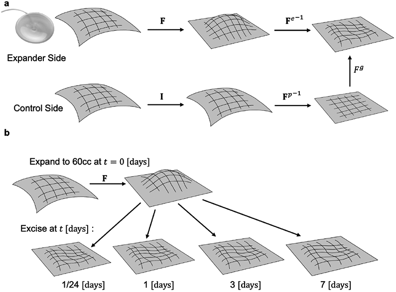
Finite volume growth framework. a) The deformation induced by the expander in vivo is the total deformation F. Upon excision, the skin deforms elastically according to Fe. On the control side, there is no deformation in vivo and the map is the identity I. Upon excision of the control path the prestrain deformation Fp can be calculated. Comparison between the ex vivo expanded and control patches is used to estimate the growth Fg. b) To quantify the dynamics of skin growth, a single inflation volume of 60 cc was applied at the time t = 0 [days] and the skin excised at times t = [1/24, 1, 3, 7] [days].
The split of the deformation gradient into growth and elastic contributions is akin to plasticity. In previous work, we have considered area growth as a transversely isotropic process [19], in such case the growth tensor can be expressed as
| (3) |
where N is the normal to the skin surface, Is = I − N ⊗ N is the surface identity, and ϑg is a scalar variable called the growth multiplier which represents the total area growth. However, in view of anisotropic properties of skin [27, 28], we also introduce an anisotropic growth tensor
| (4) |
where now there are two growth variables and describing the growth in each of the directions, longitudinal and transverse. In this case the total area growth is given by their product . In both Eqs. (3) and (4) the growth tensor neglects permanent changes in thickness [26]. In the following sections, we work with both isotropic and anisotropic growth tensors and fit both of these models to the data in order to determine the extent to which isotropy is a valid assumption or if anisotropic models are needed.
Having introduced the split in Eq. (2), the evolution of the state of stress and deformation as well as the change in growth require clarification of the constitutive equations. Growth is a biological process which is complex and noisy, dictated by the interaction of several cell signaling networks [29, 30, 31, 32, 21]. We simplify our mathematical model with a phenomenological growth law in which the growth rate is linearly proportional to the elastic deformation. This idealization is introduced based on our overall understanding that stretch triggers growth, while avoiding the complex biological processes that take place during growth. For the case of the total area growth in the transversely isotropic case we have
| (5) |
with ϑe = ∣cof(Fe) · N∣ the elastic area change, and ϑcrit a critical value of elastic stretch beyond which there is growth . The operator cof(●) is the cofactor. For the anisotropic case we have two constitutive equations, one for each of the growth multipliers, which take on the same form as Eq. (5),
| (6) |
with the elastic stretch along the Gα direction, and the critical stretch beyond which growth occurs. Having specified the growth component, the deformation of the tissue is given by the standard linear momentum balance condition ∇ · σ = 0. The stress, in turn, depends on the elastic deformation Fe through the appropriate constitutive equations, as described next.
Mechanical behavior of skin
We consider that skin behaves as a hyperelastic material with strain energy Ψ, and the state of stress depends solely on the elastic deformation Fe through the left Cauchy-Green deformation tensor be = Fe · FeT and the volume change Je = det Fe,
| (7) |
Two constitutive models are used to describe skin’s mechanical response. Considering the tissue as isotropic, a neo-Hookean strain energy density function is used [18, 25],
| (8) |
is the first invariant of be, and μ and λ are Lame parameters. Alternatively, we also employ an anisotropic strain energy density function proposed originally by Gasser, Ogden and Holzapfel (GOH) for arteries but used successfully to capture skin mechanical behavior [33, 22, 34],
| (9) |
The symbol ⟨●⟩ denotes the Macaulay brackets. The generalized fiber strain is defined as
| (10) |
with the first isochoric invariant of be, and the isochoric portion of the fiber stretch. The fiber stretch is a pseudoinvariant since it depends on the choice of material direction a0 in the reference configuration, which gets mapped to a = Fe · a0 upon deformation, or, if only the isochoric deformation is used, where . The parameters of the GOH model include the Lame constants for the isotropic contributions plus three new parameters to describe anisotropy, kc, a, and κ. The GOH model is one of multiple anisotropic hyperelastic potentials capable of describing skin’s mechanical behavior [28]. The GOH model has limitations, such as the use of the homogenized structural tensor as opposed to integration of individual fiber contributions over the unit sphere [35, 36, 37]. Additionally, the GOH model has been the focus of significant debate regarding the use of the Macaulay brackets for the generalized fiber strain. Even though the assumption that fibers under compression do not contribute to the energy is reasonable, the generalized fiber strain in eq. (10) does not isolate fiber strains and could lead to material behavior that is not observed experimentally [38, 39, 40]. However, we use the GOH model due to its simplicity and computational efficiency, together with its ability to capture the biaxial behavior of skin such as expected here [41].
Finite element implementation
Details about the implementation of the isotropic model (transversely isotropic growth with neo-Hookean material) are available in our previous work [18, 25]. However, for the current work we have implemented the anisotropic growth with the anisotropic strain energy density function, Eq. (9). The code is available with this publication and a few clarifications are introduced here. The spatial elasticity tensor corresponding to the Oldroydrate of the Kirchhoff stress has both an elastic and a growth component
| (11) |
The first term, , is the standard elasticity tensor for large deformation hyperelasticity. The second term, , reflects the change in stress due to growth. The spatial elasticity tensor can be obtained through the push-forward operation of the Lagrangian counterpart , as shown in Eq. (11), or directly in the spatial configuration, e.g. [42, 43]. Eq. (11) also introduced the following outer product . Since the growth function itself is a function of the deformation, the form of depends on the choice of both the material model and the growth function [44, 45]. For the anisotropic growth model in Eq. (6), the relationship is
| (12) |
where gα = F · Gα are the push forward of the vectors specifying the longitudinal and transverse axes in the reference configuration, with corresponding total stretches . The stress and tangent tensors are coded into a user material subroutine (UMAT) in the commercial finite element package Abaqus (3DS, Waltham, USA).
The calibrated growth Eqs. (5) and (6) are used in a finite element simulation in our UMAT subroutine in order to do uncertainty propagation at the tissue level. The setup of the simulation is illustrated in Fig. 3. The domain is a square patch of tissue of 10 × 10 [cm2] discretized with 800 linear hexahedral elements C3D8 (20×20 elements in plane, and 2 elements across the thickness). The normal to the skin surface in the finite element simulations is the vector N = [0, 0, 1]⊤. Underneath the tissue, a rectangular expander of 4 × 6 [cm2] is placed, following the animal protocol and the manufacturer specification. The expander is discretized with 144 quadrilateral shell elements. The material model for the expander is hyperelastic neo-Hookean with parameters (as defined in the Abaqus input file) C10 = 0.436 MPa and D1 = 0.013 MPa−1. Note that the Abaqus definition of these parameters are related to the more commonly encountered neo-Hookean parameters C10 = μ/2 and D1 = 6/(3λ + 2μ), with μ and λ the Lame constants. Fluid cavity elements are used inside the expander. Fixed boundary conditions are applied at the bottom surface of the skin patch in a region surrounding the expander. These boundary conditions are based on the fact that skin is attached to the underlying muscle and that a pocket is created by separating the skin from the fascia in order to place the expander [46, 47]. For instance, Figure 1b depicts a 3D picture of a patch of skin that has been expanded, showing that the deformation is mostly limited to the region in which the skin was detached from the underlying fascia . Contact between the expander and the skin is assumed frictionless since smooth expanders were used in the experiments. The effect of friction is investigated in the Supplementary Material. A user defined amplitude function (UAMP) is used to control the inflation volume. At the start of the simulation, the expander is inflated to the target volume of 60 cc and no growth is allowed. Once the expander reaches the target volume, the growth model is enabled and the model runs for 7 days of simulated time. Fig. 3 shows the setup of the simulation, as well as an example of the total deformation ϑ and the end of the inflation step.
Figure 3:

Finite element model of tissue expansion. A rectangular domain of 10×10 [cm2] is discretized with 800 hexahedral elements. A 4 × 6 [cm2] expander, discretized with 676 quadrilateral shell elements, is placed underneath. A fluid cavity is used to inflate the expander to the desired volume. The second panel shows the total area stretch ϑ at the end of the inflation step, before growth, for a typical simulation. The tissue is characterized by its anisotropic mechanical behavior, described in terms of the vectors G1 and G2, which correspond to the longitudinal and transverse anatomical axes respectively.
Bayesian parameter calibration
For every expanded skin patch, the data are 10 × 10 arrays containing the tensors F, Fp, Fe, Fg. The goal of the inference problem is to learn the distribution of the parameters in Eqs. (5) and (6) that best describe the data. We remark that the data shows a high variance, inherent to the biological process and also a consequence of the inherent variability of a large animal protocol spanning several days in which the animals continue their normal routine. Therefore, we opt for a fully Bayesian approach to deal with these uncertainties.
For the isotropic growth case, Eq. (5), we start by posing a prior over the parameter p(kϑ) and an independent prior over the measurement noise p(s). A reasonable prior for the rate parameter is always positive so we use a log-normal distribution log(k) ~ N(−4, 0.5) while for the measurement error we use a Gamma distribution as prior σ ~ Γ(3,0.05). The data is arranged as D = (x, y) with inputs x = (ϑ, ϑp) and output y = ϑg. The average of prestrain across all skin patches is used as ϑcrit. For a given value of the parameters and for a given input x ∈ D, the ODE in Eq. (5) is integrated numerically to predict the output . The comparison of the prediction and the observed data y ∈ D is used to define the likelihood for a particular choice of parameters z*,
| (13) |
where ϑg is the mean and s is the variance of the likelihood distribution. Using Bayes’ rule, the posterior of the parameters is proportional to the product of the prior and the likelihood,
| (14) |
We sample from this posterior distribution using the sequential Monte Carlo sampling scheme available in PyMC3, a probabilistic programming module in Python [48]. We also sample the posterior distribution of the measurement noise, p(s∣D). Posteriors for the noise are not further discussed in the main text but available in the Supplementary Material. Additionally, it should be remarked that only the rate parameter in Eq. (5) is calibrated, but not the critical stretch ϑcrit. The critical stretch ϑcrit is set equal to the prestrain value ϑp = ∣cof(Fp) · N∣. This constraint on the critical stretch is needed to satisfy the homeostatic physiological state. This approach is similar to the methodology proposed by Costabal et al. [23].
A similar approach is used to infer the anisotropic rate parameters that were introduced in Eq. (6). The critical stretches for the anisotropic growth equations are also constrained based on the prestrain measurements, , .
Uncertainty propagation through the finite element model
Once the parameters of the growth constitutive model have been inferred from the point-wise data, we use the finite element model to compute the deformation and growth fields at the whole tissue scale. Instead of running a single deterministic simulation for the finite element model, we evaluate the finite element model multiple times by sampling from the posterior distribution of the biological parameters p(z∣D). Moreover, uncertainty in other parameters of the finite element model are also considered. We assume that the parameters of the mechanical constitutive Eqs. (8) and (9) are also uncertain and we sample these material properties from distributions based on our previous work [22, 25]. For the isotropic model we consider mean parameters , , and assume a uniform distribution around these parameters such that μ ∈ [0.666, 0.814] MPa, λ ∈ [0.4896, 0.544] MPa. For the anisotropic growth model we consider μ = 0.05 MPa, kc = 0.24 MPa, a = 2.88. The directions G1, G2 are not only aligned with the anatomical axes in the animal, but in fact correspond to the directions of skin anisotropy due to collagen fiber alignment in dorsal porcine skin [49]. The transverse direction, G2, is stiffer [49]. Thus, the fiber family in the GOH model is aligned with the transverse axis, a0∥G2, and has a dispersion κ = 0.0498. Variation in kc and μ is considered, such that kc ∈ [0.216, 0.264] MPa, and μ ∈ [0.045, 0.055] MPa according to [22]. Finally, to account for variation in the protocol, we also consider small variations to the inflation volume and the region over which the boundary conditions are applied.
Results
Deformation and growth in the porcine model
Upon expander inflation, the region near the apex of the expander undergoes the largest deformation in all cases. The average total area change ϑ is shown in Fig. 4a. Note that due to the expander being in different locations in different patches across the different animals, the average contour in Fig. 4a actually underestimates the total area change, but shows clearly that greater deformations occur at the apex of the expander and decrease toward the periphery. We remark that the field ϑ is the contour of relative area change between the initial in vivo skin before tissue expansion, and the skin patch also in vivo, after expansion, but before sacrifice. The average prestrain ϑp, which is measured on the control (not expanded) patches is more uniform, with a slight increase in prestrain toward the ventral side of the animal compared to the dorsal line, see Fig. 4b. The growth contours ϑg for the different time points are illustrated in Fig. 4c. Growth, which is the relative change in area with respect to the control patch, increases over time following tissue expansion. Additionally, the growth contour gradually resembles the total deformation. In other words, at the 7-day time point the growth field ϑg is greater at the apex and less toward the periphery of the expanded region. The elastic deformation field ϑe is the amount of elastic recoil or shrinking of the expanded patches once they are excised from the animal. The field ϑe resembles the total area change at 1 hour, but gradually decreases in magnitude and becomes more uniform as time progresses. These findings align with our previous observations and justify the growth model in Eq. (5) in which growth rate is assumed proportional to elastic deformation at a given time [13, 20].
Figure 4:

a) Total area changes due to tissue expansion for N=6 patches inflated to 60cc. The average of the total deformation ϑ measures the area changes from the in vivo skin before expansion to the in vivo skin patch after expansion and before sacrifice. The contour ϑ is greater at the expander apex and decreases toward the periphery of the expanded region. b) The prestrain field ϑp is determined from the N=6 control patches. c) The growth contour ϑg measures the permanent changes in area over time, and shows increasing area growth that resembles the expander placement. d) The elastic stretch contours ϑe measure the elastic recoil or shrinkage of skin patches after they are excised from the animal. e) The contours are all referred to the same parent domain, which entails mirroring of some of the patches with respect to the longitudinal axis of the animal. The direction G1 depicted in the contour plots is aligned with the longitudinal (rostral-caudal) axis, while G2 is aligned with the transverse (dorsal-ventral) axis.
Skin tissue is anisotropic due to the presence of a collagen network in the dermis, the load bearing layer of the skin [50]. In the swine, the collagen network in the skin has a preferred orientation in the transverse direction [51, 49, 52]. To measure the anisotropic skin deformation during tissue expansion, we decomposed the area changes into the stretches in the directions G1 and G2. The vector G1 denotes the caudal-rostral axis; G2 is the transverse orientation, dorsal to ventral. In Fig. 5a we observe that the average total deformation λ1 is greater than the average total deformation λ2 shown in Fig. 5c. This agrees with the knowledge of the direction of anisotropy in the swine. In contrast, the prestrain is greater on average in the transverse direction, as illustrated in Figs. 5b and d. The growth contours for the two directions of interest offer less clear trends compared to the total area change. This reflects the amount of variability across different skin patches, which gets exacerbated when the deformation is decomposed into contours with overall smaller values. Nevertheless, the rostral-caudal axis shows growth contours that increase over time in a similar manner to the total area growth, see in particular Fig. 5e.
Figure 5:

Anisotropic deformation due to tissue expansion. The total area deformation induced by the tissue expander is separated into the caudal-rostral axis component λ1 (a), and the transverse axis component λ2 (b). Longitudinal deformations λ1 are greater than the transverse deformations λ2. Prestrain is greater in the transverse direction (c,d). Growth increases over time. The growth in the longitudinal direction, (e), is greater than the growth in the transverse direction (g). Residual elastic deformation exists on expanded patches after excision from the animal (f,h).
Bayesian calibration of growth parameters
Undoubtedly, the data from this biological system reveals the inherent variability in skin mechanics and biological adaptation across different animals and skin regions. Additionally, other sources of uncertainty include the fact that the expanders are not completely fixed in place, but rather they move relative to the grid because the animals are free to move and interact with each other throughout the duration of the protocol. Nevertheless, following our hypothesis that the data could be explained by our mathematical model, we pooled all the data points (from each square in the 10 × 10 grid of each patch and for all time points) and ran our Bayesian inference code. The result of the inference for the isotropic growth model is shown in Fig. 6a. The variability in the data leads to a distribution of the growth parameter k in the range [0.02, 0.08] hr−1, with median k = 0.0453hr−1. Fig. 6b shows the evolution of the growth variable ϑg over time for three locations: apex, intermediate, and peripheral points in the expanded patch. The solid points are experimental data and the shaded regions denote the 90 percent confidence interval estimated from the model. Note that the curves in Fig. 6b are obtained by integrating the Eq. (5) directly. However, as described in the Methods, we then sampled from the posterior p(k∣D) and incorporated also the material behavior uncertainty in the finite element model. The result is shown in Fig. 6c. The trends are similar between the direct integration of the differential equation and the finite element simulation. Even though growth is directly linked to the elastic deformation through Eq. (5), in the clinical setting the surgeon can only control the total deformation. Thus, understanding the relationship between total deformation and growth is relevant for the clinical application even if growth is not directly explained by the total deformation in the mathematical model. Therefore, an independent relationship between total deformation and growth is shown in the Supplementrary Material.
Figure 6:

Bayesian inference of the growth parameter in the isotropic growth model. a) The posterior of the growth rate parameter k. b) Integration of Eq. (5) when sampling from the posterior of k for three different locations in the expanded patch. c) Growth over time for three different locations in the expanded patch predicted by the finite element model taking into consideration the uncertain growth parameter as well as material properties.
Figs. 7 and 8 show the result of the inference for the growth parameters k1 and k2. Similar trends to the total area change are observed. The growth rate for the longitudinal direction, kl, has a slightly wider distribution compared to the growth rate in the isotropic case. The growth rate in the longitudinal direction is in the range k1 ∈ [0.05, 0.1] hr−1 with median k1 = 0.0637 hr−1. The fact that in the longitudinal direction there is a greater speed of adaptation compared to the overall area growth rate is balanced by the growth rate in the transverse direction, k2, which is in the range k2 ∈ [0.01, 0.05] hr−1, with median k1 = 0.03 hr−1. The different speed of adaptation in the two directions is further observed in Figs. 7b and 8b, which plot the integration of Eq. (6) for three different locations, the apex of the expander, an intermediate point, and a point in the periphery. The shaded area in the plot denotes the 90 percent confidence interval inferred by the Bayesian calibration. Growth is more gradual in Fig. 8b compared to 7b. The growth at the apex is greater compared to the points in the middle and periphery of the expanded area for both directions. These trends are maintained through the finite element simulations.
Figure 7:

Bayesian inference of the growth parameter k1. a) Posterior distribution of the growth rate k1 which describes the biological adaptation in the longitudinal axis. b) Longitudinal growth over time for three locations of interest based on the direct integration of Eq. (6). c) Growth in the longitudinal direction over time from the finite element simulation of the anisotropic material with anisotropic growth model.
Figure 8:

Bayesian inference of the parameter k2, which describes the growth rate in the transverse direction. a) The posterior distribution of k2. b) Integration of the growth model Eq. (6) over time while sampling from the posterior distribution of k2. Three locations in the expanded region are shown. c) Growth in the transverse direction predicted by the finite element model.
Uncertainty propagation through the finite element model
The calibration of the growth rate parameters was performed with the point-wise data, using the ordinary differential Eqs. (5) and (6). The input to Eqs. (5) and (6) was the measured total deformation, ϑ, for the isotropic case, and λ1,λ2 for the anisotropic case. However, in the end, the process of tissue expansion involves the coupling of the biological process to the deformation of the tissue in response to the expander. Our goal is to have a calibrated finite element model that can predict the entire process, not just the biological response, but the deformation of the skin as well. Following the Methods, we created two finite element models, one for the isotropic case and one for the anisotropic case. We used the calibration from the previous section and sampled from the posterior of the growth parameters, p(k), p(k1) and p(k2) to evaluate the finite element models repeatedly.
Fig. 9 shows the results from the isotropic finite element model. In this case the tissue is modeled as neo-Hookean and the growth Eq. (5) is used at every integration point. The average deformation field ϑ shows a similar pattern to the experimental result. The deformation is greater at the apex and less toward the periphery. Over time, the growth field increases, and aligns with the total deformation, with greater growth at the apex and less toward the periphery. The elastic deformation obeys an inverse trend, similar to the experimental results depicted in Fig. 4. The curves in Fig. 9 further show that the total deformation at the apex stays constant over time since the expander is filled to 60 cc initially but then the volume is kept constant after inflation. Initially, all the deformation at the apex is elastic and there is no growth. Over time, growth increases as the elastic deformation decreases. The variability in the biological and material parameters propagated through the finite element model is depicted as shaded areas in Fig. 9. The solid lines in the plot of Fig. 9 correspond to the median parameters.
Figure 9:

Finite element simulation of tissue expansion when the skin is assumed as isotropic with growth also considered as isotropic. The total area change ϑ is greatest at the apex and less toward the periphery of the expanded region. Growth, ϑg increases over time, with greater growth at the center and less toward the periphery. The elastic deformation follows and inverse trend. This is further summarized with the plot on the bottom left, which shows the deformation, growth, and elastic deformation at the apex over time. The shaded area in the plot is achieved by sampling the uncertain biological and material parameters as described in the methodology. The solid curve in the plot corresponds to the median parameters.
The results from the anisotropic finite element model are shown in Fig. 10. We note that in these simulations there are two effects of anisotropy. First, the tissue is modeled as an anisotropic material based on Eq. (9). As a direct result of this difference in material properties, we observe that the average stretches in the longitudinal direction, λ1, are greater than the stretches in the transverse orientation, λ2. This aligns with the experimental data in Fig. 5. In addition to the anisotropy of the material, the biological response is also anisotropic. The growth Eq. (6) is used at every integration point, and the posterior of the growth rate for each direction, k1 and k2, are used. Additional uncertainty is captured by sampling the GOH parameters. Total, growth and elastic deformation for the longitudinal direction are shown in Fig. 10 left, while the corresponding contours in the transverse direction are shown in Fig. 10 right. The plots further show the distribution of total, elastic, and growth deformations for the apex obtained from multiple finite element simulations that sample the posterior of the biological and material parameters. Growth in the longitudinal direction, , increases more rapidly over the 7 days of the simulation compared to the transverse growth .
Figure 10:

Finite element model of anisotropic tissue expansion. There are two sources of anisotropy. First, the tissue is anisotropic, with preferred fiber orientation G2. As a result, the total deformation in the longitudinal direction, λ1, is greater than the total transverse deformation λ2. Growth is also anisotropic, with characteristic rates k1 > k2. As a result, growth in the longitudinal axis, , increases more rapidly than transverse growth . Spatially, growth is greater in the apex and less toward the periphery in both directions. Plots of total, elastic, and growth deformation over time for the apex point show the variance in the finite element simulation captured as a shaded area, which is the result from multiple simulations that sample biological and material parameter distributions. Solid lines in the plots correspond to the median parameters.
Discussion
In this work we present for the first time the calibration of a finite element model of skin growth to experimental data from a large animal model of tissue expansion. We find that the area change has a rate constant k ∈ [0.02, 0.05] hr−1. The growth process is anisotropic, with greater adaptation in the longitudinal axis of the animal compared to the transverse axis. The rate constant for the longitudinal axis is k1 ∈ [0.04, 0.1] hr−1, while for the transverse direction we find k2 ∈ [0.01, 0.05] hr−1. The anisotropy in the biological response is aligned with the anisotropic mechanical response of porcine’s dorsal skin, which is characterized by a preferred collagen orientation and stiffer behavior in the transverse direction [51, 49]. The calibrated finite element model quantitatively explains both the spatial variations in growth due to the nonlinear mechanics of the expander-skin system, as well as the time scale of skin’s biological adaptation. Additionally, through a Bayesian framework, we estimated the uncertainty in this system, which we can propagate through the finite element simulations. Thus, our computational model can now be used to design better expanders and tissue expansion protocols that lead to the desired amount and shape of skin growth. We expect that our work will have imminent utility in clinical practice.
The constitutive Eqs. (5) and (6) are able to describe the increase in growth over time as well as the spatial variation in growth due to the spatial variation in deformation. These equations are based on extensive evidence that growth is proportional to stretch [32, 21, 53]. This model also follows other recent efforts to describe the growth and remodeling of soft tissues, including our previous work on skin [25], as well as a vast literature on soft tissue growth [54, 55, 56]. The underlying mechanobiology is much more complex, and a detailed model based on a systems biology approach can provide further insight into the dynamics of this process, see for example recent efforts in heart mechanobiology modeling [57, 58]. Nevertheless, a key appeal of our approach is that we are able to condense the biological adaptation to three rate parameters that can be informed by the experimental data, enabling a quantitative understanding of the dynamics of skin mechanobiology in tissue expansion.
Our previous work with the porcine model of tissue expansion has motivated the development of finite element models to capture the spatio-temporal adaptation of skin. The spatio-temporal variation in total, growth, and elastic deformations follows from the coupling of the nonlinear mechanics of the skin expansion process with the biological adaptation of skin [13, 20, 26]. Here, we calibrate a finite element model to quantitatively explain the experimental observations. The calibration is done with a Bayesian approach to deal with the inherent uncertainties of the protocol. With the Bayesian calibration step we are able to obtain unimodal posteriors of the growth rate parameters, see Figs. 6-8. This implies that despite the uncertainty, the computational model is able to capture clear trends in the data. Together, the data and successful calibration of the parameters further suggest that spatio-temporal growth of skin in tissue expansion can be explained and predicted by our finite element framework. Importantly, we extended the framework with respect to our previous work [13] to include anisotropic material behavior and anisotropic growth. The data (Fig. 5), calibration results (Figs. 7,8), and existing evidence of skin anisotropy [51, 49], further support the need for anisotropic finite element models of tissue expansion. The finite element simulations can be further refined to capture the more complex interaction of the tissue with the underlying tissues, more realistic geometries, as well as contact between expander and skin. This is part of our ongoing work.
There are limitations to our current work that can be improved in the future. First of all, as we anticipated, small variations in the protocol can lead to a large variance in the data [25]. In particular, the calibration step assumes that the expander is fixed in place. Movement of the expander underneath the grid is, however, unavoidable. This means that the deformation of a particular grid location is not constant over time. A potential solution to this limitation is to develop new protocols to measure the deformation continuously. This is a challenging problem because we must avoid undue stress to the animals. Despite the movement, the process is repeatable. More importantly, we can quantify the uncertainty and make predictions including confidence intervals. While not guaranteed to narrow down the confidence intervals, more experimental data will help calibrate the model over a wider input space. In this work we have focused on a single inflation step of 60 cc. Future work will explore the effect of multiple inflation steps and different volumes to match a more representative set of clinical protocols [59, 20]. The growth equations (5) and (6) are simple models linking stretch to growth. More nonlinear models of tissue growth have been explored in the past, including for skin [60, 43], but with little biological basis. For example, previous models included dependence of the growth rate on the current amount of growth. These models have no biological basis since the growth amount depends on the reference configuration which is arbitrary. In a previous paper [25], we proposed the use of Hill equations. While still phenomenological, the equation proposed in [25] considered that biological network interactions are accurately modeled through Hill functions, including systems biology models of tissue growth [61, 58]. However, even though a slightly more mechanistic framework, the fits to the Hill function growth equation were not necessarily any better than with the simpler models. A more thorough discussion of the performance of the Hill function growth rate models is documented in the Supplementary Material. Lastly, we have quantified the anisotropic growth of skin in tissue expansion, but a detailed characterization of the mechanical behavior of skin and how it changes due to tissue expansion is an ongoing effort. Without specific knowledge of the exact distribution of material parameters, we opted for a uniform distribution for the material parameters [62]. Nevertheless, future work is needed to better model the material behavior uncertainty. Based on our knowledge of the anisotropy of skin [49, 52], we have improved our previous computational models which treated skin as isotropic [25]. The new framework captures anisotropic growth and anisotropic mechanical response based on [33]. Yet, it also continues to consider skin as hyperelastic. Consideration of viscoelastic behavior, or even a poro-hyperviscoelastic framework would increase the fidelity of the model [63]. Also, while it has been reported that skin’s mechanical response does not change significantly due to growth [4, 64], more data is needed particularly in this regard. Finally, here we use the popular GOH model to describe skin biaxial mechanics [41]. However, in view of the limitations of this model [38, 40, 39], and the advances in data-driven approaches in computational mechanics, future work will avoid closed-form constitutive equations in favor of our recent developments on data-driven constitutive models of skin [65].
Conclusion
We have quantified the spatio-temporal dynamics of skin growth due to tissue expansion and used these data to calibrate a finite element model of skin growth. Model calibration was performed within a Bayesian framework in order to infer the rate constants of the biological process of skin growth including the role of uncertainty. With our combination of experiments, finite element modeling, and Bayesian calibration, we have now quantitative understanding of this process: area growth is proportional to stretch with rate constant of kin[0.02, 0.08]hr−1, and this process is anisotropic, with larger deformation and growth in the longitudinal axis of the animal (rostral-caudal), orthogonal to the preferred collagen orientation in the dorsal skin of the swine which is in the transverse direction. Together, our in vivo - in silico approach will enable the engineering design of tissue expansion protocols that minimize complications and achieve the desired shape and size of newly grown skin flaps.
Supplementary Material
Statement of Significance.
Tissue expansion is a widely used technique in reconstructive surgery because it triggers growth of skin for the correction of large skin lesions and for breast reconstruction after mastectomy. Despite of its potential, complications and undesired outcomes persist due to our incomplete understanding of skin mechanobiology. Here we quantify the deformation and growth fields induced by an expander over 7 days in a porcine animal model and use these data to calibrate a computational model of skin growth using finite element simulations and a Bayesian framework. The calibrated model is a leap forward in our understanding skin growth, we now have quantitative understanding of this process: area growth is anisotropic and it is proportional to stretch with a characteristic rate constant of k ∈ [0.02,0.08]hr−1.
Acknowledgements
This work was supported by the National Institute of Arthritis and Musculoskeletal and Skin Diseases of the National Institute of Health under award R01AR074525.
Footnotes
Supplementary Material
Code and data for this publication are available at: https://github.com/abuganza/BayesianCalibrationSkinGrowth
Declaration of interests
The authors declare that they have no known competing financial interests or personal relationships that could have appeared to influence the work reported in this paper.
Publisher's Disclaimer: This is a PDF file of an unedited manuscript that has been accepted for publication. As a service to our customers we are providing this early version of the manuscript. The manuscript will undergo copyediting, typesetting, and review of the resulting proof before it is published in its final form. Please note that during the production process errors may be discovered which could affect the content, and all legal disclaimers that apply to the journal pertain.
References
- [1].Radovan C, Breast reconstruction after mastectomy using the temporary expander., Plastic and Reconstructive Surgery 69 (1982) 195–208. [DOI] [PubMed] [Google Scholar]
- [2].Rivera R, LoGiudice J, Gosain AK, Tissue expansion in pediatric patients, Clinics in plastic surgery 32 (2005) 35–44. [DOI] [PubMed] [Google Scholar]
- [3].Manders EK, Schenden MJ, Furrey JA, Hetzler PT, Davis TS, Graham W 3rd, Soft-tissue expansion: concepts and complications., Plastic and Reconstructive Surgery 74 (1984) 493–507. [DOI] [PubMed] [Google Scholar]
- [4].Austad ED, Pasyk KA, McClatchey KD, Cherry GW, Histomorphologic evaluation of guinea pig skin and soft tissue after controlled tissue expansion., Plastic and reconstructive surgery 70 (1982) 704–710. [DOI] [PubMed] [Google Scholar]
- [5].VanderKolk CA, McCann JJ, Mitchell GM, O’Brien BM, Changes in area and thickness of expanded and unexpanded axial pattern skin flaps in pigs, British journal of plastic surgery 41 (1988) 284–293. [DOI] [PubMed] [Google Scholar]
- [6].Gosain AK, Zochowski CG, Cortes W, Refinements of tissue expansion for pediatric forehead reconstruction: a 13-year experience, Plastic and reconstructive surgery 124 (2009) 1559–1570. [DOI] [PubMed] [Google Scholar]
- [7].Pamplona DC, Velloso RQ, Radwanski HN, On skin expansion, Journal of the mechanical behavior of biomedical materials 29 (2014) 655–662. [DOI] [PubMed] [Google Scholar]
- [8].Bozkurt A, Groger A, Odey D, Vogeler F, Piatkowski A, Fuchs PC, Pallua N, Retrospective analysis of tissue expansion in reconstructive burn surgery: evaluation of complication rates, Burns 34 (2008) 1113–1118. [DOI] [PubMed] [Google Scholar]
- [9].Chepla KJ, Gosain AK, Giant nevus sebaceus: definition, surgical techniques, and rationale for treatment, Plastic and reconstructive surgery 130 (2012) 296e–304e. [DOI] [PubMed] [Google Scholar]
- [10].Hassanein AH, Rogers GF, Greene AK, Management of challenging congenital melanocytic nevi: outcomes study of serial excision, Journal of pediatric surgery 50 (2015) 613–616. [DOI] [PubMed] [Google Scholar]
- [11].Bartell TH, Mustoe TA, Animal models of human tissue expansion., Plastic and reconstructive surgery 83 (1989) 681–686. [DOI] [PubMed] [Google Scholar]
- [12].Van Rappard J, Molenaar J, Van Doorn K, Sonneveld G, Borghouts J, Surface-area increase in tissue expansion., Plastic and reconstructive surgery 82 (1988) 833–839. [DOI] [PubMed] [Google Scholar]
- [13].Tepole AB, Gart M, Gosain AK, Kuhl E, Characterization of living skin using multi-view stereo and isogeometric analysis, Acta biomaterialia 10 (2014) 4822–4831. [DOI] [PMC free article] [PubMed] [Google Scholar]
- [14].Tepole AB, Gart M, Purnell CA, Gosain AK, Kuhl E, Multi-view stereo analysis reveals anisotropy of prestrain, deformation, and growth in living skin, Biomechanics and modeling in mechanobiology 14 (2015) 1007–1019. [DOI] [PMC free article] [PubMed] [Google Scholar]
- [15].Cowin SC, Tissue growth and remodeling, Annu. Rev. Biomed. Eng 6 (2004) 77–107. [DOI] [PubMed] [Google Scholar]
- [16].Tepole AB, Vaca EE, Purnell CA, Gart M, McGrath J, Kuhl E, Gosain AK, Quantification of strain in a porcine model of skin expansion using multi-view stereo and isogeometric kinematics, JoVE (Journal of Visualized Experiments) (2017) e55052. [DOI] [PMC free article] [PubMed] [Google Scholar]
- [17].Eskandari M, Kuhl E, Systems biology and mechanics of growth, Wiley Interdisciplinary Reviews: Systems Biology and Medicine 7 (2015) 401–412. [DOI] [PMC free article] [PubMed] [Google Scholar]
- [18].Tepole AB, Gosain AK, Kuhl E, Stretching skin: The physiological limit and beyond, International journal of non-linear mechanics 47 (2012) 938–949. [DOI] [PMC free article] [PubMed] [Google Scholar]
- [19].Tepole AB, Ploch CJ, Wong J, Gosain AK, Kuhl E, Growing skin: a computational model for skin expansion in reconstructive surgery, Journal of the Mechanics and Physics of Solids 59 (2011) 2177–2190. [DOI] [PMC free article] [PubMed] [Google Scholar]
- [20].Lee T, Vaca EE, Ledwon JK, Bae H, Topczewska JM, Turin SY, Kuhl E, Gosain AK, Tepole AB, Improving tissue expansion protocols through computational modeling, Journal of the mechanical behavior of biomedical materials 82 (2018) 224–234. [DOI] [PMC free article] [PubMed] [Google Scholar]
- [21].Aragona M, Sifrim A, Malfait M, Song Y, Van Herck J, Dekoninck S, Gargouri S, Lapouge G, Swedlund B, Dubois C, et al. , Mechanisms of stretch-mediated skin expansion at single-cell resolution, Nature 584 (2020) 268–273. [DOI] [PMC free article] [PubMed] [Google Scholar]
- [22].Lee T, Turin SY, Gosain AK, Bilionis I, Tepole AB, Propagation of material behavior uncertainty in a nonlinear finite element model of reconstructive surgery, Biomechanics and modeling in mechanobiology 17 (2018) 1857–1873. [DOI] [PubMed] [Google Scholar]
- [23].Costabal FS, Choy J, Sack KL, Guccione JM, Kassab G, Kuhl E, Multiscale characterization of heart failure, Acta biomaterialia 86 (2019) 66–76. [DOI] [PMC free article] [PubMed] [Google Scholar]
- [24].Peirlinck M, Costabal FS, Sack K, Choy J, Kassab G, Guccione J, De Beule M, Segers P, Kuhl E, Using machine learning to characterize heart failure across the scales, Biomechanics and modeling in mechanobiology (2019) 1–15. [DOI] [PubMed] [Google Scholar]
- [25].Lee T, Bilionis I, Tepole AB, Propagation of uncertainty in the mechanical and biological response of growing tissues using multi-fidelity gaussian process regression, Computer Methods in Applied Mechanics and Engineering 359 (2020) 112724. [DOI] [PMC free article] [PubMed] [Google Scholar]
- [26].Janes LE, Ledwon JK, Vaca EE, Turin SY, Lee T, Tepole AB, Bae H, Gosain AK, Modeling tissue expansion with isogeometric analysis: Skin growth and tissue level changes in the porcine model, Plastic and reconstructive surgery 146 (2020) 792–798. [DOI] [PubMed] [Google Scholar]
- [27].Jor JW, Parker MD, Taberner AJ, Nash MP, Nielsen PM, Computational and experimental characterization of skin mechanics: identifying current challenges and future directions, Wiley Interdisciplinary Reviews: Systems Biology and Medicine 5 (2013) 539–556. [DOI] [PubMed] [Google Scholar]
- [28].Limbert G, Mathematical and computational modelling of skin biophysics: a review, Proceedings of the Royal Society A: Mathematical, Physical and Engineering Sciences 473 (2017) 20170257. [DOI] [PMC free article] [PubMed] [Google Scholar]
- [29].Yang M, Liang Y, Sheng L, Shen G, Liu K, Gu B, Meng F, Li Q, A preliminary study of differentially expressed genes in expanded skin and normal skin: implications for adult skin regeneration, Archives of dermatological research 303 (2011) 125–133. [DOI] [PubMed] [Google Scholar]
- [30].Zhou S-B, Wang J, Chiang C-A, Sheng L-L, Li Q-F, Mechanical stretch upregulates sdf-1α in skin tissue and induces migration of circulating bone marrow-derived stem cells into the expanded skin, Stem Cells 31 (2013) 2703–2713. [DOI] [PubMed] [Google Scholar]
- [31].Liang X, Huang X, Zhou Y, Jin R, Li Q, Mechanical stretching promotes skin tissue regeneration via enhancing mesenchymal stem cell homing and transdifferentiation, Stem cells translational medicine 5 (2016) 960–969. [DOI] [PMC free article] [PubMed] [Google Scholar]
- [32].Razzak MA, Hossain M, Radzi ZB, Yahya NAB, Czernuszka J, Rahman MT, Cellular and molecular responses to mechanical expansion of tissue, Frontiers in physiology 7 (2016) 540. [DOI] [PMC free article] [PubMed] [Google Scholar]
- [33].Gasser TC, Ogden RW, Holzapfel GA, Hyperelastic modelling of arterial layers with distributed collagen fibre orientations, Journal of the royal society interface 3 (2006) 15–35. [DOI] [PMC free article] [PubMed] [Google Scholar]
- [34].Annaidh AN, Bruyère K, Destrade M, Gilchrist MD, Otténio M, Characterization of the anisotropic mechanical properties of excised human skin, Journal of the mechanical behavior of biomedical materials 5 (2012) 139–148. [DOI] [PubMed] [Google Scholar]
- [35].Menzel A, Harrysson M, Ristinmaa M, Towards an orientation-distribution-based multi-scale approach for remodelling biological tissues, Computer methods in biomechanics and biomedical engineering 11 (2008) 505–524. [DOI] [PubMed] [Google Scholar]
- [36].Alastrué V, Martinez M, Doblaré M, Menzel A, Anisotropic microsphere-based finite elasticity applied to blood vessel modelling, Journal of the Mechanics and Physics of Solids 57 (2009) 178–203. [Google Scholar]
- [37].Tonge TK, Voo LM, Nguyen TD, Full-field bulge test for planar anisotropic tissues: Part ii–a thin shell method for determining material parameters and comparison of two distributed fiber modeling approaches, Acta biomaterialia 9 (2013) 5926–5942. [DOI] [PubMed] [Google Scholar]
- [38].Volokh KY, On arterial fiber dispersion and auxetic effect, Journal of biomechanics 61 (2017) 123–130. [DOI] [PubMed] [Google Scholar]
- [39].Latorre M, Montáns FJ, On the tension-compression switch of the gasser–ogden–holzapfel model: Analysis and a new pre-integrated proposal, Journal of the mechanical behavior of biomedical materials 57 (2016) 175–189. [DOI] [PubMed] [Google Scholar]
- [40].Holzapfel GA, Ogden RW, On the tension–compression switch in soft fibrous solids, European Journal of Mechanics-A/Solids 49 (2015) 561–569. [Google Scholar]
- [41].Meador WD, Sugerman GP, Story HM, Seifert AW, Bersi MR, Tepole AB, Rausch MK, The regional-dependent biaxial behavior of young and aged mouse skin: A detailed histomechanical characterization, residual strain analysis, and constitutive model, Acta biomaterialia 101 (2020) 403–413. [DOI] [PubMed] [Google Scholar]
- [42].Himpel G, Kuhl E, Menzel A, Steinmann P, et al. , Computational modelling of isotropic multiplicative growth, Comp Mod Eng Sci 8 (2005) 119–134. [Google Scholar]
- [43].Zöllner AM, Holland MA, Honda KS, Gosain AK, Kuhl E, Growth on demand: reviewing the mechanobiology of stretched skin, Journal of the mechanical behavior of biomedical materials 28 (2013) 495–509. [DOI] [PMC free article] [PubMed] [Google Scholar]
- [44].Göktepe S, Abilez OJ, Parker KK, Kuhl E, A multiscale model for eccentric and concentric cardiac growth through sarcomerogenesis, Journal of theoretical biology 265 (2010) 433–442. [DOI] [PubMed] [Google Scholar]
- [45].Göktepe S, Abilez OJ, Kuhl E, A generic approach towards finite growth with examples of athlete’s heart, cardiac dilation, and cardiac wall thickening, Journal of the Mechanics and Physics of Solids 58 (2010) 1661–1680. [Google Scholar]
- [46].Raposio E, Nordström R, Santi P, Undermining of the scalp: quantitative effects., Plastic and reconstructive surgery 101 (1998) 1218–1222. [DOI] [PubMed] [Google Scholar]
- [47].Boyer JD, Zitelli JA, Brodland DG, Undermining in cutaneous surgery, Dermatologic surgery 27 (2001) 75–78. [PubMed] [Google Scholar]
- [48].Salvatier J, Wiecki TV, Fonnesbeck C, Probabilistic programming in python using PyMC3, PeerJ Computer Science 2 (2016) e55. [DOI] [PMC free article] [PubMed] [Google Scholar]
- [49].Pissarenko A, Yang W, Quan H, Brown KA, Williams A, Proud WG, Meyers MA, Tensile behavior and structural characterization of pig dermis, Acta biomaterialia 86 (2019) 77–95. [DOI] [PubMed] [Google Scholar]
- [50].Benítez JM, Montáns FJ, The mechanical behavior of skin: Structures and models for the finite element analysis, Computers & Structures 190 (2017) 75–107. [Google Scholar]
- [51].Ottenio M, Tran D, Annaidh AN, Gilchrist MD, Bruyère K, Strain rate and anisotropy effects on the tensile failure characteristics of human skin, Journal of the mechanical behavior of biomedical materials 41 (2015) 241–250. [DOI] [PubMed] [Google Scholar]
- [52].Lakhani P, Dwivedi KK, Kumar N, Directional dependent variation in mechanical properties of planar anisotropic porcine skin tissue, Journal of the mechanical behavior of biomedical materials 104 (2020) 103693. [DOI] [PubMed] [Google Scholar]
- [53].Ledwon JK, Kelsey LJ, Vaca EE, Gosain AK, Transcriptomic analysis reveals dynamic molecular changes in skin induced by mechanical forces secondary to tissue expansion, Scientific reports 10 (2020) 1–14. [DOI] [PMC free article] [PubMed] [Google Scholar]
- [54].Emmert MY, Schmitt BA, Loerakker S, Sanders B, Spriestersbach H, Fioretta ES, Bruder L, Brakmann K, Motta SE, Lintas V, et al. , Computational modeling guides tissue-engineered heart valve design for long-term in vivo performance in a translational sheep model, Science Translational Medicine 10 (2018). [DOI] [PubMed] [Google Scholar]
- [55].Ambrosi D, Ben Amar M, Cyron CJ, DeSimone A, Goriely A, Humphrey JD, Kuhl E, Growth and remodelling of living tissues: perspectives, challenges and opportunities, Journal of the Royal Society Interface 16 (2019) 20190233. [DOI] [PMC free article] [PubMed] [Google Scholar]
- [56].Latorre M, Modeling biological growth and remodeling: contrasting methods, contrasting needs, Current Opinion in Biomedical Engineering 15 (2020) 26–31. [Google Scholar]
- [57].Latorre M, Humphrey J, Numerical knockouts–in silico assessment of factors predisposing to thoracic aortic aneurysms, PLoS computational biology 16 (2020) e1008273. [DOI] [PMC free article] [PubMed] [Google Scholar]
- [58].Yoshida K, Holmes JW, Computational models of cardiac hypertrophy, Progress in Biophysics and Molecular Biology 159 (2021) 75–85. [DOI] [PMC free article] [PubMed] [Google Scholar]
- [59].Gosain AK, Turin SY, Chim H, LoGiudice JA, Salvaging the unavoidable: A review of complications in pediatric tissue expansion, Plastic and reconstructive surgery 142 (2018) 759–768. [DOI] [PubMed] [Google Scholar]
- [60].Lubarda VA, Hoger A, On the mechanics of solids with a growing mass, International journal of solids and structures 39 (2002) 4627–4664. [Google Scholar]
- [61].Frank DU, Sutcliffe MD, Saucerman JJ, Network-based predictions of in vivo cardiac hypertrophy, Journal of molecular and cellular cardiology 121 (2018) 180–189. [DOI] [PMC free article] [PubMed] [Google Scholar]
- [62].Madireddy S, Sista B, Vemaganti K, Bayesian calibration of hyperelastic constitutive models of soft tissue, Journal of the mechanical behavior of biomedical materials 59 (2016) 108–127. [DOI] [PubMed] [Google Scholar]
- [63].Sachs D, Wahlsten A, Kozerke S, Restivo G, Mazza E, A biphasic multilayer computational model of human skin, Biomechanics and modeling in mechanobiology 20 (2021) 969–982. [DOI] [PMC free article] [PubMed] [Google Scholar]
- [64].Zeng Y-J, Xu C-Q, Yang J, Sun G-C, Xu X-H, Biomechanical comparison between conventional and rapid expansion of skin, British journal of plastic surgery 56 (2003) 660–666. [DOI] [PubMed] [Google Scholar]
- [65].Tac V, Sree VD, Rausch MK, Tepole AB, Data-driven modeling of the mechanical behavior of anisotropic soft biological tissue, arXiv preprint arXiv:2107.05388 (2021). [DOI] [PMC free article] [PubMed] [Google Scholar]
Associated Data
This section collects any data citations, data availability statements, or supplementary materials included in this article.