Detection of abnormal left ventricular geometry in patients without cardiovascular disease through machine learning: An ECG‐based approach

Abstract

Cardiac remodeling is recognized as an important aspect of cardiovascular disease (CVD) progression. Machine learning (ML) techniques were applied to basic clinical parameters and electrocardiographic features, in order to detect abnormal left ventricular geometry (LVG) even before the onset of left ventricular hypertrophy (LVH), in a population without established CVD. The authors enrolled 528 patients with and without essential hypertension, but no other indications of CVD. All patients underwent a full echocardiographic evaluation and were classified into 3 groups; normal geometry (NG), concentric remodeling without LVH (CR), and LVH. Abnormal LVG was identified as increased relative wall thickness (RWT) and/or left ventricular mass index (LVMi). The authors trained supervised ML models to classify patients with abnormal LVG and calculated SHAP values to perform feature importance and interaction analysis. Hypertension, age, body mass index over the Sokolow‐Lyon voltage, QRS‐T angle, and QTc duration were some of the most important features. Our model was able to distinguish NG from CR+LVH combined, with 87% accuracy on an unseen test set, 75% specificity, 97% sensitivity, and area under the receiver operating curve (AUC/ROC) equal to 0.91. The authors also trained our model to classify NG and CR (NG + CR) against those with LVH, with 89% test set accuracy, 93% specificity, 67% sensitivity, and an AUC/ROC value of 0.89, for a 0.4 decision threshold. Our ML algorithm effectively detects abnormal LVG even at early stages. Innovative solutions are needed to improve risk stratification of patients without established CVD, and ML may enable progress in this direction.

We used machine learning techniques and found a combination of clinical and ECG features that enable prediction of abnormal left ventricular geometry or left ventricular hypertrophy (LVH). Concentric remodeling appears to be separable from LVH through a random forest method.

1. INTRODUCTION

The application of machine learning (ML) algorithms in the management of data are transforming the landscape of different scientific fields, including clinical medicine. ¹ ML has the potential to radically change the way we practice cardiovascular medicine by providing new tools for interpreting data and making clinical decisions. While still a new player in cardiology, ML has already made its mark in clinical diagnostics ² , ³ and research, ⁴ , ⁵ and continues to evolve rapidly. Physicians can leverage ML to make more accurate and prompt diagnoses, identify hidden opportunities to improve patient management, and avoid unnecessary spending.

Cardiac remodeling is an important aspect of cardiovascular disease (CVD) progression and is therefore emerging as a significant therapeutic target. ⁶ , ⁷ , ⁸ , ⁹ More specifically, arterial hypertension is associated with cardiac geometric adaptations that are matched to systemic hemodynamics and ventricular load, and have important prognostic implications. ⁶ , ⁷ , ⁸ , ⁹ Abnormal left ventricular geometry (LVG) in hypertensives is frequently associated with diastolic dysfunction, and left ventricular hypertrophy (LVH) is a major adverse prognostic risk factor for cardiovascular events. ¹⁰ , ¹¹ , ¹² The electrocardiogram (ECG), one of the most widely used diagnostic tools, is of paramount importance in the initial evaluation of a patient suspected to have a cardiovascular pathology. Nevertheless, the ECG is not a sensitive method for detecting LVH, and as far as we know, it cannot detect changes of LVG at early stages, especially before LVH is present. Notably, although the most commonly used ECG criteria demonstrate relatively high specificity, their sensitivity for the detection of LVH is low, approximately 30% ¹³ and in some studies, it is low as 6.9%. ¹⁴ For that reason, and given the importance of abnormal LVG, the echocardiogram is suggested as an additional diagnostic evaluation to hypertensive patients, according to the latest European guidelines for arterial hypertension. ¹⁵

The digital interpretation of ECG via computational methods and ML applications allows us to extract information that is not easily and directly detected by the human eye, especially within a busy clinical setting. On the other hand, echocardiography is a more sensitive approach for the detection of cardiac morphologic changes mediated by arterial hypertension, also more valuable for cardiovascular risk assessment. Nonetheless, it is debated whether echocardiography should be part of the diagnostic workup for all hypertensive patients, and its routine use in hypertensives is not endorsed by some hypertension societies. ¹⁶ It would therefore be ideal to expand the diagnostic capabilities of ECG in detecting hypertensive patients with left ventricular remodeling and LVH and refer them for further echocardiographic evaluation.

This study was designed to test the hypothesis that a 12‐lead ECG, a routine and inexpensive screening procedure, can provide further accuracy in detecting abnormal LVG, using ML methods, even at the early stages before the onset of LVH, in a population without established CVD. We also seek to understand which features contribute to the ML model's decisions, by calculating global feature importance and feature interactions.

2. METHODS

2.1. Study population

We carried out a cross‐sectional single‐center study from November 2019 to September 2020. We enrolled 528 consecutive patients, aged 30 years or older, with and without essential hypertension, but no indications of CVD. The diagnosis of hypertension was based on the recommendations of the European Society of Hypertension/European Society of Cardiology. ¹⁵

Patients with any of the following characteristics were excluded: pregnant or lactating women; secondary hypertension; tachy‐ or bradyarrhythmia; permanent atrial fibrillation; RBBB, LBBB or other conduction abnormalities of ECG; coronary artery disease, moderate or severe valvular heart disease, cardiomyopathy, cerebrovascular, liver or renal disease; history of acute coronary syndrome or myocarditis; ejection fraction <55%; history of drug or alcohol abuse; any chronic inflammatory or other infectious disease during the last 6 months; and thyroid gland disease. Vascular or neoplastic conditions were also ruled out. Weight and height were measured; using the World Health Organization (WHO) classification of body mass index (BMI), the individuals were classified into three groups: normal weight (18.5–24.9 kg/m²), overweight (25–29.9 kg/m²), and obese (≥30 kg/m²).

Functional tests for myocardial ischemia, coronary computed tomography angiography, or invasive coronary angiography were performed according to physician's judgment, in order to exclude coronary artery disease. The study was conducted in accordance with the Declaration of Helsinki, the protocol was approved by the Hospital Ethics Committee, and patients gave written informed consent to their participation in the study.

2.2. Echocardiography

A full echocardiographic study was blindly performed in all patients using a Vivid 7 (General Electric) ultrasound device according to the recommendations of the European Association of Cardiovascular Imaging and the American Society of Echocardiography ¹⁶ , ¹⁷ by two experienced echocardiographists. Abnormal LVG was identified as increased relative wall thickness (RWT) and/or left ventricular mass index (LVMi). Left ventricular hypertrophy was considered present if the LVMi was ≥115 g/m² and 95 g/m² for males and females, respectively. Relative wall thickness was defined as 2×PWT/LVIDd (LVIDd—left ventricular internal diastolic dimension, PWT—posterior wall thickness) using 2D measurements. ¹⁷ Normal RWT was defined as <0.43. ¹⁵

Patients were classified into 3 groups based on LVMi and RWT as follows: (a) NG, normal geometry, defined as normal LVMi and normal RWT, (b) CR, concentric remodeling, defined as normal LVMi and increased RWT, and (c) LVH, concentric hypertrophy or eccentric hypertrophy, defined as increased LVMi.

2.3. Electrocardiography

A 12‐lead ECG in the resting position with 10‐sec duration was performed on each patient using a digital 6‐Channel machine (Biocare iE 6) at the same visit with the echocardiographic study and was stored in XML format. Automated measurements were extracted from the digital files, using the Biocare software‐included package. These measurements were based on representative complexes of 1 s duration for each lead, produced by averaging over 10 s, and were verified and adjusted where needed. Using these representative complexes, additional measurements of amplitude and duration were obtained by our custom‐made code written in Python, ¹⁸ thus producing new features, explained below.

2.4. Feature engineering

Our Python code extracted additional ECG waveform measurements from the 1 s representative complex for each lead produced by the electrocardiograph. With the aid of automated measurements provided by the machine, we calculated several other predictors (features) such as areas under curves, slopes, and peak heights of curves (Table 1). ¹⁹

TABLE 1.

Clinical, anthropometric, and ECG data (features) used as inputs to the machine learning (ML) model

Feature	Description, Units/Classes	Range	Mean/Mode
Sex	Male/Female	2	F
Age	Age, years	31–90	61.5
Hypertension	History of hypertension*	2	1
BMI group	Body mass index class**	3	3
Height	Height, cm	137.0–194.0	165
BSA	Body surface area, m2	1.3–2.8	1.93
P duration	P wave duration, ms	0.0–154.0	113
QRS duration	QRS interval duration, ms	68.0–138.0	92.7
QTc duration	QT‐interval corrected for heart rate***, ms	368.0–510.0	422
ST duration	ST segment duration, ms	0.0–277.0	112
S amplitude (V1)	S wave amplitude in V1, mV	0.0–1.9	0.732
SL	Sokolow‐Lyon voltage, mV	0.5–4.5	1.93
R amplitude max	Tallest R wave in limb leads, mV	0.3–1.9	0.903
BMI/SL	BMI divided by SL voltage, kg/m2mV	6.0–73.8	17.4
ID (V5)	Intrinsicoid deflection in V5, ms	24.0–57.0	39.5
Area R (aVF)	Area under R wave in aVF, ms·mv	0.0–21.3	3.46
Area S (V1)	Area under S wave in V1, ms·mv	0.0–62.2	17.3
Area QRS (V5)	Area under QRS interval in V5, ms·mv	11.0–80.2	33.7
Area QRS (12)	Total area in all leads (sum), ms·mv	137.5–672.9	285
R amplitude (V2)	R wave amplitude in V2, mV	0.0–2.0	0.41
Cornell product	[R(aVL)+S(V3)]xQRS duration, ms·mv	3.6–243.8	52.6
S amplitude (V2)	S wave amplitude in V2, mV	0.1–2.3	0.784
S amplitude (V5)	S wave amplitude in V5, mV	0.0–1.3	0.381
QRS‐T angle	Planar Frontal QRS‐T angle, degrees	0.0–176.0	33.3
QRS axis front	QRS axis front, degrees	−77.0–97.0	15.6
T axis front	T axis front, degrees	−59.0–258.0	39.8
T amplitude (aVL)	T wave amplitude in aVL, mV	−0.3–0.3	0.0815
T amplitude (V2)	T wave amplitude in V2, mV	−0.3–1.2	0.253
J point (V5)	J point deflection, mV	−0.2–0.1	−0.0422
R‐S vector ratio	R‐S vector ratio V5/V2	0.0–118.0	5.41
S amplitude (V3)	S wave amplitude in V3, mV	0.1–2.7	0.828
Cornell sum	R (aVL) + S (V3), mV	0.2–3.8	1.39

^*0 = no history of hypertension, 1 = history of hypertension

^**Classes are: normal weight, overweight, obese

^***Calculated using the Bazett formula: $\text{QTc}=\frac{\text{QT}}{\sqrt{\text{RR}}}$, where QTc (ms), QT (ms), $\sqrt{\mathit{RR}}$ (unitless)

2.5. Feature selection

We performed feature selection to reduce the dimensionality of our space by eliminating irrelevant features, and by correcting for high correlation among some of the features, as assessed by Pearson's correlation test. Keeping only one of two correlated features retains all the information, while providing a clearer picture of the remaining feature's contribution; a Pearson coefficient >0.90 was our threshold for removal. Our model was trained on 32 features out of an initial set of 60 (Table 1).

2.6. Datasets

The original dataset was split into a test set (80%) and a test set (20%). The test set consisted of data the model had not seen during training and was used exclusively for performance evaluation of the final model. Reported metrics are on the test set.

2.7. ML modeling for classification

Reservoir and ensemble ML methods have been applied successfully to a variety of complex physical systems. ²⁰ , ²¹ A random forest (RF) ²² is an ensemble‐based supervised ML algorithm consisting of a collection of de‐correlated decision trees. ²³ Each decision tree performs a series of binary decisions, that is, splits, by selecting a subgroup of input features (such as age, QTc duration, BMI class), effectively trying out different feature order and feature combinations. Each tree gives an estimate of the probability of the class label, the probabilities are subsequently aggregated from all the trees in the RF, and the highest one yields the predicted class label. The RFs are good predictors even with smaller datasets, due to a technique called bootstrap aggregating, or bagging. Bagging trains multiple trees on overlapping, randomly selected subsets of the data. In order to model the RF, we used scikit‐learn, ²⁴ an open‐source Python package for ML. For hyperparameter tuning, we used cross‐validation with grid search, an approach that attempts to overcome the problem of overfitting the training data. Finally, for model selection, that is, choosing the number of trees, we used its internal out‐of‐bag (oob) validation procedure and plotted the oob error for a wide range of tree number values. While training the model, we optimized model parameters by minimizing the RF’s built‐in out‐of‐bag error estimate; the latter is almost identical to that obtained by N‐fold cross‐validation. ²³ This technique enables RFs to be trained and cross‐validated in one pass. We ended up choosing the highest number of trees, a procedure stated by some researchers as the best approach. ²⁵ Stratification for sex, NG class, CR+LVH class, and BMI class, done while splitting, provided train and test sets with the same proportions of these features as the original dataset. Reported performance results are on the test set. Feature importance graphs are on the test set, as using the train set inflates the importance of some features that might not be as important in predicting the outcome.

2.8. Feature Importance

Explaining predictions from tree models is always desired and is particularly important in medical applications, where the patterns uncovered by a model are often more important than the model's prediction performance. Scikit‐learn's tree ensemble implementation allows for the computing of measures of feature importance. These measures aspire to provide insight into which features drive the model's prediction. Mean Decrease in Impurity (MDI), an approach popular among medical researchers, calculates each feature importance as the sum over the number of splits (across all trees). It was shown that the impurity‐based feature importance can inflate the role of numerical features and bias the contribution of categorical, low cardinality ones. ²⁶ Furthermore, the importance is computed on the training set statistics and thus does not reflect the usefulness of the feature in predictions that generalize to the test set. A better method is Permutation Importance, which randomly shuffles a feature and calculates the error after running the model; if the error increases, then that feature is deemed important. We go one step further and calculate a recent feature importance metric called SHAP (SHapley Additive exPlanations), ²⁷ , ²⁸ a game theoretic approach to explain the output of any ML model. SHAP connects optimal credit allocation with local explanations, using the classic Shapley values from game theory and their related extensions. Visualizing feature importance using SHAP values is thought to be more accurate for global and local feature importance; we note that the importance was calculated on each feature instead for all of them. The SHAP values have already been used in the medical literature. ²⁹

3. RESULTS

After careful screening of 903 hypertensive and normotensive healthy individuals, we enrolled 528 consecutive patients >30 years of age, with and without essential hypertension, and no indications of CVD. Of the chosen patients, 296 (56.0%) were female, 232 (44%) were male, whereas 375 (71.0%) were hypertensive. Table 2 shows the general clinical and echocardiographic characteristics of the enrolled participants. The mean age was 62.3 ± 11.9 years for women and 60.5 ± 12.4 years for men. Based on BMI, 242 (45.7%) were obese, 212 (40.2%) were overweight, and 74 (13.9%) were within normal range. CR was present in 197 participants (37.3%), LVH was present in 89 (16.8%), while 242 (45.8%) had NG. Figure 1 shows the box plots for four features and their distributions among the three categories: NG, CR, and LVH. Figure 1D indicates a tendency of BMI/SL to discriminate the NG class from the other two. Figure 2 indicates the distribution of patients according to sex, LVMi, and RWT. One of the major characteristics of our population is that although a large proportion had abnormal LVG, only a minority had LVH.

TABLE 2.

General clinical and echocardiographic characteristics of enrolled participants

Characteristic	n = 528
Sex, male/female	232 / 296
Age, years	61.52 $\pm$ 12.18
Diabetes, n (%)	155 (29.3)
Weight, kg	82.5 $\pm$ 17.18
Height, cm	165.09 $\pm$ 9.81
Waist circumference, cm	102.7 $\pm$ 11.78
Hip circumference, cm	109.57 $\pm$ 10.56
BSA, m2	1.94 $\pm$ 0.24
BMI, kg/m2	30.18 $\pm$ 5.26
Systolic blood pressure, mmHg	138.51 $\pm$ 17.67
Diastolic blood pressure, mmHg	83.62 $\pm$ 10.0
Left ventricular mass index, g/m2	84.58 $\pm$ 20.27
Relative wall thickness	0.43 $\pm$ 0.06
Left atrial volume index, ml/m2	29.38 $\pm$ 7.46
Mitral valve inflow deceleration time,$\mathrm{ms}$	219.6 $\pm$ 46.96
e′, cm/sec	7.53 $\pm$ 2.12
E / e′ ratio	10.24 $\pm$ 3.1
E / A ratio	0.94 $\pm$ 0.45
Number of patients with diastolic dysfunction, n (%)	217 (41)
Number of patients with left ventricular hypertrophy, n (%)	89 (16.8)
Left ventricular ejection fraction, %	62 $\pm$ 5

Values are mean (±SD).

Abbreviations: A, transmitral A wave velocity; e′, early diastolic mitral annulus velocity; E, transmitral E wave velocity.

FIGURE 1.

(A‐D) Box plots of feature distributions in patients for class NG, CR, and LVH separately. In figure (D), we notice that BMI/SL shows tendency to discriminate the CR class. The individual dots in the box plots depict outliers, patients with predictor values very different from other patients. BMI, body mass index; CR, concentric remodeling; LVH, left ventricular hypertrophy; NG, normal geometry

FIGURE 2.

Distribution of participants according to sex, left ventricular mass index (LVMi), and relative wall thickness (RWT)

3.1. ML model

Through training on a set of features, an ML classifier's goal is to assign each individual (observation) to one of various classes (response variable). We tried combinations of response variables and used accuracy, sensitivity, specificity, area under the receiver operating characteristic curve (AUC/ROC), and area under the precision‐recall curve (AUC/PR), for evaluating the performance of our model. The combinations were (a) classifying an individual as NG vs. CR+LVH (binary classification), (b) isolating the individuals that have already developed LVH, we classify in NG+CR vs. LVH (binary classification), and (c) classifying to one of three classes: NG vs. CR vs. LVH (multiple classification; Table 3).

TABLE 3.

Performance metrics for the RF classifier on the test set in various categories. Imbalance correction was applied to the NG+CR vs. LVH classification using Random Over Sampler

Features	Categories	Threshold	Accuracy (%)	Specificity (%)	Sensitivity (%)	AUC/ROC	AUC/PR
6 clinical	NG vs. CR + LVH	0.5	79	73	84	0.85	0.82
6 clinical + 26 ECG	NG vs. CR + LVH	0.5	87	75	97	0.91	0.89
6 clinical + 26 ECG + oversampling	NG + CR vs. LVH	0.5	88	97	44	0.87	0.67
6 clinical + 26 ECG + oversampling	NG + CR vs. LVH	0.4	89	93	67	0.89	0.5

Abbreviations: AUC/PR, area under the precision‐recall curve; AUC/ROC, area under the receiver operating curve; CR, concentric remodeling; ECG, electrocardiogram; LVH, left ventricular hypertrophy; NG, normal geometry.

3.2. Binary classification NG vs. CR+LVH

Initially, we trained our model using only 6 clinical variables (sex, age, BMI class, BSA, hypertension, and height) and got an accuracy of 79% in the test set, with a sensitivity of 84% and a specificity of 73%. The addition of the 26 chosen ECG‐derived features improved our accuracy to 87% (in the same test set), with a sensitivity of 97% and a specificity of 75% for the default threshold of 0.5. AUC/ROC (Figure 3) was 0.91, while AUC/PR was 0.89.

FIGURE 3.

Receiver operating characteristics curve for detecting CR+LVH. True‐positive rate (TPR) or sensitivity, false‐positive rate (FPR) or (1—specificity)

We then visualized the global feature importance and local explanations for the binary classification using SHAP. An interesting finding is the effect of specific features on each individual patient separately, as well as the interaction effects between pairs of features (Figure 4). From Figure 4B, we note hypertension has a strong positive effect on being classified as CR+LVH, while non‐hypertensive patients have a different risk for being classified as CR+LVH. Age plays an important role in the risk of being classified as CR+LVH with a cutoff around 65 years, and the risk is higher for men under 65, while over 65 the risk appears higher for women (Figure 4C).

FIGURE 4.

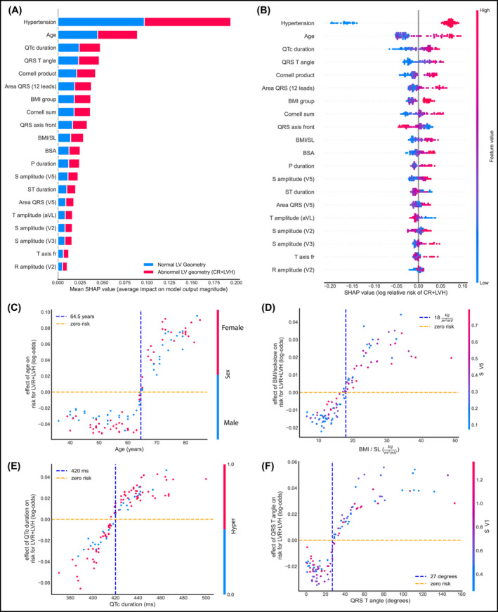
Global and local importance for the 20 most important features in the RF binary classifier for detecting CR+LVH, and feature interactions for four of them. All plots are on the test set. (A) Bar chart of mean feature importance for the classification. (B) SHAP summary plot showing the effect of each feature on individual patients. (C) Effect of Age on detecting CR+LVH. (D) Effect of the BMI/SL on detecting CR+LVH with a visible cutoff of around 18 kg/m²mV. (E) Effect of QRS‐T angle on the same risk. Risk appears higher after a value of 27 degrees (F) Effect of QTc duration on the same risk, with a visible cutoff point at 420 ms BMI, body mass index; BSA, body surface area; CR, concentric remodeling; ECG, electrocardiogram; LVH, left ventricular hypertrophy; NG, normal geometry; RF, random forest; SHAP, (SHapley Additive exPlanations)

3.3. Binary classification for classes NG+CR vs. LVH

Concentrating on the LVH class, we trained the RF to classify NG+CR vs. LVH. We achieved an accuracy of 88%, specificity 97%, sensitivity 44%, AUC/ROC 0.87, and AUC/PR 0.67 for a decision threshold of 0.5. Due to imbalance in the data set (ratio of NG+CR to LVH was 5/1), we performed oversampling for imbalance correction using Random Over Sampler. ³⁰ When we adjusted the threshold to 0.4, our results were accuracy of 89%, specificity 93%, sensitivity 67%, AUC/ROC 0.89, and AUC/PR 0.5. We chose the value 0.4 for the new threshold by inspecting the intersection point of the precision‐recall plot.

3.4. Multiclassification for classes NG vs. CR vs. LVH

When trained to classify patients into three classes, NG, CR, and LVH, our model achieved an accuracy was 74%, precision 65%, and sensitivity 88% for the CR category. Distinguishing the 3 categories enables us to gain insight on the features that contribute to an individual being classified in the CR category (Figure 5). From Figure 5D, we observe that individuals with hypertension combined with high QTc duration seem to have an increased risk of abnormal LVG.

FIGURE 5.

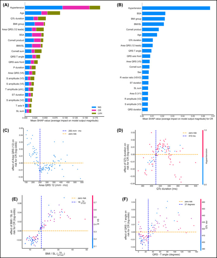
Global and local importance for 20 most important features in the RF 3‐class multiclassifier, detecting NG vs. CR vs. LVH, and feature interactions for four of them. All plots are on the test set. (A) Bar chart of mean global feature importance for distinguishing among the 3 classes. Colors indicate the importance of each feature to each category, with NG depicted by blue, CR by magenta, and LVH by green. (B) SHAP summary plot showing the effect of each feature on detecting specifically CR. (C) Effect of the area under the QRS interval summed over all 12 leads. (D) Effect of QTc duration on the same risk, with a visible cutoff point of 410 ms (E) Effect of the BMI/SL on detecting CR with a visible cutoff around 17 kg/m²mV. (F) Effect of QRS‐T angle on the risk of having CR. BMI, body mass index; BSA, body surface area; CR, concentric remodeling; ECG, electrocardiogram; LVH, left ventricular hypertrophy; NG, normal geometry; RF, random forest; SHAP, (SHapley Additive exPlanations)

3.5. Selected model

We selected the RF as our ML method, after trying other relevant approaches, such as a Boosting algorithm and a Support Vector Classifier (SVC). Specifically, Catboost ³¹ obtained an accuracy of 83%, while the SVC from the scikit‐learn package produced a mean accuracy of 83% and an AUC(ROC) value of 0.80, both models on the test set for NG vs. CR_LVH. RF was the best performing model for our dataset and also provided interpretability through the SHAP tools.

4. DISCUSSION

To our knowledge, this study is the first to demonstrate the promising potential of ML modeling for the efficient and cost‐effective diagnostic screening of abnormal LVG and cardiac remodeling through ECG. We found specific clinical and ECG features that can predict early pathological LVG changes in patients without established CVD. We also identified the population that will benefit from a detailed echocardiographic evaluation. We used not only the traditional ECG criteria for LVH, but also novel ECG markers that increased the accuracy of our ML model. Our findings are especially significant, since the majority of study participants had LV remodeling at very early stages without LVH, a situation that until now was not detectable by ECG but required imaging methods.

The detection of hypertension‐mediated organ damage, such as abnormal LVG, is a useful approach toward risk stratification of a hypertensive population. ¹⁵ The evaluation of cardiac structure and function is encouraged since it might influence treatment decisions. ¹⁵ Transthoracic echocardiography has received a strong indication for the initial evaluation of suspected hypertensive heart disease. Abnormal LVG is the early marker of LV remodeling that precedes hypertrophy and is frequently associated with LV diastolic dysfunction. ¹⁷ In hypertensive patients, the type of LVG and LV remodeling (CR, eccentric, and concentric LVH) is predictive of the incidence of cardiovascular (CV) events. ¹⁵ $\mathrm{CR}$ not only precedes LVH, but also most other cardiac dysfunctions, while it progresses asymptomatically. The early detection of abnormal LVG can result in timely identification of subclinical hypertension‐mediated organ damage and may help clinical decision and follow‐up.

ML classifiers, specifically RFs, trained on clinical information from the ECG (one of the most common non‐invasive diagnostic techniques) are capable of identifying patients with either LVH or LV remodeling at initial stages, versus normal individuals. Ensemble methods outperform any single base learner, such as Classification and Regression Decision Trees (CART). ²² For complex datasets, such as the one we have, linear‐based algorithms (eg, Logistic Regression) may not be sufficient in segmenting the class labels, leading to poor accuracies. More sophisticated algorithms, such as random forests, which can learn a non‐linear decision boundary, are more effective and can achieve higher accuracy scores.

Our findings show that age plays an important role in the risk of someone having CR or LVH, with a cutoff around 64.5 years of age. The risk appears higher for men younger than 64.5 years, while after that age, the risk seems higher for women. We also introduce the quotient of BMI and the BMI/SL because we hypothesize that body mass affects the amplitude of the R and S waves, as the electrical currents cover different distances. Indeed, our results indicate that BMI/SL seems to differentiate for the CR class. Hypertension, age, and BMI were most significant, as expected; the area under the QRS complex summed over all 12 leads, the Planar Frontal QRS‐T angle, and QTc duration, among others, were important in predicting risk.

There are limited studies in the literature that attempt to predict cardiac structural or functional abnormalities with ECG data interpreted through ML algorithms. ³² , ³³ , ³⁴ Previous work has focused only on patients who have already shown LVH. ³² , ³³ , ³⁴ , ³⁵ There are no data for patients in earlier stages of cardiac geometry change prior to hypertrophy. The present prospective ML study also differs from previous ones in that it involves patients who were very carefully selected, thereby excluding those with CVD. ³² , ³³ This may explain the fact that in our study, analysis of patients with LVH achieved a higher AUC in comparison with recently published work, ³² despite the fact that the number of our patients is smaller. ML is susceptible to major errors in interpretation and generalizability. The fact that participants in our study did not have CVD is a major strength, since in effect it eliminates other clinical parameters that could mislead our model. In this way, we improve the quality of input data and avoid various pitfalls that could arise due to the large diversity of pathological conditions that formed the basis for the training process.

The population of hypertensives in our study consists of patients with a relatively good profile in terms of clinical and echocardiographic characteristics. This is probably due to the fact that the vast majority of these patients were from the Hypertension Excellence Center of our department that provides a high level of inpatient and outpatient care. This further enhances the value of our results and indicates that the ECG contains a large amount of information directly associated with the underlying cardiac physiology independently of a patient's clinical status.

We have shown that a quantitative assessment of abnormal LVG can be performed by using easily obtained clinical data and ECG features. ECGs are more easily obtainable and cost‐effective than echocardiography or cardiac magnetic resonance imaging; for those reasons, they are more common in current clinical practice. Deep learning could potentially detect patients with hypertension‐mediated organ damage at an early stage, and with simple and widely used clinical tools. Digital methodologies open up new opportunities in health care quality, with the potential to advance personalized medicine at a lower cost. We showed that from basic clinical data and the use of the ECG, we can distinguish high‐risk patients such as the ones beginning to show CR; these are the ones requiring further evaluation, closer follow‐up and more detailed cardiovascular imaging. This initial evaluation can be performed in primary care facilities, or even out of office. Our model contributes to the development of human‐centered and autonomous technologies and can optimize patient management and treatment. This has become crucially important in recent times, due to the unprecedented demands on health care systems worldwide that the recent pandemic outbreak has imposed.

4.1. Limitations

The number of patients we have included is not large since this is a single‐center study over a specific time period. Nonetheless, our results are clear, especially due to the fact that our patient population is carefully chosen not to have CVD that could influence ECG features.

The RWT is not always reflective of true LVG in patients with asymmetric hypertrophy. On the other hand, it is the most widely used index for this purpose in routine clinical practice for hypertensive patients. ¹⁵ , ¹⁷ More studies are needed to test the applicability and transferability of our patients to other patients’ cohorts. Finally, we did not employ an external validation cohort, since this is a single‐center study, although 20% of our patients constitute validation (test) set. We currently plan to increase population size, as well as to obtain external validation. We cannot rule out the possibility that medications taken by some patients may change some of their ECG features. However, the analysis of this effect was beyond the scope of this study.

Finally, this model includes characteristics of QRS and QT from the ECG, so it cannot be easily applied in the presence of QRS or QT abnormalities.

5. CONCLUSION

In this study, we developed novel ML algorithms that are effective in the detection of patients with abnormal LVG even at very early stages, before the progression to LVH. Hypertension, age, BMI over the Sokolow‐Lyon voltage, QRS‐T angle, and QTc duration were some of the most important features used for this purpose. Our method offers an innovative strategy to improve health care management and personalized care at lower cost, especially in patients at risk for CVD, such as the hypertensive population. Further studies are required to determine whether our criteria can be broadly applied to other populations. Although there are still challenges in ML‐based applications to cardiology, research should be expanded since ML models can efficiently identify actionable insights into disease processes.

CONFLICT OF INTEREST

Professor Vardas has to report personal fees from MENARINI INTERNATIONAL, DEAN MEDICUS, SERVIER, EUROPEAN SOCIETY OF CARDIOLOGY, HYGEIA HOSPITALS GROUPS LTD, BAEYR. The other authors have nothing to declare. We also thank Kate Struth for language editing of the manuscript.

AUTHOR CONTRIBUTIONS

Eleni Angelaki, Maria Marketou, Georgios Barmparis, and Giorgos Tsironis involved in conceptualization. Eleni Angelaki, Maria Marketou, Georgios Barmparis, Alexandros Patrianakos, Panos Vardas, Fragiskos Parthenakis, and Giorgos Tsironis involved in validation. Eleni Angelaki, Georgios Barmparis, and Giorgos Tsironis involved in the analysis. Maria Marketou, and Alexandros Patrianakos involved in the collection of data. Eleni Angelaki, Maria Marketou, Georgios Barmparis, Alexandros Patrianakos, Fragiskos Parthenakis, and Giorgos Tsironis involved in data curation. Eleni Angelakia and Maria Marketou involved in writing—original draft preparation and project administration. Eleni Angelakia, Maria Marketou, Panos Vardas, and Giorgos Tsironis involved in writing—review and editing. Fragiskos Parthenakis and Giorgos Tsironis involved in supervision. All authors have read and agreed to the published version of the manuscript.

Angelaki E, Marketou ME, Barmparis GD, et al. Detection of abnormal left ventricular geometry in patients without cardiovascular disease through machine learning: An ECG‐based approach. J Clin Hypertens. 2021;23:935–945. 10.1111/jch.14200

REFERENCES

- 1. Haque A, Milstein A, Fei‐Fei L. Illuminating the dark spaces of healthcare with ambient intelligence. Nature. 2020;585:193‐202. [DOI] [PubMed] [Google Scholar]
- 2. Siontis KC, Yao X, Pirruccello JP, Philippakis AA, Noseworthy PA. How will machine learning inform the clinical care of atrial fibrillation? Circ Res. 2020;127:155‐169. [DOI] [PubMed] [Google Scholar]
- 3. Seetharam K, Raina S, Sengupta PP. The role of artificial intelligence in echocardiography. Curr Cardiol Rep. 2020;22(9):99. [DOI] [PubMed] [Google Scholar]
- 4. Lanzer JD, Leuschner F, Kramann R, Levinson RT, Saez‐Rodriguez J. Big data approaches in heart failure research. Curr Heart Fail Rep. 2020;17:213‐224. [DOI] [PMC free article] [PubMed] [Google Scholar]
- 5. Gilbert K, Mauger C, Young AA, Suinesiaputra A. Artificial intelligence in cardiac imaging with statistical atlases of cardiac anatomy. Front Cardiovasc Med. 2020;7:102. [DOI] [PMC free article] [PubMed] [Google Scholar]
- 6. Ganau A, Devereux RB, Roman MJ, et al. Patterns of left ventricular hypertrophy and geometric remodeling in essential hypertension. J Am Coll Cardiol. 1992;19:1550‐1558. [DOI] [PubMed] [Google Scholar]
- 7. Dweck MR, Joshi S, Murigu T, et al. Left ventricular remodeling and hypertrophy in patients with aortic stenosis: insights from cardiovascular magnetic resonance. J Cardiovasc Magn Reson. 2012;14:50. [DOI] [PMC free article] [PubMed] [Google Scholar]
- 8. Krumholz HM, Larson M, Levy D. Prognosis of left ventricular geometric patterns in the framingham heart study. J Am Coll Cardiol. 1995;25:879‐884. [DOI] [PubMed] [Google Scholar]
- 9. Devereux RB, Wachtell K, Gerdts E, et al. Prognostic significance of left ventricular mass change during treatment of hypertension. JAMA. 2004;292:2350‐2356. [DOI] [PubMed] [Google Scholar]
- 10. de Simone G, Izzo R, Chinali M, et al. Does information on systolic and diastolic function improve prediction of a cardiovascular event by left ventricular hypertrophy in arterial hypertension? Hypertension. 2015;56:99‐104. [DOI] [PubMed] [Google Scholar]
- 11. de Simone G, Kitzman DW, Chinali M, et al. Left ventricular concentric geometry is associated with impaired relaxation in hypertension: the HyperGEN study. Eur Heart J. 2005;26:1039‐1045. [DOI] [PubMed] [Google Scholar]
- 12. Park CS, Park JB, Kim Y, et al. Left ventricular geometry determines prognosis and reverse J‐shaped relation between blood pressure and mortality in ischemic stroke patients. JACC Cardiovasc Imaging. 2018;11:373‐382. [DOI] [PubMed] [Google Scholar]
- 13. Bressman M, Mazori AY, Shulman E, et al. Determination of sensitivity and specificity of electrocardiography for left ventricular hypertrophy in a large, diverse patient population. Am J Med. 2020;133:e495‐e500. [DOI] [PubMed] [Google Scholar]
- 14. Levy D, Labib SB, Anderson KM, et al. Determinants of sensitivity and specificity of electrocardiographic criteria for left ventricular hypertrophy. Circulation. 1990;81:815‐820. [DOI] [PubMed] [Google Scholar]
- 15. Williams B, Mancia G, Spiering W, et al. Practice Guidelines for the management of arterial hypertension of the European Society of Hypertension and the European Society of Cardiology: ESH/ESC Task Force for the Management of Arterial Hypertension. J Hypertens. 2018;2018(36):2284‐2309. [DOI] [PubMed] [Google Scholar]
- 16. Whelton PK, Carey RM, Aronow WS, et al. 2017 ACC/AHA/AAPA/ABC/ACPM/AGS/APhA/ASH/ASPC/NMA/PCNA Guideline for the prevention, detection, evaluation, and management of high blood pressure in adults: a report of the American College of Cardiology/American Heart Association task force on clinical practice guidelines. J Am Coll Cardiol. 2018;71:e127‐e248. [DOI] [PubMed] [Google Scholar]
- 17. Marwick TH, Gillebert TC, Aurigemma G, et al. Recommendations on the use of echocardiography in adult hypertension: a report from the European Association of Cardiovascular Imaging (EACVI) and the American Society of Echocardiography (ASE). J Am Soc Echocardiogr. 2015;28:727‐754. [DOI] [PubMed] [Google Scholar]
- 18. Van Rossum G, Drake FL. Python 3 reference manual. Scotts Valley, CA: CreateSpace; 2009. [Google Scholar]
- 19. Macfarlane PW. The frontal plane QRS‐T angle. Europace. 2012;14:773‐775. [DOI] [PubMed] [Google Scholar]
- 20. Neofotistos G, Mattheakis M, Barmparis GD, Hizanidis J, Tsironis GP, Kaxiras E. Machine learning with observers predicts complex spatiotemporal behaviour. Frontiers in Physics. 2019;7:24. [Google Scholar]
- 21. Seifert S. Application of random forest‐based approaches to surface‐enhanced Raman scattering data. Sci Rep. 2020;10:5436. [DOI] [PMC free article] [PubMed] [Google Scholar]
- 22. Breiman L. Random forests. Mach Learn. 2001;45:5‐32. [Google Scholar]
- 23. Hastie T, Tibshirani R, Friedman J. Elements of statistical learning: data mining, inference, and prediction. New York, NY: SpringerLink (Online service); Springer; 2009. [Google Scholar]
- 24. Pedregosa F, Varoquaux G, Gramfort A, Michel V, Thirion B. Scikit‐learn: machine learning in python. J Mach Learn Res. 2011;12:2825‐2830. [Google Scholar]
- 25. Probst P, Boulesteix A. To tune or not to tune the number of trees in random forest? 2017.
- 26. Lundberg SM, Erion GG, Lee S‐I.Consistent individualized feature attribution for tree ensembles. 2018.
- 27. Lundberg SM, Lee S‐I. A unified approach to interpreting model predictions. In: Guyon I, Luxburg UV, Bengio S, Wallach H, Fergus R, Vishwanathan S, Garnett R, eds. Advances in neural information processing systems 30. Curran Associates: Inc; 2017:4765‐4774. [Google Scholar]
- 28. Lundberg SM, Erion GG, Lee S‐I.Explainable AI for trees: from local explanations to global understanding. 2019. [DOI] [PMC free article] [PubMed]
- 29. Lundberg SM, Nair B, Vavilala MS, et al. Explainable machine‐learning predictions for the prevention of hypoxaemia during surgery. Nat Biomed Eng. 2018;2:749‐760. [DOI] [PMC free article] [PubMed] [Google Scholar]
- 30. Lematre G, Nogueira F, Aridas CK. Imbalanced‐learn: a python toolbox to tackle the curse of imbalanced datasets in machine learning. J Mach Learn Res. 2017;18:1‐5. [Google Scholar]
- 31. Prokhorenkova L, Gulin A. Catboost: unbiased boosting with categorical features. 2017.
- 32. Kagiyama N, Piccirilli M, Yanamala N, et al. Machine learning assessment of left ventricular diastolic function based on electrocardiographic features. J Am Coll Cardiol. 2020;76:930‐941. [DOI] [PubMed] [Google Scholar]
- 33. Sabovčik F, Cauwenberghs N, Kouznetsov D, et al. Applying machine learning to detect early stages of cardiac remodelling and dysfunction. Eur Heart J Cardiovasc. Imaging. 2020:jeaa135. (Online ahead of print). [DOI] [PubMed] [Google Scholar]
- 34. Sparapani R, Dabbouseh NM, Gutterman D, et al. Detection of left ventricular hypertrophy using bayesian additive regression trees: the MESA (multi‐Ethnic study of atherosclerosis). J Am Heart Assoc. 2019;8:e009959. [DOI] [PMC free article] [PubMed] [Google Scholar]
- 35. Kwon JM, Jeon KH, Kim HM, et al. Comparing the performance of artificial intelligence and conventional diagnosis criteria for detecting left ventricular hypertrophy using electrocardiography. Europace. 2020;22:412‐419. [DOI] [PubMed] [Google Scholar]