DeepCNV: a deep learning approach for authenticating copy number variations

Abstract

Copy number variations (CNVs) are an important class of variations contributing to the pathogenesis of many disease phenotypes. Detecting CNVs from genomic data remains difficult, and the most currently applied methods suffer from an unacceptably high false positive rate. A common practice is to have human experts manually review original CNV calls for filtering false positives before further downstream analysis or experimental validation. Here, we propose DeepCNV, a deep learning-based tool, intended to replace human experts when validating CNV calls, focusing on the calls made by one of the most accurate CNV callers, PennCNV. The sophistication of the deep neural network algorithm is enriched with over 10 000 expert-scored samples that are split into training and testing sets. Variant confidence, especially for CNVs, is a main roadblock impeding the progress of linking CNVs with the disease. We show that DeepCNV adds to the confidence of the CNV calls with an optimal area under the receiver operating characteristic curve of 0.909, exceeding other machine learning methods. The superiority of DeepCNV was also benchmarked and confirmed using an experimental wet-lab validation dataset. We conclude that the improvement obtained by DeepCNV results in significantly fewer false positive results and failures to replicate the CNV association results.

Introduction

Copy number variation (CNV), a type of structural variations (SVs) of the human genome with possible association with complex diseases such as schizophrenia [1] and osteoporosis [2], has received much attention in the past [3–5]. Detection of CNVs has become routine in genetic studies and in cancer research of disease susceptibility [6]. Using next-generation sequencing (NGS) to profile whole genomes, whole exomes or targeted regions has been currently widely adopted. NGS has emerged as a technology with the capability to detect both SNVs and structural variants [7, 8] in a single assay. However, CNV analysis via NGS is not trivial. Reliable CNV calls from NGS data demand high-sequencing depth and uniformity of coverage across all target sites, which may not be achievable in a cost- and time-effective manner. Consequently, microarray-based detection, as a cost-effective technique, remains a commonly ordered clinical genetic test and is expected to remain as an important CNV detection strategy for years to come [9]. Microarray-based computational calling algorithms, such as PennCNV [10] and QuantiSNP [11], have been widely employed for detecting CNVs. Nonetheless, the quantity and quality of CNVs reported by these methods on different platforms exhibit substantial variance. In particular, it is not uncommon to witness unacceptably high false positive rates of CNV calls. Winchester et al. [12] conducted comprehensive experiments to compare a number of algorithms, including Birdsuite 1.5.5 [13], CNAT (Genome Console 3.0.2) [12], GADA (R 0.7–5) [14], PennCNV [10] and QuantiSNP [11]. Although PennCNV demonstrated the best performance in terms of prediction accuracy, only 49% of the detected events could be confirmed [12, 15]. The high false positive rate may be minimized by only reporting the overlapped events from multiple algorithms [3], but at the expense of low sensitivity.

Compared with other methods, PennCNV incorporates multiple sources of information, including total signal intensity and allelic intensity ratio at each SNP marker, the distance between neighboring SNPs, the allele frequency of SNPs and the pedigree information. It enables kilobase-resolution detection of small-scale CNVs, which are common in the human genome [16–18]. In contrast, the resolution of CNV detection in previous experimental studies [19–22] was limited to tens or hundreds of kilobases [10]. Therefore, PennCNV has become a popular tool for CNV calling for clinical samples. However, to overcome the issue of high false positive rate, it is often recommended to visually examine CNV calls to judge whether they are reliable or not. For example, human experts can visualize and examine the log R ratio (LRR) and B allele frequency (BAF) scatter plot images using the Illumina BeadStudio software or the Affymetrix genotyping console. This additional manual screening step is laborious. Human experts may also be subjective and exhibit certain variance, which is not desired in a clinical setting.

Deep learning algorithms, powered by the advances in computation and very large datasets, have begun to exceed human performance in visual tasks such as playing Atari games and strategic board games such as Go [23]. Recently, deep learning has been successfully applied to genetics and biomedical studies [24–28]. Of note is the transfer RNA (tRNA)-DL [26], a deep learning approach that we have developed to improve the tRNAscan-SE prediction results. tRNAscan-SE [29] is the leading tool for tRNA annotation and prediction, which has been widely used in the field. However, tRNAscan-SE can still output a significant number of false positives. We used the tRNA sequences as positive samples and the false positive predictions made by tRNAscan-SE as negative samples to train a deep learning model, tRNA-DL. The trained tRNA-DL can effectively recognize and reduce the false positive outputs from tRNAscan-SE [26].

The success of tRNA-DL motivated us to develop a deep learning approach to reduce false positive CNV calls. In this study, we propose DeepCNV, a deep learning-based tool, which is intended to replace laborious manual filtering, for example, human visual check, in order to reduce false positive CNV calls. Given that humans can do screening based on the morphology of a curve shown in the scatter plot images, we expect that a learning algorithm taking into account some features of the curves can also solve the same problem. Using a deep learning approach can avoid building a handcrafted algorithm. DeepCNV employs a novel blended deep neural network structure and is capable of exploiting both image plots (image data) and summary statistics (meta data) output from PennCNV. This tool revolutionizes the ability of CNV studies to efficiently and effectively prune raw CNV callsets into confident CNV sets of high accuracy. The sophistication of the deep neural network algorithm is enriched with over 10 000 expert-scored samples split into training and testing sets. We show that DeepCNV significantly outperforms other machine learning methods. The superiority of DeepCNV was also benchmarked and confirmed using an experimental validation dataset. The improvement made by DeepCNV leads to less false positives and failures to replicate associations that plague the CNV genome-wide association study community. Broadly, high confidence in variant sets will lead to a more accurate determination of pathogenic CNVs underlying the disease states.

Materials and methods

Experimental data

Human-labeled dataset

We profiled 341 unique and independent healthy human samples using SNP microarray genotyping (Illumina Omni 2.5). PennCNV was applied with default settings to make CNV calls. Collectively, we obtained 10 748 CNVs output from PennCNV.

Image data

To visually examine the CNV calls and judge whether they are true positives or not, we utilized the auxiliary visualization program (visualize_cnv.pl) provided by PennCNV to generate image files for the CNV calls, automatically. For each CNV call, it produces one LRR scatter plot image and one BAF scatter plot image. The plots cover a candidate CNV segment and its surrounding regions. The LRR plot draws a point for each SNP genotyped in the region (candidate CNV + its extended regions), with chromosome position as the X-coordinate and LRR as the Y-coordinate. The BAF plot covers the same region with a similar plot but uses BAF as the Y-coordinate. For both plots, we color the SNPs (points) in the candidate CNV in red and the SNPs in the surrounding region in blue. Scientist with expertise in CNV calling then labeled them as either false positive or true positive based on visualization. Figure 1 depicts the sample images. The images were used as input for DeepCNV. The pixels in the images range from 0 to 255. Following a standard image scaling operation, we normalized the pixel values by dividing each pixel by 255, so the new values ranged between 0 and 1 for use by DeepCNV.

Figure 1 .

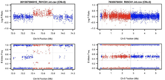
Two representative examples of the CNV image data. LRR scatter plot is on the top and BAF scatter plot is on the bottom. Both plots are drawn against the same SNP positions. Right panels show a false positive call made by PennCNV (a sample without CNV) in which the LRR dots concentrate around zero reference line and the BAF dots show three normal kinds of B Alleles, for example, AA, AB and BB. Left panels show a true positive call (a sample with CNV) in which the LRR dots colored red are above the zero reference line and BAF dots colored red show four kinds of B Alleles, for example, BBB, ABB, AAB and AAA.

Meta data

PennCNV also generates summary statistics for quality checking. The summary statistics consist of 13 features as shown in Table 1, which we reference as meta data. Z-score normalization was applied to each of the features so that they have a comparable range. Both DeepCNV and the competing machine learning methods use meta data as input.

Table 1.

Summary of the meta data

Index	Feature name	Data type	Data range	Description
1	Call rate	Float	[0.978, 0.999]	Simple SNP genotyping call rate
2	Length	Float	[31, 6 455 331]	The CNV length
3	CN	Integer	[0, 4]	The number of CN
4	Number of SNPs	Integer	[3, 5995]	The number of independent SNP markers
5	PennCNV Confidence	Float	[14.64, 13758.3]	The call confidence of PennCNV
6	Number of CNVs in Sample	Integer	[18, 911]	Inflated numbers of false positive CNV calls
7	LRR_mean	Float	[−0.035, 0.024]	The mean of LRR
8	LRR_SD	Float	[0.10, 0.27]	The SD of LRR
9	BAF_mean	Float	[0.498, 0.511]	The mean of BAF
10	BAF_SD	Float	[0.029, 0.057]	The SD of BAF
11	BAF_DRIFT	Float	[0.000, 0.003]	BAF drift
12	WF	Float	[−0.02, 0.031]	Waviness factor
13	GCWF	Float	[−0.006, 0,009]	The GC base content adjusted waviness factor

PennCNV log file meta data giving insight into the relative data quality of each sample to condition image review. WF: Waviness Factor; GCWF: Guanine Cytosine Waviness Factor.

Sample information

Out of the 10 748 CNV calls, 6858 of them were labeled as negative (false positive) samples. Generally, the larger the size of CNV, the easier to detect. Among the 10 748 CNVs, 2505 are small (0.1–5 kb), 3941 are medium (5–20 kb) and 4302 are large (>20 kb). For CNVs within these three size ranges, we kept the same positive/negative ratio, and we randomly split the data into the training (70%), validation (15%) and testing (15%) datasets as shown in Table 2. In addition, we also performed the 10-fold cross-validation for evaluation.

Table 2.

Summary of the human-labeled samples

CNV size	Training (70%)		Validation (15%)		Testing (15%)		Total
	POS	NEG	POS	NEG	POS	NEG
0–5 kb (Small)	746	1006	160	216	161	216	2505
5–20 kb (Medium)	1043	1715	224	367	224	368	3941
>20 kb (Large)	932	2079	200	445	200	446	4302
Subtotal	2721	4800	584	1028	585	1030	10 748
Total	7512		1612		1615		10 748

‘NEG’ and ‘POS’ represent the false positive and true positive samples from PennCNV, respectively.

Sequencing-derived CNV

We note that the utility of our method for reducing false positive calls is generalized and not limited to any particular CNV callers or genotyping platforms. To demonstrate this point, we collect a dataset for which CNV calls are made using several other CNV callers from whole genome sequencing (WGS) data. A recent study has constructed an integrated map of SV including CNV in 2504 human genomes [30]. The authors performed SV discovery and genotyping using an ensemble of nine different algorithms followed by several orthogonal experimental platforms for SV set assessment, refinement and characterization. We extracted the deletions and duplications >10 Kb in their release as true positives. We obtained the raw CNV call files from the supporting input call sets folder of the 1000 genomes FTP site. The CNVs that are filtered out and not in the final release are considered as false positives. As a result, we obtained a WGS CNV dataset of 12 509 positive and 4373 negative CNVs (>10 kb) for benchmarking our method. This dataset also suggests that the false positive rate is as much as 25% if no manual filtering and refinement are applied. For the sequencing data, we generate LRR and BAF in a comparable manner to that of the SNP array data calls [31].

Experimentally validated dataset

We experimentally validated 616 array-based CNV calls using qPCR. Of those, 520 samples were confirmed to be true positives, while 96 samples turned out to be false positives. qPCR was performed using TaqPath ProAmp Master Mix (ThermoFisher Scientific). Taqman assays targeting the desired regions were identified using the ThermoFisher Scientific website tools and were selected to be compatible with the hTERT reference Taqman assay. Genomic DNA, 10 ng, was included in each reaction, along with the indicated Taqman assay and the hTERT reference assay in a reaction volume of 10 ml. Each reaction was run in triplicate. For each assay, three controls were run along with subject samples: a no-template control (water alone) and commercial sources of male and female genomic DNA (Promega). PCR was performed on a Viia 7 Real-Time PCR system (ThermoFisher Scientific) using cycling conditions recommended for the TaqPath ProAmp master mix for copy number (CN) variant detection (standard cycling conditions: 95°C for 10 min to activate the enzyme, followed by 40 cycles of 95°C for 15 s and 60°C for 1 min). Data were exported to text file using the QuantStudio Real-Time PCR Software v1.2 (ThermoFisher Scientific) and imported to the Copy Caller v2.1 for analysis (ThermoFisher Scientific). Analysis of each Taqman assay was performed in the Copy Caller using the commercial male DNA as the calibrator sample. Normal CN of the commercial female DNA was confirmed as a control as was the failure of amplification in the no-template control sample.

DeepCNV framework

To fully explore the available information, we constructed a blended deep neural network with two branches, a deep convolutional neural network [32] (CNN) and a deep fully connected neural network (DNN), to simultaneously model the image data and meta data. We present the network architecture in Figure 2. CNN is one of the most popular deep learning architectures and has demonstrated state-of-the-art performance for visual applications [32–35]. The CNN part of our DeepCNV model is composed of a stack of convolutional layers, where we use filters with a receptive field of 3 3. The convolution stride is fixed to 1 pixel. All convolutional layers are equipped with LeakyReLU activations [36]. Max-pooling is performed over a window, with stride 2. Mathematically, each convolutional layer computes

where is the input image or the output from the previous layer, is the index of convolutional filter kernel and is the index of output position. Filter is the weight matrix, with and being the width and length of the filter, and being the input channel dimension. Specifically, is for all convolutional layers. LeakyReLU [36] represents the leaky rectified linear unit, which is defined as follows:

where is a parameter. If is 0, LeakyReLU is equivalent to ReLU [37]. The parameter of LeakyReLU is tuned on training data and is set to be 0.001 for all activation layers. In addition, we apply the dropout regularization [38], with a dropout probability of 0.4, to prevent overfitting. As shown in Figure 2, there are five convolutional layers with a number of filters (32, 64, 64, 128 and 128). The input to the CNN branch is a fixed-size of RGB image.

Figure 2 .

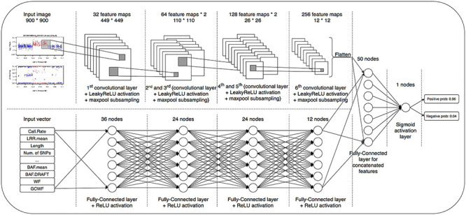
The architecture of DeepCNV model. The upper part is the CNN for modeling the image data. The lower part is the DNN for modeling the meta data.

The second branch is a pure fully connected neural network to learn how the meta data contribute to the final decision. This network accepts a numerical input vector with a length equal to 13 and is then followed by four layers with (36, 24, 24 and 12) neurons, respectively. The two branches are flattened, concatenated and fed into a dense layer with 50 neurons, followed by the final sigmoid activation node to generate the score for classifying false positive from the true positive samples. The optimizer is RMSprop [39] with a learning rate of .

We show how a CNV image looks like in the eye of DeepCNV model when it ‘annotates’ CNV calls. To this end, we employ a technique called Grad-CAM [40] to visualize the regions that are important for CNV prediction. The class-specific gradient information flowing into the final convolutional layer of the CNN has been used to generate a coarse localization map of the important regions of the input image. We show the pipeline in Figure 3. In order to obtain the class-discriminative localization map, we first compute the gradient of the score for class , with respect to feature maps of a convolutional layer. The gradients flowing back are averaged to obtain the neuron importance weight, , as follows:

where refers to the activation at location of the feature map and . The weight represents the importance of feature map for a target class . We perform a weighted combination of forward activation maps and apply an additional ReLU [37] operation, as we are interested in the features that have positive impacts on the class of interest. As shown in Figure 3, we resize the importance score of each pixel to and highlight the regions that are most valuable to the current prediction.

Figure 3 .

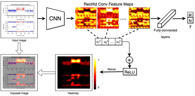
The Grad-CAM pipeline. The Grad-CAM pipeline detects important regions of the image data.

Results

We trained DeepCNV using the training set, tuned its hyperparameters using the validation set and evaluated it using the test set. DeepCNV consists of two main branches, CNN for image data and DNN for meta data. To demonstrate the contribution of each branch and the utility of the image data and meta data, we also evaluated its two reduced versions, CNN and DNN. The CNN only keeps the CNN branch and takes only image data as input, while DNN employs only the DNN branch with only meta data as input. We compared DeepCNV with DNN, CNN and other popular machine learning methods, including support vector machine (SVM) [41], random forest (RF) [42] and logistic regression (LR). SVM, RF and LR were implemented using scikit-learn library with recommended hyperparameters [43]. Note that SVM, RF, LR and DNN use meta data as the input, while the input for CNN are the image data.

Results on human-labeled dataset

In Figure 4, we show the prediction performance of the methods in terms of the area under the receiver operating characteristic (ROC) curve (AUC) on the testing dataset (Supplementary Table S1, available online at https://academic.oup.com/bib, shows the numerical AUC score of each classifier). A few remarks about the prediction results are noteworthy. Firstly, DeepCNV achieved the best prediction performance across different length of CNVs with an overall AUC of 0.909, followed by CNN and then DNN. Secondly, DeepCNV (meta data + image data) outperformed both CNN (using image data only) and DNN (using meta data only), with the performance of CNN being closer to the optimal. It suggests that both kinds of data are useful: each provide some complementary information that the other one does not have, while the image data may be more informative than the meta data. Thirdly, the smaller the CNV, the harder the prediction. DeepCNV brings the largest improvement for small CNVs (<5 kb), which are the most challenging cases. Fourthly, for the large CNVs (>20 Kb), the AUC of DeepCNV reaches 0.958, which is promising and is keeping with the clinical performance standards. Collectively, our results demonstrate that DeepCNV performs best among competing machine learning algorithms in terms of deliverables from learning from the human-labeled CNV samples. The classifiers show similar performance under 10-fold cross-validation (Supplementary Table S2 available online at https://academic.oup.com/bib).

Figure 4 .

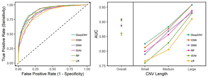
Prediction performance on the human-labeled dataset. The left panel presents the ROC curves. The right panel shows the overall AUC values and the AUC values stratified by the CNV sizes.

Not only can DeepCNV provide a binary decision (CNV or not), but it can also produce a probability of an event being a CNV. Based on the predicted CNV probability from low to high (0–1), we divide the testing samples into 10 tiers and summarize the total number of samples in each tier as shown in Figure 5. We further stratify the samples based on their CNs estimated by PennCNV, and we highlight true positive portions in red. We can see that for all scenarios (CN = 0, 1 and 3), the higher the predicted probability of DeepCNV, the more likely a CNV call is a true positive event. Therefore, the predicted probability can be used for effectively prioritizing candidate calls. For example, a more stringent cutoff may be applied in the clinical setting if we want to achieve a high positive predictive value (PPV). It is not supervising that recognizing homozygous deletion (CN = 0) is the easiest case: when the probability is higher than 0.5, DeepCNV achieves a 100% consistency with human labeling. When there is one copy deviation, it is interesting to see hemizygous deletion (CN = 1) is harder to predict than hemizygous duplication (CN = 3). For hemizygous deletion, the predicted probabilities spread over from 0 to 1. Quite a few cases center around a probability of 0.5 from which we observe the largest disagreement between DeepCNV and human experts. For hemizygous duplication, in contrast, DeepCNV is more confident with its prediction, with most samples having a probability of either less than 0.1 or larger than 0.9, which is agreeing well with the human judgment. For homozygous duplication (CN = 4), we have too few samples (less than 10) to draw any conclusion.

Figure 5 .

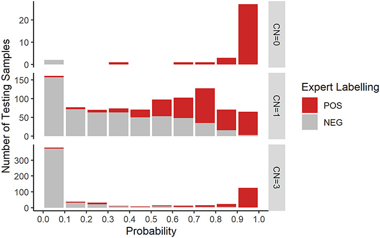
Consistency between DeepCNV and human expert labeling in different CN scenarios. The CN refers to the actual integer CN estimates calculated by PennCNV [10], and the normal CN is 2. For autosome, CN = 0 or 1 means there is a deletion and CN ≥ 3 means there is a duplication [10].

The superior performance of DeepCNV is attributed to its deep network structure, which uses several hidden layers to learn a high-level representation of CNV images hierarchically. To elucidate the power of this hierarchical representation and learning, we visualized the positive and negative samples using t-SNE [44] based on the last hidden layer representations in the CNN (Figure 6). We can see that the features become discriminative after several layers of transformation, culminating with a clear separation in the output layer.

Figure 6 .

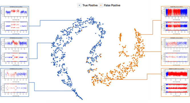
t-SNE visualization of the last hidden layer representations in the CNN for two image classes. Here, we show the CNN’s internal representation of four important disease classes by applying t-SNE, a method for visualizing high-dimensional data, to the last hidden layer representation in the CNN. Colored point clouds represent the different image categories, showing how the algorithm clusters the images. Insets show images corresponding to various points.

Comparison with other existing deep learning architectures

To quantify the contribution of the proposed network structures, we compared DeepCNV with two popular existing deep learning architectures, VGG19 [45] and ResNet34 [46]. We replaced the CNN structure in DeepCNV with the backbone of VGG19 and ResNet34, respectively. As shown in Supplementary Table S3 available online at https://academic.oup.com/bib, DeepCNV compares favorably to that of VGG19, and both outperform ResNet34. Compared to our network structures, ResNet and VGG19 have more convolutional layers, which may be more suitable for capturing richer textures. Here, the CNV images only contain isolated points, and sophisticated architectures may not necessarily help.

Comparison with other existing feature extraction methods

Based on the previous results, it is clear that images are useful but not ready for use by the classical machine learning methods. To overcome this problem, we consider two well-known feature extraction methods, SIFT [47] and autoencoder. The autoencoder uses six Conv2D and MaxPooling layers as encoder and six Conv2DTranspose layers as decoder. We apply SIFT and autoencoder to extract features from the images, concatenate the extracted image features with meta data and use them as input of LR, RF and SVM. Their performances under 10-fold cross-validation are shown in Supplementary Table S4 available online at https://academic.oup.com/bib. We find that that using the features extracted from images can bring improvement over the corresponding approaches using only meta data as the input in most cases, except RF is better than RF with the SIFT-extracted features. Despite the fact that these competing methods are improved with the extracted features, DeepCNV still outperforms them. These results indicate that separating feature engineering (feature extraction) from model fitting may not be an optimal strategy.

Results on WGS CNVs

The 12 509 positive images and 4373 negative images come from 2465 WGS samples, among which 523 samples contain both positive and negative images, 1938 samples only contain positive images and 4 samples only contain negative images. The imbalanced ratio between the positive and negative images is around 2.86:1. We randomly split those images into the training, validation and testing sets with a sample size ratio of around 3:1:1 and keep the imbalanced positive/negative ratio in each fold almost the same. We split the images by samples such that all the images of the same sample are assigned to only one set, namely, either training, validation or testing. DeepCNV yielded an almost perfect AUC of 0.9991 on the testing set (2500 positive and 873 negative images) with an AUC of 0.9991. This almost perfect prediction suggests that DeepCNV could replace the laborious manual filtering and refinement used in the original study [30] for reducing false positives.

Results on experimentally validated dataset

We collected an experimentally validated dataset to benchmark our method in comparison with the human experts. DeepCNV model trained on the manually labeled dataset was applied to test on these 616 experimentally validated samples. A human expert was also tested on the same dataset simultaneously. The human expert achieved a PPV of 0.924, which was a bit higher than the PPV of 0.893 for DeepCNV. However, DeepCNV obtained a sensitivity of 0.833, which is much higher than the sensitivity of 0.484 for the human expert. Overall, the DeepCNV yielded a F1 score of 0.862, which is much larger than the F1 score of 0.635 achieved by the human expert. This testing set has a high true positive rate (520/616 = 84%). The human expert tends to be stringent and rejects a substantial number of cases based on his prior training and experience. Consequently, during the testing procedure, the human expert may unconsciously reject more cases to meet his prior expectation, which probably explains the inferior performance of the human being in this testing experiment.

How a CNV image looks to DeepCNV

We show how a CNV image looks like in the eye of DeepCNV when it ‘annotates’ CNV calls. An example of feature importance heatmap calculated by Grad-CAM is shown in Figure 7. With Grad-CAM technique, we know that DeepCNV weighs the deviations from the reference line when deciding. This artificial intelligence of DeepCNV is similar to the logic of human expert during the decision-making process. The important heatmap yields insights into the relative importance of LRR and BAF in the predicted CNV region as well as the flanking region for various CN states. In contrast, we expect sample ID and axis labels are irrelevant to the CNV status, and interestingly, those parts have no intensity in the heatmap. In other words, DeepCNV ignores those parts when making its judgment calls. Thus, the trained DeepCNV model values the same part of image data as the human expert when it authenticates the CNV calls.

Figure 7 .

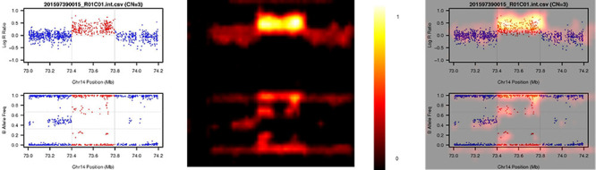
An example of feature importance heatmap from Grad-CAM pipeline. The left panel is the original image; the middle panel is the heatmap (the yellower, the more important) and the right panel combines the original image and the heatmap to show the highlighted part of original image.

Conclusion and Discussion

Standard approaches for identifying CNVs rely on the predictions from the CNV tools (such as PennCNV) followed by laborious and heuristic filtering. However, manually differentiating the false positives from the true positives becomes less affordable when the sample size is large. In addition, manual filtering may be subjective to and could introduce bias, while workflow rigidity and objectives are desired in clinical settings. DeepCNV is designed to fill this gap and serve the purpose of automating the filtering process in a transparent and objective way. The hierarchical structure of DeepCNV compresses the original data from intractable large dimension into a feasible and informative representation to increase the distinguishability.

Given the low dimensionality of the data in the images, a 1D convolution-based network could be considered to take the raw data instead of the image as the input. It is noted that different candidate CNVs have different lengths, and their data points have different densities. We need to truncate a long CNV or pad a short CNV with 0s to be of the same length in order to apply 1D convolution-based networks. However, the lengths of CNVs and the densities of their data points have a wide range so this strategy may not work optimally. Recurrent neural networks (RNN) may be an alternative for handling the varied lengths but may not be good at characterizing the data points profiled at the various densities. Another issue is to integrate two data vectors of LRR and BAF. Our solution of converting the data vectors into images of the same size helps to avoid these problems and allows us to exploit the power of CNNs.

DeepCNV can be coupled with any CNV callers that are plagued by false positives. We can similarly generate LRR and BAF images and relevant meta data for candidate CNV calls made by any CNV tools. DeepCNV then can be trained using the same pipeline. Nevertheless, it may be more desired if the deep learning-based method can be an end-to-end procedure which eliminates the dependence on the CNV callers to generate raw CNV calls. Thus, we aim to recognize CNVs directly from the raw data using deep learning. Namely, given the genomic data of a sample, we hope to detect the CNVs in it, if any. We may formulate it as a segmentation problem in image analysis. But it is more challenging in that the object of interest (CNV) can be much similar as the background and sometimes it is small, which makes the task like finding a needle in a haystack. To alleviate the challenge, we may provide and utilize true CNVs that have been annotated and validated. Then it becomes a semi-supervised learning problem. But this is not a conventional semi-supervised learning problem and is more challenging because the labeled CNVs have different sizes as the unlabeled long input sequences. Previous works show that deep learning can deal with complex and long bioinformatic sequences [48–50]. With those recent advancements, we may develop an end-to-end solution. We leave these explorations to future work. Altogether, we can foresee that the detection routine would become much more intelligent in the near future.

Key Points

• DeepCNV fills a critical gap of CNV authentication from any CNV detection algorithm.

• Curation of CNVs is typically done by a laborious manual review which is inconsistent, which has been successfully replaced here by machine learning.

• Here, we present a model trained by an extensive manual visual review with a tunable probability of negative versus positive prediction to achieve >90% sensitivity and specificity.

Joseph T. Glessner, PhD, is the Technical Director at the Genetics Core Facility in the Center for Applied Genomics at the Children’s Hospital of Philadelphia. Dr Glessner’s current research focuses on childhood neuropsychiatric and neurodevelopmental disorders along with the genetic architecture associated with them, including single nucleotide polymorphisms, single nucleotide variations and copy number variations ascertained by genomic technologies.

Xiurui Hou, PhD, is a recent graduate of the Department of Computer Science at the New Jersey Institute of Technology.

Cheng Zhong is a graduate student in the Department of Computer Science at the New Jersey Institute of Technology.

Jie Zhang, PhD, is a senior machine learning research scientist at Adobe Inc.

Munir Khan is a bioinformatics analyst at the Center for Applied Genomics at the Children’s Hospital of Philadelphia.

Fabian Brand is a postdoctoral researcher at the University of Bonn in Germany.

Peter Krawitz, PhD, is a Professor at the University of Bonn in Germany.

Patrick M. A. Sleiman, PhD, is the Co-Director at the Center for Applied Genomics at the University of Pennsylvania School of Medicine.

Hakon Hakonarson, MD, PhD, is an Endowed Chair and a Professor of pediatrics and a Director at the Center for Applied Genomics at the University of Pennsylvania School of Medicine.

Zhi Wei, PhD, is a Professor of computer science in the Department of Computer Science at the New Jersey Institute of Technology.

Data availability

The software is implemented in python and can be freely downloaded from the GitHub repository (https://github.com/CAG-CNV/DeepCNV). Data have been deposited in NCBI’s database of Genotypes and Phenotypes (dbGaP) through study accession numbers: phs000490.v1.p1, phs000607.v3.p2, phs000371.v1.p1, phs000490.v1.p1, phs001194.v2.p2, phs001194.v2.p2.c1, phs001661 and phs000233.

Funding

The Children’s Hospital of Philadelphia Endowed Chair in Genomic Research (NHGRI-sponsored eMERGE Network) (U01-HG006830 to Dr H.H.); the Children’s Hospital of Philadelphia (Institutional Development Fund to the Center for Applied Genomics); Extreme Science and Engineering Discovery Environment (XSEDE) (CIE170034) [supported by the National Science Foundation (grant no. ACI-1548562)].

References

- 1.Consortium IS. Rare chromosomal deletions and duplications increase risk of schizophrenia. Nature 2008;455:237. [DOI] [PMC free article] [PubMed] [Google Scholar]
- 2.Yang T-L, Chen X-D, Guo Y, et al. Genome-wide copy-number-variation study identified a susceptibility gene, UGT2B17, for osteoporosis. Am J Hum Genet 2008;83:663–74. [DOI] [PMC free article] [PubMed] [Google Scholar]
- 3.Pinto D, Darvishi K, Shi X, et al. Comprehensive assessment of array-based platforms and calling algorithms for detection of copy number variants. Nat Biotechnol 2011;29:512. [DOI] [PMC free article] [PubMed] [Google Scholar]
- 4.Curtis C, Lynch AG, Dunning MJ, et al. The pitfalls of platform comparison: DNA copy number array technologies assessed. BMC Genom 2009;10:588. [DOI] [PMC free article] [PubMed] [Google Scholar]
- 5.Hester SD, Reid L, Nowak N, et al. Comparison of comparative genomic hybridization technologies across microarray platforms. J Biomol Tech 2009;20:135. [PMC free article] [PubMed] [Google Scholar]
- 6.Cho E, Tchinda J, Freeman J, et al. Array-based comparative genomic hybridization and copy number variation in cancer research. Cytogenet Genome Res 2006;115:262–72. [DOI] [PubMed] [Google Scholar]
- 7.Carson AR, Feuk L, Mohammed M, et al. Strategies for the detection of copy number and other structural variants in the human genome. Hum Genomics 2006;2:403. [DOI] [PMC free article] [PubMed] [Google Scholar]
- 8.Pang AW, MacDonald JR, Pinto D, et al. Towards a comprehensive structural variation map of an individual human genome. Genome Biol 2010;11:R52. [DOI] [PMC free article] [PubMed] [Google Scholar]
- 9.Miller DT, Adam MP, Aradhya S, et al. Consensus statement: chromosomal microarray is a first-tier clinical diagnostic test for individuals with developmental disabilities or congenital anomalies. Am J Hum Genet 2010;86:749–64. [DOI] [PMC free article] [PubMed] [Google Scholar]
- 10.Wang K, Li M, Hadley D, et al. PennCNV: an integrated hidden Markov model designed for high-resolution copy number variation detection in whole-genome SNP genotyping data. Genome Res 2007;17:1665–74. [DOI] [PMC free article] [PubMed] [Google Scholar]
- 11.Colella S, Yau C, Taylor JM, et al. QuantiSNP: an Objective Bayes Hidden-Markov Model to detect and accurately map copy number variation using SNP genotyping data. Nucleic Acids Res 2007;35:2013–25. [DOI] [PMC free article] [PubMed] [Google Scholar]
- 12.Winchester L, Yau C, Ragoussis J. Comparing CNV detection methods for SNP arrays. Brief Funct Genomic Proteomic 2009;8:353–66. [DOI] [PubMed] [Google Scholar]
- 13.Korn JM, Kuruvilla FG, McCarroll SA, et al. Integrated genotype calling and association analysis of SNPs, common copy number polymorphisms and rare CNVs. Nat Genet 2008;40:1253. [DOI] [PMC free article] [PubMed] [Google Scholar]
- 14.Pique-Regi R, Monso-Varona J, Ortega A, et al. Sparse representation and Bayesian detection of genome copy number alterations from microarray data. Bioinformatics 2008;24:309–18. [DOI] [PMC free article] [PubMed] [Google Scholar]
- 15.Kidd JM, Cooper GM, Donahue WF, et al. Mapping and sequencing of structural variation from eight human genomes. Nature 2008;453:56. [DOI] [PMC free article] [PubMed] [Google Scholar]
- 16.Tuzun E, Sharp AJ, Bailey JA, et al. Fine-scale structural variation of the human genome. Nat Genet 2005;37:727. [DOI] [PubMed] [Google Scholar]
- 17.Conrad DF, Hurles ME. The population genetics of structural variation. Nat Genet 2007;39:S30. [DOI] [PMC free article] [PubMed] [Google Scholar]
- 18.Freeman JL, Perry GH, Feuk L, et al. Copy number variation: new insights in genome diversity. Genome Res 2006;16:949–61. [DOI] [PubMed] [Google Scholar]
- 19.Iafrate AJ, Feuk L, Rivera MN, et al. Detection of large-scale variation in the human genome. Nat Genet 2004;36:949. [DOI] [PubMed] [Google Scholar]
- 20.Ishkanian AS, Malloff CA, Watson SK, et al. A tiling resolution DNA microarray with complete coverage of the human genome. Nat Genet 2004;36:299. [DOI] [PubMed] [Google Scholar]
- 21.Scherer SW, Lee C, Birney E, et al. Challenges and standards in integrating surveys of structural variation. Nat Genet 2007;39:S7–15. [DOI] [PMC free article] [PubMed] [Google Scholar]
- 22.Wong KK, deLeeuw RJ, Dosanjh NS, et al. A comprehensive analysis of common copy-number variations in the human genome. Am J Hum Genet 2007;80:91–104. [DOI] [PMC free article] [PubMed] [Google Scholar]
- 23.Silver D, Schrittwieser J, Simonyan K, et al. Mastering the game of go without human knowledge. Nature 2017;550:354–9. [DOI] [PubMed] [Google Scholar]
- 24.Angermueller C, Pärnamaa T, Parts L, et al. Deep learning for computational biology. Mol Syst Biol 2016;12:878. [DOI] [PMC free article] [PubMed] [Google Scholar]
- 25.Gao X, Zhang J, Wei Z, et al. DeepPolyA: a convolutional neural network approach for polyadenylation site prediction. IEEE Access 2018;6:24340–9. [Google Scholar]
- 26.Gao X, Wei Z, Hakonarson H. tRNA-DL: a deep learning approach to improve tRNAscan-SE prediction results. Hum Hered 2018;83:163–72. [DOI] [PubMed] [Google Scholar]
- 27.Chang P, Grinband J, Weinberg B, et al. Deep-learning convolutional neural networks accurately classify genetic mutations in gliomas. Am J Neuroradiol 2018;39:1201–7. [DOI] [PMC free article] [PubMed] [Google Scholar]
- 28.Tian T, Wan J, Song Q, et al. Clustering single-cell RNA-seq data with a model-based deep learning approach. Nat Mach Intell 2019;1:191. [Google Scholar]
- 29.Lowe TM, Eddy SR. tRNAscan-SE: a program for improved detection of transfer RNA genes in genomic sequence. Nucleic Acids Res 1997;25:955–64. [DOI] [PMC free article] [PubMed] [Google Scholar]
- 30.Sudmant PH, Rausch T, Gardner EJ, et al. An integrated map of structural variation in 2,504 human genomes. Nature 2015;526:75–81. [DOI] [PMC free article] [PubMed] [Google Scholar]
- 31.Araujo Lima L, Wang K. PennCNV in whole-genome sequencing data. BMC Bioinform 2017;18:383. [DOI] [PMC free article] [PubMed] [Google Scholar]
- 32.LeCun Y, Bengio Y, Hinton G. Deep learning. Nature 2015;521:436. [DOI] [PubMed] [Google Scholar]
- 33.Krizhevsky A, Sutskever I, Hinton GE. Advances in neural information processing systems. Advances in Neural Information Processing Systems, 2012, 1097–105.
- 34.Szegedy C, Vanhoucke V, Ioffe S, et al. Rethinking the inception architecture for computer vision. Proceedings of the IEEE Conference on Computer Vision and Pattern Recognition, 2016, 2818–26.
- 35.Kim Y. Convolutional neural networks for sentence classification. In Proceedings of the 2014 Conference on Empirical Methods in Natural Language Processing, EMNLP 2014. [DOI] [PMC free article] [PubMed]
- 36.Maas AL, Hannun AY, Ng AY. Rectifier nonlinearities improve neural network acoustic models, in ICML Workshop on Deep Learning for Audio, Speech and Language Processing, 2013.
- 37.Nair V, Hinton GE. Rectified linear units improve restricted boltzmann machines. Proceedings of the 27th International Conference on Machine Learning (ICML-10), 2010, 807–14.
- 38.Srivastava N, Hinton G, Krizhevsky A, et al. Dropout: a simple way to prevent neural networks from overfitting. J Mach Learn Res 2014;15:1929–58. [Google Scholar]
- 39.Tieleman T, Hinton G. Lecture 6.5-rmsprop: Divide the gradient by a running average of its recent magnitude. COURSERA: Neural Networks for Machine Learning, 4, 2012.
- 40.Selvaraju RR, Cogswell M, Das A, et al. Grad-cam: Visual explanations from deep networks via gradient-based localization. Proceedings of the IEEE International Conference on Computer Vision, 2017, 618–26.
- 41.Suykens JA, Vandewalle J. Least squares support vector machine classifiers. Neural Proc Letters 1999;9:293–300. [Google Scholar]
- 42.Liaw A, Wiener M. Classification and regression by randomForest. R News 2002;2:18–22. [Google Scholar]
- 43.Pedregosa F, Varoquaux G, Gramfort A, et al. Scikit-learn: machine learning in python. J Mach Learn Res 2011;12:2825–30. [Google Scholar]
- 44.Maaten L, Hinton G. Visualizing data using t-SNE. J Mach Learn Res 2008;9:2579–605. [Google Scholar]
- 45.Simonyan K, Zisserman A. Very Deep Convolutional Networks for Large-Scale Image Recognition. nternational Conference on Learning Representations. 2015.
- 46.He K, Zhang X, Ren S, et al. Deep residual learning for image recognition. 2016 IEEE Conference on Computer Vision and Pattern Recognition (CVPR), 2016, 770–8.
- 47.Lowe DG. Distinctive image features from scale-invariant Keypoints. Int J Comp Vision 2004;60:91–110. [Google Scholar]
- 48.Baptista D, Ferreira PG, Rocha M. Deep learning for drug response prediction in cancer. Briefings in Bioinformatics 2020. [DOI] [PubMed] [Google Scholar]
- 49.Bugnon LA, Yones C, Milone DH, Stegmayer G. Genome-wide discovery of pre-miRNAs: comparison of recent approaches based on machine learning. Briefings in Bioinformatics 2020. [DOI] [PubMed] [Google Scholar]
- 50.Chiu YC, Chen HI, Gorthi A, Mostavi M, Zheng S, Huang Y, Chen Y. Deep learning of pharmacogenomics resources: moving towards precision oncology. Briefings in bioinformatics 2020;21:2066–83. [DOI] [PMC free article] [PubMed] [Google Scholar]
Associated Data
This section collects any data citations, data availability statements, or supplementary materials included in this article.
Supplementary Materials
Data Availability Statement