BioSeq-BLM: a platform for analyzing DNA, RNA and protein sequences based on biological language models

Abstract

In order to uncover the meanings of ‘book of life’, 155 different biological language models (BLMs) for DNA, RNA and protein sequence analysis are discussed in this study, which are able to extract the linguistic properties of ‘book of life’. We also extend the BLMs into a system called BioSeq-BLM for automatically representing and analyzing the sequence data. Experimental results show that the predictors generated by BioSeq-BLM achieve comparable or even obviously better performance than the exiting state-of-the-art predictors published in literatures, indicating that BioSeq-BLM will provide new approaches for biological sequence analysis based on natural language processing technologies, and contribute to the development of this very important field. In order to help the readers to use BioSeq-BLM for their own experiments, the corresponding web server and stand-alone package are established and released, which can be freely accessed at http://bliulab.net/BioSeq-BLM/.

INTRODUCTION

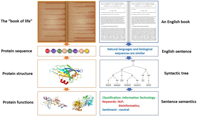
The genome is the ‘book of life’, whose languages are the biological sequences (1). Natural languages and biological sequences are similar. For examples, the peptide bonds connect the amino acid residues to form a protein with certain structure and function. Similarly, words are combined by grammar and linguistic rules into a sentence with certain meanings. In this regard, the techniques grounded in linguistics are used to uncover the meanings of the ‘book of life’, and have greatly contributed to the development of biological sequence analysis. Protein domains can be considered as the words of proteins, and the rules for domain associations are the grammar of proteins (2). Inspired by these similarities between proteins and languages, the linguistic technique n-gram was employed to probe the proteome grammar, showing that a ‘quasi-universal grammar’ underlies the evolution of domain architectures (3). Biological sequences store all the information determining their structures and functions, and the sentences contain all the information defining their syntactic and semantic (4). Because the relationships among biological sequence, structure and function are similar as the relationships among sentence, syntactic and semantic in linguistics (see Figure 1), techniques for semantic analysis derived from natural language processing have been applied to predict the structures and functions of proteins (5), providing new ideas and approaches for solving these tasks.

Figure 1.

The similarities between protein sequence and natural language sentence.

All these approaches based on natural language processing are playing important roles in uncovering the meanings of the ‘book of life’. Unfortunately, we still know only a little about its semantic. The existing studies focus on exploring the lexical, syntactic, or semantic of biological sequences. The biological sequences with various structures and functions share some common features with natural languages, but they also have their own linguistic properties. For examples, there are >500 physiochemical properties for amino acids (6), and >180 physiochemical properties for nucleotides (7). Even the most complicated polysemous word in a language will never have so many properties. As a result, the rule-based approaches show limited performance for some difficult tasks, such as protein disordered region prediction, enhancer identification, etc. Furthermore, these methods highly depend on the experience-based linguistic features. Therefore, models which are able to automatically and systematically capture the linguistic features are highly desired. They are critical for promoting the development of biological sequence analysis based on natural language processing. Language models can systematically and comprehensively represent and analyze the sentences, independent from the rule-based features, significantly contributing to the development of the natural language processing (8). Inspired by their successes, we are to propose the biological language models (BLMs) for DNA, RNA and protein sequences. Because the deep learning techniques have been demonstrated to be key methods in bioinformatics, such as protein structure prediction (9), and function analysis (10), BLMs mainly focuses on the biological neural language models to represent and analyze biological sequences based on deep learning techniques. We extend the BLMs to an automatic system called BioSeq-BLM (http://bliulab.net/BioSeq-BLM). Given the sequence data for a specific sequence analysis task, BioSeq-BLM will automatically construct the BLM, select the predictor, evaluate the performance, and analyze the results. BioSeq-BLM is particularly useful for solving the problems of extracting the linguistic features and designing the techniques derived from natural language processing, providing a new view to explore the meanings of ‘book of life’. It is anticipated that BioSeq-BLM will be a useful tool for biological sequence analysis, computational proteomics and genomics. As discussed in previous studies (11–13), a system which is able to automatically analyze the biological sequence data is highly desired, and several software tools have been established, such as BioSeq-Analysis (11), BioSeq-Analysis2.0 (12), protr (14), Rcpi (15), Kipoi (16), Janggu (17), Selene (18) and Pydna (19). However, among these existing tools, only BioSeq-BLM and BioSeq-Analysis2.0 are able to automatically construct the predictors with the benchmark datasets as the inputs. The other five tools focus on the individual steps, such as feature extraction, machine learning algorithm selection, or performance evaluation. The fundamental difference between BioSeq-BLM and other similar tools such as BioSeq-Analysis (12) is that BioSeq-BLM is the first study to define the BLMs and introduce 155 different BLMs for biological sequence analysis. Although some features or machine learning techniques also exist in BioSeq-Analysis2.0, BioSeq-BLM is the only existing tool for biological sequence analysis based on biological language models, providing new concepts and techniques for this very important field. These contributions make BioSeq-BLM unique, and more powerful than BioSeq-Analysis2.0. The comparisons between BioSeq-BLM and BioSeq-Analysis2.0 were listed in Table 1, from which we can see that BioSeq-BLM is beyond the reach of BioSeq-Analysis2.0 and any other similar tools.

Table 1.

The differences between BioSeq-BLM and BioSeq-Analysis2.0

Modules	Descriptions	BioSeq-BLM	BioSeq-Analysis2.0
BLMs	Number of BGLMs	58	51
	Number of BSLMs	48	0
	Number of BNLMs	41	0
	Number of BSSLMs	8	0
Predictor construction	Number of machine learning algorithms	9	3
	Number of deep learning algorithms	6	0
Performance evaluation	Number of evaluation metrics	10	6
Result analysis	Number of methods for normalization	4	0
	Number of methods for clustering	5	0
	Number of algorithms for feature selection	5	0
	Number of models for dimension reduction	3	0
Other	Support GPU-accelerate or not	Yes	No

Our main contributions are as follows:

• Based on the similarities between natural languages and biological sequences, we introduce the biological language models (BLMs) motivated by language models (LMs) in the field of natural language processing.

• We extend the BLMs into a platform called BioSeq-BLM, only requiring the benchmark datasets as inputs. The predictor will be automatically constructed and evaluated with the help of BioSeq-BLM. BioSeq-BLM is freely available at http://bliulab.net/BioSeq-BLM/.

• Experimental results showed that the predictors constructed by BioSeq-BLM are able to improve the predictive performance for some biological sequence analysis tasks.

MATERIALS AND METHODS

Biological sequence analysis tasks

The aim of biological sequence analysis is to computationally analyze the sequences of DNA, RNA and proteins so as to identify their structures, functions and their associations with diseases. Given a benchmark dataset S for a specific biological sequence analysis task with N sequences:

(1)

where B_i is the i-th biological sequence in S represented as:

(2)

where represents the j-th word (the words of biological sequences will be introduced in the following sections) in .

Biological sequence analysis tasks can be mainly divided into residue-level analysis and sequence-level analysis (12), aiming to identify the properties of each residue () and the whole sequence (), respectively. Their main difference is that the residue-level analysis treats each residue as a sample, while sequence-level analysis treats each biological sequence as a sample. For more information, please refer to (12). The BLMs will play key roles in these tasks, which will be introduced in the following sections.

Biological language models

The language model (LM) creates a statistical model for English sentences based on the Markov processes (20), which is a milestone in the field of natural language processing. LM determines the joint probability of a word sequence (21) so as to accurately represent and analyze the sentences. In this study, we are to propose the biological language models (BLMs) to represent and analyze the biological sequences following the ideas of LM. A BLM can be constructed for a specific task based on the corresponding benchmark dataset S (cf. Equation 1), represented as:

(3)

where is feature vector of the word in the sequence (cf. Equation 2), represented as:

(4)

where and are the linguistics attributes and biological attributes (such as physiochemical properties, etc) for , respectively.

Inspired by the success of language models (LMs) in the field of natural language processing, we introduce the biological language models (BLMs) for biological sequence analysis. The main differences between LM and BLM are as follows:

• Different inputs and methods. The inputs of LMs are sentences, while the inputs of BLMs are biological sequences. Furthermore, the words and word segmentation methods of BLMs are more diverse than those of LMs.

• More information in BLMs. BLMs not only consider the linguistic attributes of biological sequences, but also include the biological attributes, such as physical and chemical properties, evolutionary information, motifs, etc.

The proposed BLMs are able to capture both the linguistic features and biological properties, which can be further divided into four categories according to different computational techniques and theories, including biological grammar language models (BGLMs), biological statistical language models (BSLMs), biological neural language models (BNLMs), and biological semantic similarity language models (BSSLMs). These BLMs represent the biological sequences based on different techniques and theories, and are playing complementary roles in biological sequence analysis. These BLMs will be introduced in the following sections.

Biological grammar language models (BGLMs)

Natural languages present the meanings of their utterances structured according to their syntax, knowing as compositional semantics (22). In natural language processing, the grammar language models formally implement natural language understanding and generation based on grammar rules and linguistic knowledge. The biological sequences also have their own grammar rules, such as the motif associations (23), word relationships (24), word properties (6), etc. These grammar rules of biological sequences are important for insightfully representing the sequence characteristics. In this regard, 58 biological grammar language models (BGLMs) are used to represent and analyze the biological sequences. Among these 58 BGLMs, there are 29 models based on the syntax rules (see Table 2). Because the syntax rules reflect the relationships among residues along the biological sequences, these models are particularly useful for analyzing the structures and functions of biological sequences, such as protein disordered region prediction (25), splice site prediction (26), etc. Similar as sentences, biological sequences have their own words with more diverse properties reflecting evolutionary information, physicochemical values, structure information, etc. In order to incorporate the word properties into BGLMs, the other 29 BGLMs are based on word properties (12) (see Supplementary Table S9). Because these BGLMs based on word properties are able to capture the physicochemical properties of residues and the evolutionary information of biological sequences, they are suitable for analyzing the residue properties, sequence properties, and the evolutionary relationships, such as protein remote homology detection (27), N6-Methyladenosine Sites (28), etc.

Table 2.

29 BGLMs based on syntax rules

Category	Model	Description
DNA	DAC	Dinucleotide-based auto covariance (24)
	DCC	Dinucleotide-based cross covariance (24)
	DACC	Dinucleotide-based auto-cross covariance (24)
	TAC	Trinucleotide-based auto covariance (24)
	TCC	Trinucleotide-based cross covariance (24)
	TACC	Trinucleotide-based auto-cross covariance (24)
	MAC	Moran autocorrelation (104,105)
	GAC	Geary autocorrelation (104,106)
	NMBAC	Normalized Moreau-Broto autocorrelation (104,107)
	ZCPseKNC	Z curve pseudo k tuple nucleotide composition (108)
	ND	Nucleotide Density (26)
RNA	DAC	Dinucleotide-based auto covariance (24,47)
	DCC	Dinucleotide-based cross covariance (24,47)
	DACC	Dinucleotide-based auto-cross covariance (24,47)
	MAC	Moran autocorrelation (104,105)
	GAC	Geary autocorrelation (104,106)
	NMBAC	Normalized Moreau-Broto autocorrelation (104,107)
	ND	Nucleotide Density (26)
Protein	AC	Auto covariance (24,47)
	CC	Cross covariance (24,47)
	ACC	Auto-cross covariance (24,47)
	PDT	Physicochemical distance transformation (27)
	PDT-Profile	Profile-based physicochemical distance transformation (27)
	AC-PSSM	Profile-based Auto covariance (24)
	CC-PSSM	Profile-based Cross covariance (24)
	ACC-PSSM	Profile-based Auto-cross covariance (24)
	PSSM-DT	PSSM distance transformation (27)
	PSSM-RT	PSSM relation transformation (109)
	Motif-PSSM	Use PSSM as input and extract features by motifs-based CNN (23)

Biological statistical language models (BSLMs)

In linguistics, the statistical language models (SLMs) reflect statistical rules of languages by using the distribution functions based on the statistical principles (29). As a result, the underlying intentions and topics of languages can be discovered. Inspired by SLMs, the biological statistical language models (BSLMs) are introduced to recognize the statistical rules of biological sequences based on bag-of-words (BOW) (see Table 3), term frequency–inverse document frequency (TF-IDF) (30) (see Table 4), TextRank (31) (see Table 5), and topic models (32) (see Table 6). In this study, Kmer (33), RevKmer (33–35), Mismatch (36–38) and Subsequence (36,38,39) are treated as the words of DNA. Particularly, RevKmer is able to capture the characteristics of two strands of the double helix of DNA sequences. Kmer (40), Mismatch (36–38) and Subsequence (36,38,39) are considered as the words of RNA; Kmer (41), Mismatch (36–38), Top-n-gram (42), Distance Residue (DR) (43) and Distance Top-n-gram (DT) (43) are considered as the words of proteins. Please note that Top-n-gram and DT are the words with the evolutionary information. BOW model represents sentences as the ‘bag’ of words by word occurrence frequencies, ignoring grammar and word orders (44). Therefore, these BSLMs based on BOW are suitable for analyzing simple functions of biological sequences, such as human nucleosome occupancy prediction (34), gene regulatory sequence prediction (35), etc. TF-IDF model (45) reflects the importance of words to the biological sequences. TextRank (31), a graph-based ranking model, recognizes key sentences by ranking the criticality of sentences in the text, and assigns higher weights indicating the influence of a word. Because both the TF-IDF model and TextRank model are able to detect the key features of the biological sequences and reduce the dimensions of the feature vectors, they are suitable for constructing efficient predictors for sequence-level analysis tasks, such as RNA-binding protein prediction (46), protein–protein interaction prediction (47), etc. These three models are performed on the words of biological sequences, and generate 12 BSLMs based on BOW (see Table 3), 12 BSLMs based on TF-IDF (see Table 4) and 12 BSLMs based on TextRank (see Table 5). Furthermore, the topic model discovers the abstract ‘topics’ and the latent semantic structures of a ‘sequence document’ by using Latent Semantic Analysis (LSA) (48), Probabilistic Latent Semantic Analysis (PLSA) (32), Latent Dirichlet Allocation (LDA) (49) and Labeled-Latent Dirichlet Allocation (Labeled-LDA) (50), leading to 12 BSLMs based on topic models (see Table 6).

Table 3.

Twelve BSLMs based on BOW

Category	Model	Description
DNA	Kmer-BOW	Kmer-based BOW (33)
	RevKmer-BOW	Reverse-complementary- Kmer-based BOW (33–35)
	Mismatch-BOW	Mismatch-based BOW (36–38)
	Subsequence-BOW	Subsequence-based BOW (36,38,39)
RNA	Kmer-BOW	Kmer-based BOW (40)
	Mismatch-BOW	Mismatch-based BOW (36–38)
	Subsequence-BOW	Subsequence-based BOW (36,38,39)
Protein	Kmer-BOW	Kmer-based BOW (41)
	Mismatch-BOW	Mismatch-based BOW (37)
	DR-BOW	Distance-Residue-based BOW (43)
	Top-n-gram-BOW	Top-n-gram-based BOW (42)
	DT-BOW	Distance-Top-n-gram-based BOW (43)

Table 4.

Twelve BSLMs based on TF-IDF

Category	Model	Description
DNA	Kmer-TF-IDF	Kmer-based TF-IDF (30,33)
	RevKmer-TF-IDF	Reverse-complementary-Kmer- based TF-IDF (30,33–35)
	Mismatch-TF-IDF	Mismatch-based TF-IDF (30,36–38)
	Subsequence-TF-IDF	Subsequence-based TF-IDF (30,36,38,39)
RNA	Kmer- TF-IDF	Kmer-based TF-IDF (30,40)
	Mismatch-TF-IDF	Mismatch-based TF-IDF (30,36–38)
	Subsequence-TF-IDF	Subsequence-based TF-IDF (30,36,38,39)
Protein	Kmer-TF-IDF	Kmer-based TF-IDF (30,41)
	Mismatch-TF-IDF	Mismatch-based TF-IDF (30,37)
	DR-TF-IDF	Distance-Residue-based TF-IDF (30,43)
	Top-n-gram-TF-IDF	Top-n-gram-based TF-IDF(30,42)
	DT-TF-IDF	Distance-Top-n-gram-based TF-IDF (30,43)

Table 5.

Twelve BSLMs based on TextRank

Category	Model	Description
DNA	Kmer-TextRank	Kmer-based TextRank (31,33)
	RevKmer-TextRank	Reverse-complementary-Kmer- based TextRank (31,33–35)
	Mismatch-TextRank	Mismatch-based TextRank (31,36–38)
	Subsequence-TextRank	Subsequence-based TextRank (31,36,38,39)
RNA	Kmer-TextRank	Kmer-based TextRank (31,40)
	Mismatch-TextRank	Mismatch-based TextRank (31,36–38)
	Subsequence-TextRank	Subsequence-based TextRank (31,36,38,39)
Protein	Kmer-TextRank	Kmer-based TextRank (31,41)
	Mismatch-TextRank	Mismatch-based TextRank (31,37)
	DR-TextRank	Distance-Residue-based TextRank (31,43)
	Top-n-gram-TextRank	Top-n-gram-based TextRank (31,42)
	DT-TextRank	Distance-Top-n-gram-based TextRank (31,43)

Table 6.

Twelve BSLMs based on topic models

Algorithm	Model	Description
LSA	BOW-LSA	Latent Semantic Analysis (48)
	TF-IDF-LSA
	TextRank-LSA
LDA	BOW-LDA	Latent Dirichlet Allocation (49)
	TF-IDF-LDA
	TextRank-LDA
Labeled-LDA	BOW-Labeled-LDA	Labeled Latent Dirichlet Allocation Model (50)
	TF-IDF-Labeled-LDA
	TextRank-Labeled-LDA
PLSA	BOW-PLSA	Probabilistic Latent Semantic Analysis (32)
	TF-IDF-PLSA
	TextRank-PLSA

Biological neural language models (BNLMs)

In linguistics, the neural language models (NLMs) (51) employ deep neural networks to generate the distributed representations of words. Compared with other language models, the NLMs have the following advantages: (i) deep neural networks capture the local and global distance dependencies in a language; (ii) the distributed representation of words effectively avoids the problems of data sparse and dimensional disasters; (iii) the distributed representation of words captures the dependencies in a high-dimensional continuous space, leading to a better generalization ability. In order to incorporate these advantages into the biological language models, we introduce the biological neural language models (BNLMs) based on word embedding (Table 7) and automatic features (Table 8). Because linguistic objects with similar distributions have similar meanings (52), word embedding embeds each word into a continuous real-valued vector to represent the words. In this study, word2vec (53), GloVe (54) and fastText (55) are combined with the aforementioned words of biological sequences, and the corresponding 36 BNLMs based on word embedding are listed in Table 7. Deep learning techniques are able to automatically extract the linguistic features independent from grammar rules and other experience knowledge. Because deep learning techniques require sufficient samples to train the predictive models with high performance, BNLMs are suitable for analyzing both the residue-level and sequence-level tasks with enough training samples, such as protein structure prediction (9), protein fold recognition (56), disordered region prediction (57), etc. In this study, autoencoder (58), CNN-BiLSTM (56) and DCNN-BiLSTM (56) are used to model the dependencies among residues/words in biological sequences. MotifCNN (59) and MotifDCNN (59) are used to capture the motif-based features. Finally, five BNLMs based on automatic features are shown in Table 8.

Table 7.

Thirty-six BNLMs based on word embedding

Category	Algorithm	Model	Description
DNA	word2vec	Kmer2vec	Learn word representations via word2vec model (53)
		RevKmer2vec
		Mismatch2vec
		Subsequence2vec
	GloVe	Kmer-GloVe	Learn word representations via Glove model (54)
		RevKmer-GloVe
		Mismatch-GloVe
		Subsequence-GloVe
	fastText	Kmer-fastText	Learn word representations via fastText model (55)
		RevKmer-fastText
		Mismatch-fastText
		Subsequence-fastText
RNA	word2vec	Kmer2vec	Learn word representations via word2vec model (53)
		Mismatch2vec
		Subsequence2vec
	GloVe	Kmer-GloVe	Learn word representations via Glove model (54)
		Mismatch-GloVe
		Subsequence-GloVe
	fastText	Kmer-fastText	Learn word representations via fastText model (55)
		Mismatch-fastText
		Subsequence-fastText
Protein	word2vec	Kmer2vec	Learn word representations via word2vec model (53)
		Mismatch2vec
		DR2vec
		Top-n-gram2vec
		DT2vec
	GloVe	Kmer-Glove	Learn word representations via glove model (54)
		Mismatch-Glove
		DR-Glove
		Top-n-gram-Glove
		DT-Glove
	fastText	Kmer-fastText	Learn word representations via fastText model (55)
		Mismatch-fastText
		DR-fastText
		Top-n-gram-fastText
		DT-fastText

Table 8.

Five BNLMs based on automatic features

Model	Description
MotifCNN	CNN construction with motifs initializing convolution kernel (59)
MotifDCNN	DCNN construction with motifs initializing convolution kernel (59)
CNN-BiLSTM	Combine CNN and BiLSTM (56)
DCNN-BiLSTM	Combine DCNN and BiLSTM (56)
Autoencoder	Learning Sequence Representations based on Autoencoders (58)

Biological semantic similarity language models (BSSLMs)

Calculation of the sequence similarities of biological sequences is one of the keys in biological sequence analysis, which can be considered as the semantic similarities among sentences. The biological semantic similarity language models (BSSLMs) are able to represent the biological sequences based on the semantic similarities. The semantic similarities can be calculated by the feature vectors generated by the aforementioned three kinds of BLMs via Euclidean Distance (60–62), Manhattan Distance (63), Chebyshev Distance (64), Hamming Distance (65), Cosine Similarity (60–62), Pearson Correlation Coefficient (60–62), KL Divergence (Relative Entropy) (60–62), or Jaccard Similarity Coefficient (60–62). The resulting 8 BSSLMs are listed in Table 9. Because the BSSLMs are able to accurately calculate the similarities among biological sequences, they are suitable for analyzing the relationships among biological sequences and the associations between diseases and biological sequences, such as homology detection (60), non-coding RNA-disease association identification (66), etc.

Table 9.

Eight BSSLMs

Model	Description
ED	Euclidean Distance (60–62)
MD	Manhattan Distance (63)
CD	Chebyshev Distance (64)
HD	Hamming Distance (65)
CS	Cosine Similarity (60–62)
PCC	Pearson Correlation Coefficient (60–62)
KLD	KL Divergence (Relative Entropy) (60–62)
JSC	Jaccard Similarity Coefficient (60–62)

Extension of BLMs to BioSeq-BLM system

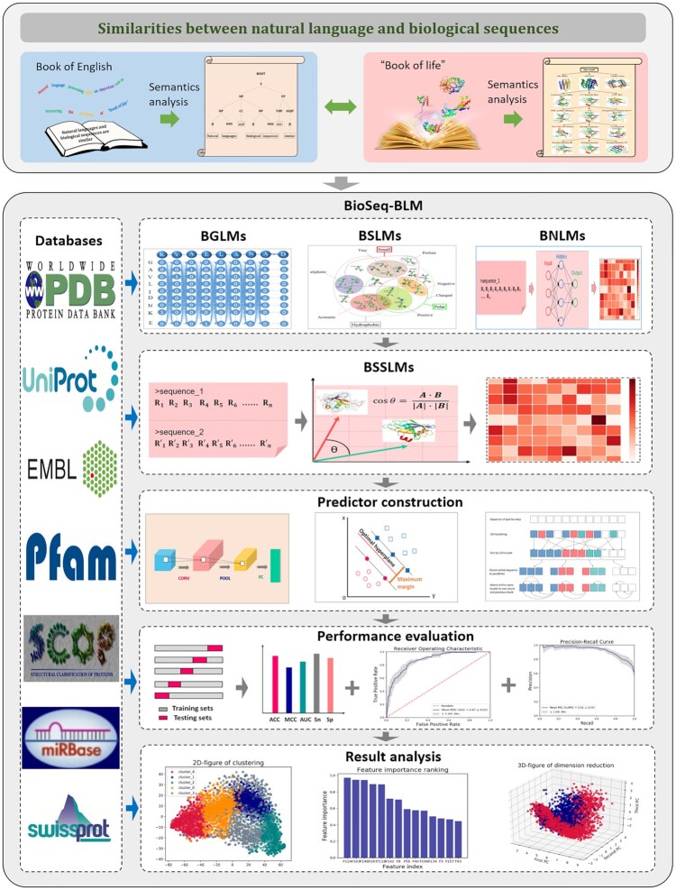
As introduced above, the BLMs represent the biological sequences in different aspects. We extend the BLMs to BioSeq-BLM system, making BLMs not only represent the biological sequences but also analyze the biological sequences, which is even out of the reach of any existing language model in linguistics. To achieve this goal, three other functions are added into BLMs, including predictor construction, performance evaluation, and result analysis, which will be introduced in the following sections. The overall flowchart of BioSeq-BLM is shown in Figure 2.

Figure 2.

The main components and their relationships of BioSeq-BLM. Inspired by the similarities between the natural languages and biological sequences, the BioSeq-BLM is constructed. There are four main components in BioSeq-BLM, including Biological Language Models (BLMs), predictor construction, performance evaluation and result analysis.

Predictor construction

We extend the BLMs to analyze the biological sequences by combining machine learning classifiers, which can be divided into three categories: classification algorithms, sequence labelling algorithm and deep learning algorithms.

For classification algorithms, the Support Vector Machine (SVM) (67) and Random Forest (RF) (68) are employed. They are widely used in classification tasks and regression tasks because of their good generalization ability (69). For the sequence labelling algorithm, the Conditional Random Field (CRF) (70) is used for the residue-level analysis tasks. Compared with the classification algorithms, CRF is able to model the biological sequences in a global fashion by considering the dependency information of all the residues along the sequences. For deep learning algorithms, the convolutional neural network (CNN) (57) captures the localized semantic association features. Long short-term memory (LSTM) (71) and Gated recurrent units (GRU) (72) capture the long-term dependence features of sequences. Transformer (73), weighted transformer (74) and reformer (75) capture the dependencies at any distances in sequences. Compared with the classification algorithms and sequence labelling algorithms, deep learning algorithms can learn the deeper representation of the sequences and model more complex interactions, leading to better performance for the sequence analysis task.

Performance evaluation

Here two methods are employed to evaluate the performance of BioSeq-BLM, including N-fold cross-validation and independent test. 9 metrics are used to measure the performance of BioSeq-BLM for binary classification tasks, calculated by:

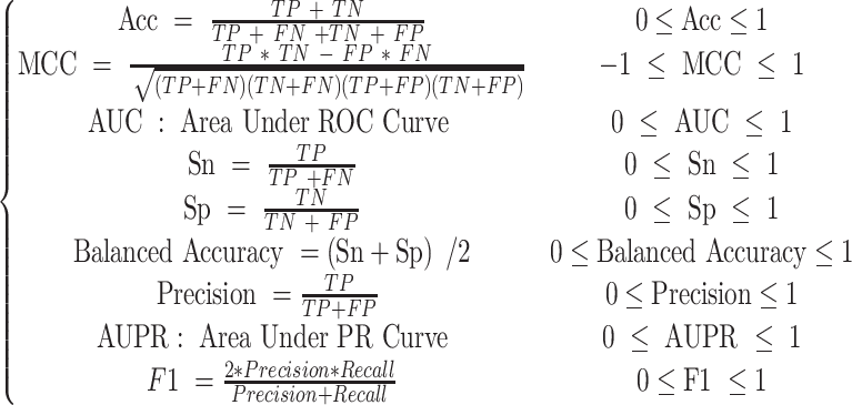(5)

where represents the number of true positive samples; represents the number of true negative samples; represents the number of false positive samples; represents the number of false negative samples. For multiclass classification tasks, multi-classification accuracy (12) is used, calculated by:

(6)

where represents the total number of the samples in the i-th class, is the number of the samples in the i-th class wrongly predicted as the other classes, represents the total number of the samples not in the i-th class and is the number of the samples not in the i-th class wrongly predicted to be the i-th class.

The selection of performance measures is generally based on the characteristics of datasets. For most biological sequence analysis tasks, Acc, MCC, AUC and Balanced Accuracy are the most commonly used metrics for performance evaluation. For a balanced dataset with approximately equal number of samples for each label, Acc metric can accurately evaluate the performance of a predictor. For an unbalanced dataset, MCC, AUC and Balanced Accuracy can better evaluate the performance of the predictors. For example, MCC and AUC are used to evaluate the performance of different predictors for identification of intrinsically disordered regions in proteins (76) because of the imbalance of samples.

BioSeq-BLM trained with imbalanced benchmark datasets will bias the class with fewer samples. In this regard, the sampling techniques are provided to solve this problem, including over-sampling method Synthetic Minority Oversampling Technique (SMOTE) (77), under-sampling method Tomek links (78) and the combination of over-sampling and under-sampling (79).

Result analysis

We provide a result analysis framework to interpret the predictive results with four modules: normalization, clustering, feature selection and dimension reduction. L1 regularization (80), L2 regularization (81), MinMaxScaler (82) and StandardScaler (82) in the normalization module can be used to normalize the features. Clustering module provides 5 cluster algorithms to visualize and validate if the corresponding BLM is able to accurately represent the data, including K-means (83), affinity propagation algorithms (84), Density-Based Spatial Clustering of Applications with Noise algorithm (DBSCAN) (85), Gaussian mixture model (86) and Agglomerative Nesting (87). Feature selection module provides 5 methods to analyze the importance of the features generated by BLMs, including chi-square (88,89), F-value (88,89), mutual information (88,89), recursive feature elimination (90) and tree mode (91). Three dimension reduction methods are incorporated into the dimension reduction module to remove the noise and reduce the dimensions of the feature vectors, including principal component analysis (PCA) (92), kernel principal component analysis (93) and truncated singular value decomposition (TSVD) (94).

BioSeq-BLM web server and stand-alone package

In order to help the researchers to use the biological language models for biological sequence analysis, we establish the web server and stand-alone tool of BioSeq-BLM, which can be freely accessed from http://bliulab.net/BioSeq-BLM/.

Web server

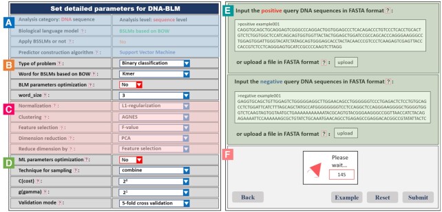
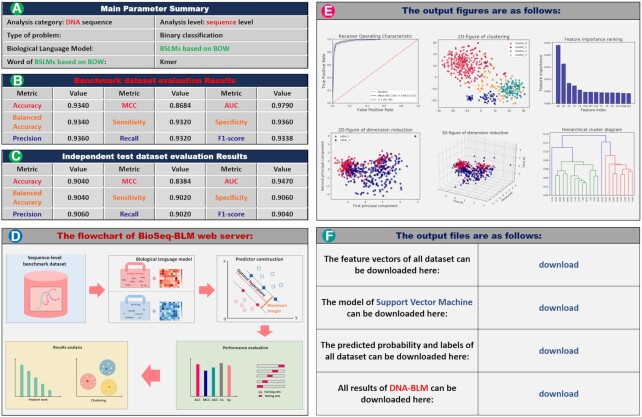
After clicking the ‘Server’ tab, three kinds of BLMs (DNA-BLM, RNA-BLM and protein-BLM for DNA, RNA and protein sequence analysis, respectively) will be shown on the screen, and then the level of analysis (residue-level analysis and sequence-level analysis) and BLM should be selected. Next, choose to calculate semantic similarity based on BSSLMs or not for sequence-level analysis. After selecting the machine learning algorithm, the submit page will be shown on the screen (see Figure 3A–D), where the users should set the parameters of the predictors, type the datasets in FASTA format into the input box or upload FASTA files (see Figure 3E and F). Finally click the ‘Submit’ for calculation. The results will be shortly shown on the screen (see Figure 4).

Figure 3.

Screenshot of the input page of BioSeq-BLM web server. (A) A summary of the main parameters; (B) the parameters for BLM; (C) the parameters of result analysis; (D) the parameters for predictor construction and performance evaluation; (E) the input box of the datasets; (F) the functional buttons.

Figure 4.

Screenshot of the result page of BioSeq-BLM web server. It contains six sections: (A) the summary of main parameters; (B) and (C) the evaluation results; (D) the flowchart; (E) the output figures; (F) the output files.

In this example, the BLM is set as Kmer-BOW (see Table 3) combined with the SVM for DNA sequence analysis at sequence level. The results page contains six parts as shown in Figure 4, from which the users can easily see the performance of the BLM and the importance of different features. This information is a key for selecting the BLM for biological sequence analysis. Please note that for BLMs based on deep learning techniques with high computational costs, the command lines of the stand-alone package will be given, based on which the users can easily obtain the corresponding results with the help of the stand-alone package installed in their own computers.

Stand-alone package

The web server of BioSeq-BLM is easy to use. However, for high-throughput analysis, its computational cost is high, especially for the BLMs based on deep learning techniques. In this regard, the stand-alone package of BioSeq-BLM is provided, which can be downloaded from http://bliulab.net/BioSeq-BLM/download/. Different from web server, the stand-alone package based on multithreading and GPU acceleration can make full use of local computing resources to implement computing. The trained models generated by BioSeq-BLM can be loaded to predict the unknown samples by using the stand-alone package of BioSeq-BLM. Furthermore, the bash scripts for automatically selecting the best models for specific biological sequence analysis tasks are incorporated into the stand-alone package, which will be particularly useful for biologists to choose the suitable models. For more information, please refer to the manual, which can be accessed at http://bliulab.net/BioSeq-BLM/static/download/BioSeq-BLM_manual.pdf.

How to choose web server or stand-alone package

The Stand-alone package and web server are complementary. The choice of web server and stand-alone package is related to the number of input sequences and the selected model. For a small number of sequences, web server is generally recommended. When there are many input sequences, it is recommended to use stand-alone package for calculation. If we need to use the model based on deep learning for biological sequence analysis, we suggest the users to use the web server to generate the command lines, and then use the corresponding command lines to run the stand-alone package. If users want to batch select the best BLM and machine learning algorithm for a specific task, the stand-alone package provides relevant scripts to facilitate the relevant functions.

RESULTS AND DISCUSSION

The BioSeq-BLM incorporates 155 different BLMs for biological sequence analysis. In this section, we will show how to use BioSeq-BLM to solve some specific biological sequence analysis tasks, which will be particularly helpful for researchers to select the BLMs.

Identification DNase I hypersensitive sites

Identification of DNase I hypersensitive sites (DHSs) is important for understanding the functions of noncoding genomic regions (95), which is a DNA sequence analysis task at sequence level. Here, we will show how to construct computational predictors for this task based on different BLMs and SVMs with the help of the stand-alone package of BioSeq-BLM. The benchmark dataset (95) downloaded from http://bliulab.net/iDHS-EL/data is used as the inputs of BioSeq-BLM. For example, a predictor Subsequence-BOW combines the BSLM of Subsequence-BOW (see Table 3) and SVM can be easily constructed with the help of the stand-alone package with the following command line:

python BioSeq-BLM_Seq.py -category DNA -mode BOW -words Subsequence -word_size 3 -cl Kmeans -nc 5 -fs F-value -nf 128 -rdb fs -ml SVM -sp combine -seq_file pos_file neg _file -label + 1 -1

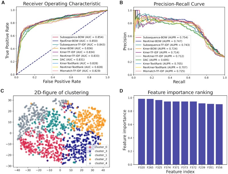
The performance of the top 10 best predictors generated by BioSeq-BLM is shown in Figure 5 and Supplementary Table S1, from which we can see that Subsequence-BOW predictor is highly comparable with the state-of-the-art predictor iDHS-EL reported in (95). The BOW model based on Subsequence words (36,38,39) is able to extract the discriminative features leading to better performance. All the complicated processes for constructing a computational predictor can be easily implemented by BioSeq-BLM with only one command line. Furthermore, the different BLMs incorporated in BioSeq-BLM would be potential candidates for constructing more efficient predictors for this task.

Figure 5.

(A) The Receiver Operating Characteristic (ROC) curves of top 10 predictors constructed by SVMs and different BLMs for identification DNase I hypersensitive sites; (B) the corresponding Precision-Recall (PR) curves of these 10 predictors; (C) the clustering results by K-means algorithm; (D) the 10 most important features and their corresponding feature importance values evaluated in terms of F-value.

Identification of real microRNA precursors

As miRNAs are deeply implicated with many cancers and other diseases, it is important for both basic research and miRNA-based therapy to discriminate the real pre-miRNAs from the false ones (96), which is a RNA sequence analysis task at sequence level. Given the benchmark dataset (96), the RSS predictor for miRNA prediction based on the BGLM of RSS (RNA Secondary Structure) (97) and SVM can be easily constructed with the help of BioSeq-BLM by using the following command line:

python BioSeq-BLM_Seq.py -category RNA -mode OHE -method RSS -cl Kmeans -nc 5 -dr TSVD -np 128 -rdb dr -ml SVM -seq_file pos_file neg _file -label + 1 -1

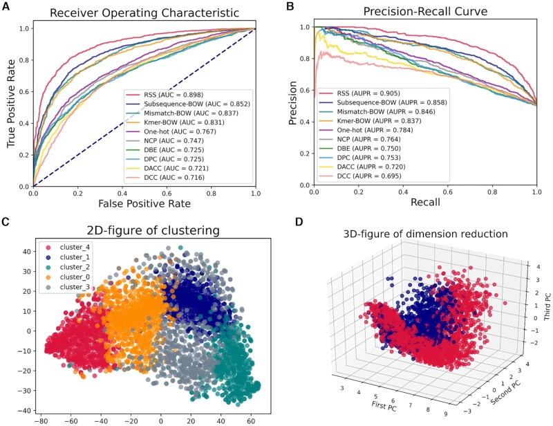
The performance of the top 10 best predictors generated by BioSeq-BLM is shown in Figure 6 and Supplementary Table S2. Because the BGLM of RSS can capture the ‘hairpin’ characteristics of miRNAs in their secondary structures, the computational predictor RSS generated by BioSeq-BLM achieves comparable performance with the iMcRNA predictor reported in (96), further confirming the usefulness of BioSeq-BLM for RNA sequence analysis.

Figure 6.

(A) The ROC curves of top 10 predictors constructed by SVMs and different BLMs for identification of real microRNA precursors; (B) the corresponding PR curves of these 10 predictors; (C) the clustering result for K-means algorithm; (D) the 3D-figure for dimension reduction when applying TSVD method.

Identification of DNA-binding proteins and RNA-binding proteins

Identification of DNA-binding proteins (DBPs) and RNA-binding proteins (RBPs) are important protein sequence analysis tasks at the sequence level. Identification of DBPs and RBPs play important roles in biological processes, such as replication, translation and transcription of genetic material.

A predictor BOW-LSA for DBP prediction can be generated by BioSeq-BLM by combining the BSLM of BOW-LSA (see Table 6) and RF with the following command line:

python BioSeq-BLM_Seq.py -category Protein -mode TM -method LSA -in_tm BOW -words Top-N-Gram -top_n 2 -com_prop 0.7 -cl Kmeans -nc 5 -fs Tree -nf 128 -ml RF -seq_file pos_file neg _file -label + 1 -1

A predictor PDT-Profile for RBP prediction can be generated by BioSeq-BLM by combining the BGLM of PDT-Profile (see Table 2) and SVM with the following command line:

python BioSeq-BLM_Seq.py -category Protein -mode SR -method PDT-Profile -ml SVM -seq_file pos_file neg _file -label + 1 -1

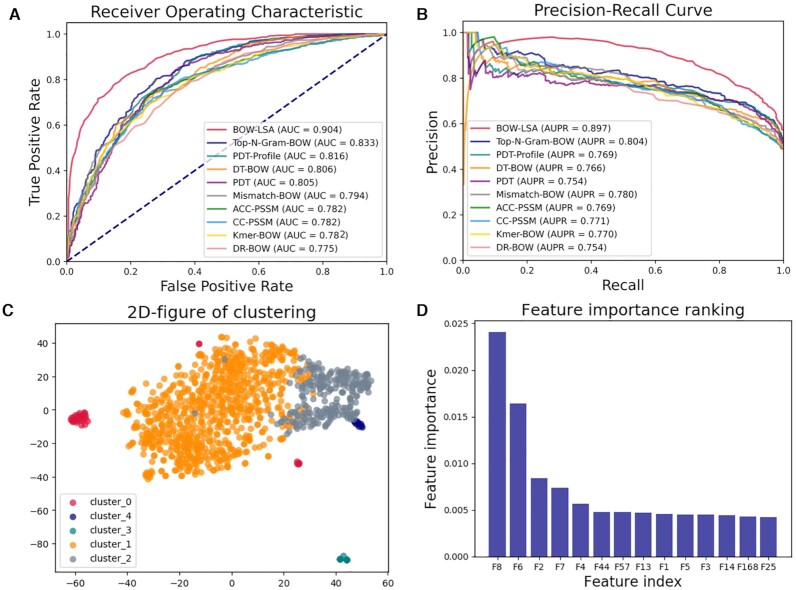
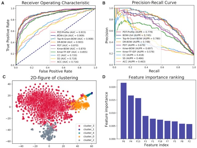
Evaluated on the benchmark dataset (98) for DBP identification, the performance of the top 10 best predictors generated by BioSeq-BLM is shown in Figure 7 and Supplementary Table S3. Because the BSLM of BOW-LSA is able to capture the global information, BOW-LSA shows the best performance and achieves an ACC of 81.58%, outperforming the predictor PseDNA-Pro reported in (98). Evaluated on the Salmonella benchmark dataset (46) for RBP identification, the performance of the top 10 best predictors generated by BioSeq-BLM is shown in Figure 8 and Supplementary Table S4. Because the BGLM of PDT-Profile (27) is able to efficiently extract the evolutionary information from the profiles, the PDT-Profile predictor combining PDT-Profile and SVM achieves the best performance with an AUC of 0.915, outperforming other three existing state-of-the-art predictors (TriPepSVM (46), RNAPred (99) and RBPPred (100)) by 6–13% in terms of AUC (see Supplementary Table S5). These results indicate that the predictors automatically generated by BioSeq-BLM can even achieve obviously better results than other existing approaches, which is another big step for the applications of the artificial intelligence to protein sequence analysis following the contributions of Alphfold2 (101) to the protein structure prediction.

Figure 7.

(A) The ROC curves of top 10 predictors constructed by RFs and different BLMs for identification of DNA binding proteins; (B) the corresponding PR curves of these 10 predictors; (C) the clustering result for K-means algorithm; (D) the 14 most important features and their corresponding feature importance evaluated by tree-based feature selection.

Figure 8.

(A) The ROC curves of top 10 predictors constructed by SVMs and different BLMs for identification of RNA binding proteins; (B) the corresponding PR curves of these 10 predictors; (C) the clustering result for K-means algorithm; (D) the 10 most important features and their corresponding feature importance evaluated by tree-based feature selection.

Identification of intrinsically disordered regions in proteins

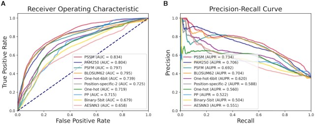
Intrinsically disordered regions (IDRs) in proteins are important for protein structure and function analysis, which is a protein sequence analysis task at residue level. BioSeq-Analysis2.0 (12) is another software tool based on machine learning techniques to automatically analyze biological sequences. In this regard, we compare the predictors constructed by BioSeq-BLM for IDR prediction with the predictors generated by BioSeq-Analysis2.0 on the benchmark dataset (76). A predictor PSSM for IDR prediction can be generated by BioSeq-BLM via combining the BLM of PSSM (102) and LSTM with the following command line:

python BioSeq-BLM_Res.py -category Protein -method PSSM -ml LSTM -epoch 10 -batch_size 20 -n_layer 2 -hidden_dim 64 -seq_file protein_seq_file -label_file protein_label_file

The performance of the top 10 predictors built by BioSeq-BLM is shown in Figure 9 and Supplementary Table S6. Because the LSTM captures the deep-level dependencies of residues in biological sequences in a global fashion, the PSSM predictor based on LSTM achieves the best performance among the 10 predictors. It also outperforms all the five top performing predictors generated by BioSeq-Analysis2.0 (12) by 8.7–12.6% in terms of AUC (see Supplementary Table S7). These results are not surprising because the BioSeq-BLM is based on the biological language models and deep learning methods, which are able to more accurately represent and analyze the biological sequences, and therefore, it achieves better performance than BioSeq-Analysis2.0.

Figure 9.

(A) The ROC curves of top 10 predictors constructed by LSTMs and different BLMs for identification of intrinsically disordered regions in proteins; (B) the corresponding PR curves of these 10 predictors.

RNA secondary structure prediction

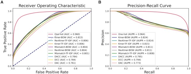
Identification of RNA secondary structure is an important step to understand RNA functions, which is a residue level analysis task. For example, we can use BioSeq-BLM to generate the One-hot predictor based on BGLM of One-hot and Random Forest by using the following command line:

python BioSeq-BLM_Seq.py -category RNA -mode OHE -method One-hot -ml RF -seq_file pos_file neg _file -label + 1 -1 -fixed_len 37

Given the benchmark dataset (PARS-Yeast dataset (103)), the performance of the top 10 predictors built by BioSeq-BLM is shown in Figure 10 and Supplementary Table S8. Because the combination of biological word properties and machine learning algorithms can improve the generalization ability of a predictor, the One-hot predictor achieves the best performance among the 10 predictors with an AUC of 0.960, which is highly comparable with the state-of-the-art predictor GRASP achieving an AUC of 0.967 (103).

Figure 10.

(A) The ROC curves of top 10 predictors constructed by RFs and different BLMs for RNA secondary structure prediction; (B) the corresponding PR curves of these 10 predictors.

CONCLUSION

As discussed above, the techniques derived from natural language processing (NLP) are the keys to uncover the meanings of the ‘book of life’. As a result, with the rapid growth of the biological sequence data, the NLP techniques are playing more and more important roles in prediction of the structures and functions of these sequence data. Unfortunately, it is never an easy task to find the suitable NLP techniques to solve a specific task. In order to solve this challenging problem, in this study, we introduce 155 different BLMs for DNA, RNA and protein sequence analysis, and extend these BLMs into a system called BioSeq-BLM, which is able to automatically represent and analyze the sequence data only requiring the sequence data in FASTA format as inputs. With its help, the predictors can be easily constructed. Experimental results show that the predictor even outperforms the existing state-of-the-art approaches for specific tasks. BioSeq-BLM provides new approaches for biological sequence analysis based on the techniques from NLP, which is particularly useful for constructing the computational predictors, or at the very least, it will play a commentary role with the existing methods to contribute to the development of this very important field.

Notes

Present address: Bin Liu, Beijing Institute of Technology, No. 5, South Zhongguancun Street, Haidian District, Beijing 100081, China.

SUPPLEMENTARY DATA

Supplementary Data are available at NAR Online.

FUNDING

National Key R&D Program of China [2018AAA0100100]; National Natural Science Foundation of China [61822306, 61861146002, 61732012]; Beijing Natural Science Foundation [JQ19019]. Funding for open access charge: National Key R&D Program of China [2018AAA0100100].

Conflict of Interest statement. None declared.

REFERENCES

- 1. Searls D.B. The language of genes. Nature. 2002; 420:211–217. [DOI] [PubMed] [Google Scholar]
- 2. Scaiewicz A., Levitt M.. The language of the protein universe. Curr. Opin. Genet. Dev. 2015; 35:50–56. [DOI] [PMC free article] [PubMed] [Google Scholar]
- 3. Yu L.J., Tanwar D.K., Penha E.D.S., Wolf Y.I., Koonin E.V., Basu M.K.. Grammar of protein domain architectures. Proc. Natl. Acad. Sci. U.S.A. 2019; 116:3636–3645. [DOI] [PMC free article] [PubMed] [Google Scholar]
- 4. Searls D.B. Reading the book of life. Bioinformatics. 2001; 17:579–580. [DOI] [PubMed] [Google Scholar]
- 5. Gimona M. Protein linguistics - a grammar for modular protein assembly?. Nat. Rev. Mol. Cell Biol. 2006; 7:68–73. [DOI] [PubMed] [Google Scholar]
- 6. Kawashima S., Pokarowski P., Pokarowska M., Kolinski A., Katayama T., Kanehisa M.. AAindex: amino acid index database, progress report 2008. Nucleic Acids Res. 2008; 36:D202–D205. [DOI] [PMC free article] [PubMed] [Google Scholar]
- 7. Friedel M., Nikolajewa S., Suhnel J., Wilhelm T.. DiProDB: a database for dinucleotide properties. Nucleic Acids Res. 2009; 37:D37–D40. [DOI] [PMC free article] [PubMed] [Google Scholar]
- 8. Chen Z., Eavani H., Chen W., Liu Y., Wang W.Y.. Few-Shot NLG with Pre-Trained Language Model. Proceedings of the 58th Annual Meeting of the Association for Computational Linguistics (ACL). 2020; 183–190. [Google Scholar]
- 9. Senior A.W., Evans R., Jumper J., Kirkpatrick J., Sifre L., Green T., Qin C., Zidek A., Nelson A.W.R., Bridgland A.et al.. Improved protein structure prediction using potentials from deep learning. Nature. 2020; 577:706–710. [DOI] [PubMed] [Google Scholar]
- 10. Alipanahi B., Delong A., Weirauch M.T., Frey B.J.. Predicting the sequence specificities of DNA- and RNA-binding proteins by deep learning. Nat. Biotechnol. 2015; 33:831–838. [DOI] [PubMed] [Google Scholar]
- 11. Liu B. BioSeq-Analysis: a platform for DNA, RNA and protein sequence analysis based on machine learning approaches. Brief. Bioinform. 2019; 20:1280–1294. [DOI] [PubMed] [Google Scholar]
- 12. Liu B., Gao X., Zhang H.Y.. BioSeq-Analysis2.0: an updated platform for analyzing DNA, RNA and protein sequences at sequence level and residue level based on machine learning approaches. Nucleic Acids Res. 2019; 47:e127. [DOI] [PMC free article] [PubMed] [Google Scholar]
- 13. Chen Z., Zhao P., Li F., Marquez-Lago T.T., Leier A., Revote J., Zhu Y., Powell D.R., Akutsu T., Webb G.I.et al.. iLearn: an integrated platform and meta-learner for feature engineering, machine-learning analysis and modeling of DNA, RNA and protein sequence data. Brief. Bioinform. 2019; 21:1047–1057. [DOI] [PubMed] [Google Scholar]
- 14. Xiao N., Cao D.S., Zhu M.F., Xu Q.S.. protr/ProtrWeb: R package and web server for generating various numerical representation schemes of protein sequences. Bioinformatics. 2015; 31:1857–1859. [DOI] [PubMed] [Google Scholar]
- 15. Cao D.S., Xiao N., Xu Q.S., Chen A.F.. Rcpi: R/Bioconductor package to generate various descriptors of proteins, compounds and their interactions. Bioinformatics. 2015; 31:279–281. [DOI] [PubMed] [Google Scholar]
- 16. Avsec Z., Kreuzhuber R., Israeli J., Xu N., Cheng J., Shrikumar A., Banerjee A., Kim D.S., Beier T., Urban L.et al.. The Kipoi repository accelerates community exchange and reuse of predictive models for genomics. Nat. Biotechnol. 2019; 37:592–600. [DOI] [PMC free article] [PubMed] [Google Scholar]
- 17. Kopp W., Monti R., Tamburrini A., Ohler U., Akalin A.. Deep learning for genomics using Janggu. Nat. Commun. 2020; 11:3488. [DOI] [PMC free article] [PubMed] [Google Scholar]
- 18. Chen K.M., Cofer E.M., Zhou J., Troyanskaya O.G.. Selene: a PyTorch-based deep learning library for sequence data. Nat. Methods. 2019; 16:315–318. [DOI] [PMC free article] [PubMed] [Google Scholar]
- 19. Pereira F., Azevedo F., Carvalho Â., Ribeiro G.F., Budde M.W., Johansson B.. Pydna: a simulation and documentation tool for DNA assembly strategies using python. BMC Bioinformatics. 2015; 16:142. [DOI] [PMC free article] [PubMed] [Google Scholar]
- 20. Shannon C.E. A mathematical theory of communication. Bell Syst. Tech. J. 1948; 27:379–423. [Google Scholar]
- 21. Goodman J. A bit of progress in language modeling. Comput. Speech Lang. 2001; 15:403–434. [Google Scholar]
- 22. Chomsky N. Three models for the description of language. IRE Trans. Inf. Theory. 1956; 2:113–124. [Google Scholar]
- 23. Zhang J., Chen Q.C., Liu B.. iDRBP_MMC: identifying DNA-binding proteins and RNA-binding proteins based on multi-label learning model and motif-based convolutional neural network. J. Mol. Biol. 2020; 432:5860–5875. [DOI] [PubMed] [Google Scholar]
- 24. Dong Q.W., Zhou S.G., Guan J.H.. A new taxonomy-based protein fold recognition approach based on autocross-covariance transformation. Bioinformatics. 2009; 25:2655–2662. [DOI] [PubMed] [Google Scholar]
- 25. Hanson J., Paliwal K.K., Litfin T., Zhou Y.. SPOT-Disorder2: improved protein intrinsic disorder prediction by ensembled deep learning. Genomics Proteomics Bioinformatics. 2019; 17:645–656. [DOI] [PMC free article] [PubMed] [Google Scholar]
- 26. Bari A.T., Golam M., Reaz M.R., Choi H.-J., Jeong B.-S.. DNA Encoding for Splice Site Prediction in Large DNA Sequence. Proceedings of the 18th International Conference on Database Systems for Advanced Applications. 2013; Berlin, Heidelberg: 46–58.Springer Berlin Heidelberg. [Google Scholar]
- 27. Liu B., Wang X.L., Chen Q.C., Dong Q.W., Lan X.. Using amino acid physicochemical distance transformation for fast protein remote homology detection. PLoS One. 2012; 7:e46633. [DOI] [PMC free article] [PubMed] [Google Scholar]
- 28. Qiang X., Chen H., Ye X., Su R., Wei L.. M6AMRFS: robust prediction of N6-methyladenosine sites with sequence-based features in multiple species. Front. Genet. 2018; 9:495. [DOI] [PMC free article] [PubMed] [Google Scholar]
- 29. Bahl L.R., Brown P.F., Souza P.V., Mercer R.L.. A tree-based statistical language model for natural language speech recognition. IEEE Trans. Acoust. Speech Signal Process. 1989; 37:1001–1008. [Google Scholar]
- 30. Zhang W., Yoshida T., Tang X.. A comparative study of TF*IDF, LSI and multi-words for text classification. Expert Syst. Appl. 2011; 38:2758–2765. [Google Scholar]
- 31. Mihalcea R., Tarau P.. Textrank: Bringing order into text. Proceedings of the 2004 conference on Empirical Methods in Natural Language Processing. 2004; Barcelona, Spain: 404–411.Association for Computational Linguistics. [Google Scholar]
- 32. Blei D.M. Probabilistic topic models. Commun. ACM. 2012; 55:77–84. [Google Scholar]
- 33. Chen W., Lei T.Y., Jin D.C., Lin H., Chou K.C.. PseKNC: a flexible web server for generating pseudo K-tuple nucleotide composition. Anal. Biochem. 2014; 456:53–60. [DOI] [PubMed] [Google Scholar]
- 34. Gupta S., Dennis J., Thurman R.E., Kingston R., Stamatoyannopoulos J.A., Noble W.S.J.P.C.B.. Predicting human nucleosome occupancy from primary sequence. PLoS Comput. Biol. 2008; 4:e1000134. [DOI] [PMC free article] [PubMed] [Google Scholar]
- 35. Noble W.S., Kuehn S., Thurman R., Yu M., Stamatoyannopoulos J.. Predicting the in vivo signature of human gene regulatory sequences. Bioinformatics. 2005; 21:I338–I343. [DOI] [PubMed] [Google Scholar]
- 36. El-Manzalawy Y., Dobbs D., Honavar V.. Predicting flexible length linear B-cell epitopes. Comput. Syst. Bioinformatics Conf. 2008; 7:121–132. [PMC free article] [PubMed] [Google Scholar]
- 37. Leslie C.S., Eskin E., Cohen A., Weston J., Noble W.S.. Mismatch string kernels for discriminative protein classification. Bioinformatics. 2004; 20:467–476. [DOI] [PubMed] [Google Scholar]
- 38. Luo L.Q., Li D.F., Zhang W., Tu S.K., Zhu X.P., Tian G.. Accurate prediction of transposon-derived piRNAs by integrating various sequential and physicochemical features. PLoS One. 2016; 11:e0153268. [DOI] [PMC free article] [PubMed] [Google Scholar]
- 39. Lodhi H., Saunders C., Shawe-Taylor J., Cristianini N., Watkins C.. Text classification using string kernels. J. Mach. Learn. Res. 2002; 2:419–444. [Google Scholar]
- 40. Lin H., Deng E.Z., Ding H., Chen W., Chou K.C.. iPro54-PseKNC: a sequence-based predictor for identifying sigma-54 promoters in prokaryote with pseudo k-tuple nucleotide composition. Nucleic Acids Res. 2014; 42:12961–12972. [DOI] [PMC free article] [PubMed] [Google Scholar]
- 41. Liu B., Liu F.L., Wang X.L., Chen J.J., Fang L.Y., Chou K.C.. Pse-in-One: a web server for generating various modes of pseudo components of DNA, RNA, and protein sequences. Nucleic Acids Res. 2015; 43:W65–W71. [DOI] [PMC free article] [PubMed] [Google Scholar]
- 42. Liu B., Wang X., Lin L., Dong Q., Wang X.. A discriminative method for protein remote homology detection and fold recognition combining Top-n-grams and latent semantic analysis. BMC Bioinformatics. 2008; 9:510. [DOI] [PMC free article] [PubMed] [Google Scholar]
- 43. Liu B., Xu J., Zou Q., Xu R., Wang X., Chen Q.. Using distances between Top-n-gram and residue pairs for protein remote homology detection. BMC Bioinformatics. 2014; 15:S3. [DOI] [PMC free article] [PubMed] [Google Scholar]
- 44. Harris Z.S. Distributional structure. Word. 1954; 10:146–162. [Google Scholar]
- 45. Ramos J. Using tf-idf to determine word relevance in document queries. Proceedings of the First Instructional Conference on Machine Learning. 2003; 242:New Jersey, USA: 133–142. [Google Scholar]
- 46. Bressin A., Schulte-Sasse R., Figini D., Urdaneta E.C., Beckmann B.M., Marsico A.. TriPepSVM: de novo prediction of RNA-binding proteins based on short amino acid motifs. Nucleic Acids Res. 2019; 47:4406–4417. [DOI] [PMC free article] [PubMed] [Google Scholar]
- 47. Guo Y.Z., Yu L.Z., Wen Z.N., Li M.L.. Using support vector machine combined with auto covariance to predict proteinprotein interactions from protein sequences. Nucleic Acids Res. 2008; 36:3025–3030. [DOI] [PMC free article] [PubMed] [Google Scholar]
- 48. Landauer T.K., Foltz P.W., Laham D. An introduction to latent semantic analysis. Discourse Processes. 1998; 25:259–284. [Google Scholar]
- 49. Blei D.M., Ng A.Y., Jordan M.I.. Latent dirichlet allocation. J. Mach. Learn. Res. 2003; 3:993–1022. [Google Scholar]
- 50. Ramage D., Hall D., Nallapati R., Manning C.D.. Labeled LDA: A supervised topic model for credit attribution in multi-labeled corpora. Proceedings of the 2009 Conference on Empirical Methods in Natural Language Processing. 2009; Singapore: 248–256.Association for Computational Linguistics. [Google Scholar]
- 51. Bengio Y., Ducharme R., Vincent P., Jauvin C.. A neural probabilistic language model. J. Mach. Learn. Res. 2003; 3:1137–1155. [Google Scholar]
- 52. HARRIS Z. Distributional Structure. Word. 1954; 10:142–146. [Google Scholar]
- 53. Mikolov T., Chen K., Corrado G., Dean J.. Efficient estimation of word representations in vector space. 2013; arXiv doi:07 September 2013, preprint: not peer reviewedhttps://arxiv.org/abs//1301.3781.
- 54. Pennington J., Socher R., Manning C.D.. Glove: Global vectors for word representation. Proceedings of the 2014 Conference on Empirical Methods in Natural Language Processing. 2014; 1532–1543.Association for Computational Linguistics. [Google Scholar]
- 55. Joulin A., Grave E., Bojanowski P., Mikolov T.. Bag of Tricks for Efficient Text Classification. Conference of the European Chapter of the Association for Computational Linguistics. 2017; 2:427–431. [Google Scholar]
- 56. Liu B., Li C.C., Yan K.. DeepSVM-fold: protein fold recognition by combining support vector machines and pairwise sequence similarity scores generated by deep learning networks. Brief. Bioinform. 2020; 21:1733–1741. [DOI] [PubMed] [Google Scholar]
- 57. Hanson J., Yang Y.D., Paliwal K., Zhou Y.Q.. Improving protein disorder prediction by deep bidirectional long short-term memory recurrent neural networks. Bioinformatics. 2017; 33:685–692. [DOI] [PubMed] [Google Scholar]
- 58. Lebret R., Collobert R.. “The Sum of Its Parts”: joint learning of word and phrase representations with autoencoders. 2015; arXiv doi:18 June 20155,preprint: not peer reviewedhttps://arxiv.org/abs/1506.05703.
- 59. Li C.C., Liu B.. MotifCNN-fold: protein fold recognition based on fold-specific features extracted by motif-based convolutional neural networks. Brief. Bioinform. 2020; 21:2133–2141. [DOI] [PubMed] [Google Scholar]
- 60. Ye X.G., Wang G.L., Altschul S.F.. An assessment of substitution scores for protein profile-profile comparison. Bioinformatics. 2011; 27:3356–3363. [DOI] [PMC free article] [PubMed] [Google Scholar]
- 61. Rangwala H., Karypis G.. Profile-based direct kernels for remote homology detection and fold recognition. Bioinformatics. 2005; 21:4239–4247. [DOI] [PubMed] [Google Scholar]
- 62. Mittelman D., Sadreyev R., Grishin N.. Probabilistic scoring measures for profile-profile comparison yield more accurate short seed alignments. Bioinformatics. 2003; 19:1531–1539. [DOI] [PubMed] [Google Scholar]
- 63. Strauss T., von Maltitz M.J.. Generalising Ward's method for use with Manhattan distances. PLoS One. 2017; 12:e0168288. [DOI] [PMC free article] [PubMed] [Google Scholar]
- 64. Weinberger K.Q., Saul L.K.. Distance metric learning for large margin nearest neighbor classification. J. Mach. Learn. Res. 2009; 10:207–244. [Google Scholar]
- 65. Laboulais C., Ouali M., Le Bret M., Gabarro-Arpa J.. Hamming distance geometry of a protein conformational space: application to the clustering of a 4-ns molecular dynamics trajectory of the HIV-1 integrase catalytic core. Proteins-Struct. Funct. Genet. 2002; 47:169–179. [DOI] [PubMed] [Google Scholar]
- 66. Wang L., You Z.H., Huang Y.A., Huang D.S., Chan K.C.C.. An efficient approach based on multi-sources information to predict circRNA-disease associations using deep convolutional neural network. Bioinformatics. 2020; 36:4038–4046. [DOI] [PubMed] [Google Scholar]
- 67. Chang C.C., Lin C.J.. LIBSVM: a library for support vector machines. ACM Trans. Intell. Syst. Technol. 2011; 2:27. [Google Scholar]
- 68. Biau G. Analysis of a random forests model. J. Mach. Learn. Res. 2012; 13:1063–1095. [Google Scholar]
- 69. Chen Z., Zhao P., Li C., Li F., Xiang D., Chen Y.Z., Akutsu T., Daly R.J., Webb G.I., Zhao Q.et al.. iLearnPlus: a comprehensive and automated machine-learning platform for nucleic acid and protein sequence analysis, prediction and visualization. Nucleic. Acids. Res. 2021; 49:e60. [DOI] [PMC free article] [PubMed] [Google Scholar]
- 70. Sutton C., McCallum A.. An introduction to conditional random fields. Found. Trends Mach. Learn. 2012; 4:267–373. [Google Scholar]
- 71. Hochreiter S., Schmidhuber J.. Long short-term memory. Neural Comput. 1997; 9:1735–1780. [DOI] [PubMed] [Google Scholar]
- 72. Cho K., van Merriënboer B., Gulcehre C., Bahdanau D., Bougares F., Schwenk H., Bengio Y.. Learning Phrase Representations using RNN Encoder–Decoder for Statistical Machine Translation. Proceedings of the 2014 Conference on Empirical Methods in Natural Language Processing. 2014; 1724–1734.Association for Computational Linguistics. [Google Scholar]
- 73. Vaswani A., Shazeer N., Parmar N., Uszkoreit J., Jones L., Gomez A.N., Kaiser Ł., Polosukhin I.. Attention is all you need. Proceedings of the 31st International Conference on Neural Information Processing Systems. 2017; Long Beach, California, USA: 6000–6010.Curran Associates Inc.. [Google Scholar]
- 74. Ahmed K., Keskar N.S., Socher R.. Weighted transformer network for machine translation. 2017; arXiv doi:06 November 2017, preprint: not peer reviewedhttps://arxiv.org/abs/1711.02132.
- 75. Kitaev N., Kaiser Ł., Levskaya A.. Reformer: the efficient transformer. 2020; arXiv doi:18 February 2020, preprint: not peer reviewedhttps://arxiv.org/abs/2001.04451.
- 76. Liu Y., Wang X., Liu B.. IDP–CRF: intrinsically disordered protein/region identification based on conditional random fields. Int. J. Mol. Sci. 2018; 19:2483. [DOI] [PMC free article] [PubMed] [Google Scholar]
- 77. Chawla N.V., Bowyer K.W., Hall L.O., Kegelmeyer W.P.. SMOTE: synthetic minority over-sampling technique. J. Artif. Intell. Res. 2002; 16:321–357. [Google Scholar]
- 78. Farquad M.A.H., Bose I.. Preprocessing unbalanced data using support vector machine. Decision Support Systems. 2012; 53:226–233. [Google Scholar]
- 79. Junsomboon N., Phienthrakul T.. Combining Over-Sampling and Under-Sampling Techniques for Imbalance Dataset. Proceedings of the 9th International Conference on Machine Learning and Computing. 2017; Singapore, Singapore: 243–247.Association for Computing Machinery. [Google Scholar]
- 80. Schmidt M., Fung G., Rosales R.. Fast Optimization Methods for L1 Regularization: A Comparative Study and Two New Approaches. Proceedings of the 18th European conference on Machine Learning. 2007; Warsaw, Poland: 286–297.Springer-Verlag. [Google Scholar]
- 81. Bilgic B., Chatnuntawech I., Fan A.P., Setsompop K., Cauley S.F., Wald L.L., Adalsteinsson E.. Fast image reconstruction with L2-regularization. J. Magn. Reson. Imaging. 2014; 40:181–191. [DOI] [PMC free article] [PubMed] [Google Scholar]
- 82. Pedregosa F., Varoquaux G., Gramfort A., Michel V., Thirion B., Grisel O., Blondel M., Prettenhofer P., Weiss R., Dubourg V.et al.. Scikit-learn: machine learning in Python. J. Mach. Learn. Res. 2011; 12:2825–2830. [Google Scholar]
- 83. Jain A.K., Murty M.N., Flynn P.J.. Data clustering: a review. ACM computing surveys. 1999; 31:264–323. [Google Scholar]
- 84. Frey B.J., Dueck D. Clustering by passing messages between data points. Science. 2007; 315:972–976. [DOI] [PubMed] [Google Scholar]
- 85. Ester M., Kriegel H.-P., Sander J., Xu X.. A density-based algorithm for discovering clusters in large spatial databases with noise. Proceedings of the Second International Conference on Knowledge Discovery and Data Mining. 1996; Portland, Oregon: 226–231.AAAI Press. [Google Scholar]
- 86. Kim S.C., Kang T.J.. Texture classification and segmentation using wavelet packet frame and Gaussian mixture model. Pattern Recogn. 2007; 40:1207–1221. [Google Scholar]
- 87. Skarmeta A.G., Bensaid A., Tazi N.. Data mining for text categorization with semi-supervised agglomerative hierarchical clustering. Int. J. Intell. Syst. 2000; 15:633–646. [Google Scholar]
- 88. Chandrashekar G., Sahin F.. A survey on feature selection methods. Comput. Electr. Eng. 2014; 40:16–28. [Google Scholar]
- 89. Guyon I., Elisseeff A.. An introduction to variable and feature selection. J. Mach. Learn. Res. 2003; 3:1157–1182. [Google Scholar]
- 90. Darst B.F., Malecki K.C., Engelman C.D.. Using recursive feature elimination in random forest to account for correlated variables in high dimensional data. BMC Genet. 2018; 19:353–363. [DOI] [PMC free article] [PubMed] [Google Scholar]
- 91. Sugumaran V., Muralidharan V., Ramachandran K.. Feature selection using decision tree and classification through proximal support vector machine for fault diagnostics of roller bearing. Mech. Syst. Signal Process. 2007; 21:930–942. [Google Scholar]
- 92. Yeung K.Y., Ruzzo W.L.. Principal component analysis for clustering gene expression data. Bioinformatics. 2001; 17:763–774. [DOI] [PubMed] [Google Scholar]
- 93. Schölkopf B., Smola A.J., Müller K.-R.. Kernel Principal Component Analysis. Proceedings of the 7th International Conference on Artificial Neural Networks. 1997; 583–588.Springer-Verlag. [Google Scholar]
- 94. Wei J.-J., Chang C.-J., Chou N.-K., Jan G.-J.. ECG data compression using truncated singular value decomposition. Trans. Info. Tech. Biomed. 2001; 5:290–299. [DOI] [PubMed] [Google Scholar]
- 95. Liu B., Long R., Chou K.C.. iDHS-EL: identifying DNase I hypersensitive sites by fusing three different modes of pseudo nucleotide composition into an ensemble learning framework. Bioinformatics. 2016; 32:2411–2418. [DOI] [PubMed] [Google Scholar]
- 96. Liu B., Fang L., Liu F., Wang X., Chen J., Chou K.-C.. Identification of real microRNA precursors with a pseudo structure status composition approach. PLoS One. 2015; 10:e0121501. [DOI] [PMC free article] [PubMed] [Google Scholar]
- 97. Hofacker I.L., Fontana W., Stadler P.F., Bonhoeffer L.S., Tacker M., Schuster P.. Fast folding and comparison of rna secondary structures. Monatsh. Chem. 1994; 125:167–188. [Google Scholar]
- 98. Liu B., Xu J.H., Fan S.X., Xu R.F., Zhou J.Y., Wang X.L.. PseDNA-Pro: DNA-binding protein identification by combining Chou's PseAAC and physicochemical distance transformation. Mol. Inf. 2015; 34:8–17. [DOI] [PubMed] [Google Scholar]
- 99. Kumar M., Gromiha M.M., Raghava G.P.S.. SVM based prediction of RNA-binding proteins using binding residues and evolutionary information. J. Mol. Recognit. 2011; 24:303–313. [DOI] [PubMed] [Google Scholar]
- 100. Zhang X., Liu S.. RBPPred: predicting RNA-binding proteins from sequence using SVM. Bioinformatics. 2017; 33:854–862. [DOI] [PubMed] [Google Scholar]
- 101. Callaway E. It will change everything’: DeepMind's AI makes gigantic leap in solving protein structures. Nature. 2020; 588:203–204. [DOI] [PubMed] [Google Scholar]
- 102. Altschul S.F., Koonin E.V.. Iterated profile searches with PSI-BLAST - a tool for discovery in protein databases. Trends Biochem. Sci. 1998; 23:444–447. [DOI] [PubMed] [Google Scholar]
- 103. Ke Y., Rao J., Zhao H., Lu Y., Xiao N., Yang Y.. Accurate prediction of genome-wide RNA secondary structure profile based on extreme gradient boosting. Bioinformatics. 2020; 36:4576–4582. [DOI] [PubMed] [Google Scholar]
- 104. Chen W., Zhang X., Brooker J., Lin H., Zhang L., Chou K.C.. PseKNC-General: a cross-platform package for generating various modes of pseudo nucleotide compositions. Bioinformatics. 2015; 31:119–120. [DOI] [PubMed] [Google Scholar]
- 105. Horne D.S. Prediction of protein helix content from an auto-correlation analysis of sequence hydrophobicities. Biopolymers. 1988; 27:451–477. [DOI] [PubMed] [Google Scholar]
- 106. Sokal R.R., Thomson B.A.. Population structure inferred by local spatial autocorrelation: an example from an Amerindian tribal population. Am. J. Phys. Anthropol. 2006; 129:121–131. [DOI] [PubMed] [Google Scholar]
- 107. Feng Z.P., Zhang C.T.. Prediction of membrane protein types based on the hydrophobic index of amino acids. J. Protein Chem. 2000; 19:269–275. [DOI] [PubMed] [Google Scholar]
- 108. Chen J.H., Liu Y.M., Liao Q., Liu B.. iEsGene-ZCPseKNC: identify essential genes based on Z curve pseudo k-tuple nucleotide composition. Ieee Access. 2019; 7:165241–165247. [Google Scholar]
- 109. Zhou J., Lu Q., Xu R., He Y., Wang H.. EL_PSSM-RT: DNA-binding residue prediction by integrating ensemble learning with PSSM relation transformation. BMC Bioinformatics. 2017; 18:379. [DOI] [PMC free article] [PubMed] [Google Scholar]
Associated Data
This section collects any data citations, data availability statements, or supplementary materials included in this article.