Flexible CDOCKER: Hybrid Searching Algorithm and Scoring Function with Side Chain Conformational Entropy

Abstract

The binding of small molecule ligands to protein or nucleic acid targets is important to numerous biological processes. Accurate prediction of the binding modes between a ligand and a macromolecule is of fundamental importance in structure based structure-function exploration. When multiple ligands with different sizes are docked to a target receptor, it is reasonable to assume that the residues in the the binding pocket may adopt alternative conformations upon interacting with the different ligands. In addition, it has been suggested that the entropic contribution to binding can be important. However, only a few attempts to include the side chain conformational entropy upon binding within the application of flexible receptor docking methodology exist. Here, we propose a new physics-based scoring function that includes both enthalpic and entropic contributions upon binding by considering the conformational variability of the flexible side chains within the ensemble of docked poses. We also describe a novel hybrid searching algorithm that combines both molecular dynamics (MD) based simulated annealing and genetic algorithm crossovers to address enhanced sampling of the increased search space. We demonstrate improved accuracy in flexible cross-docking experiments compared with rigid cross-docking. We test our developments by considering five protein targets, thrombin, dihydrofolate reductase(DHFR), T4 L99A, T4 L99A/M102Q and PDE10A, which belong to different enzyme classes with different binding pocket environments, as a representative set of diverse ligands and receptors. Each target contains dozens of different ligands bound to the same binding pocket. We also demonstrate that this flexible docking algorithm may be applicable to RNA docking with a representative riboswitch example. Our findings show significant improvements in top ranking accuracy across this set, with the largest improvement relative to rigid, 23.64%, occurring for ligands binding to DHFR. We then evaluate the ability to identify lead compounds among a large chemical space for the proposed flexible receptor docking algorithm using a subset of the DUD-E containing receptor targets MCR, GCR and ANDR. We demonstrate that our new algorithms show improved performance in modeling flexible binding site residues compared to DOCK. Finally, we select the T4 L99A and T4 L99A/M102Q decoy sets, containing dozens of binders and experimentally validated non-binders, to test our approach in distinguishing binders from non-binders. We illustrate that our new algorithms for searching and scoring have superior performance to rigid receptor CDOCKER as well as AutoDock Vina. Finally, we suggest that Flexible CDOCKER is sufficiently fast to be utilized in high-throughput docking screens in the context of hierarchical approaches.

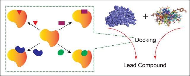
Graphical Abstract

INTRODUCTION

The development of new drugs with traditional methods can cost anywhere in the range of 400 million to 2 billion dollars, with synthesis and testing of lead analogs being a large contributor to that sum.¹ A successful in silico docking protocol can save a large amount of money and time, and this has been a focus of development in the field for decades. Generally speaking, docking predicts the orientation and conformation of a small molecule (ligand) in the binding site of the target protein and estimates its binding affinity.^2–4 Docking involves two main components: searching and scoring.³ In one element, searching, one generates multiple structures of a ligand within the constraints of the receptor binding site. The application of a scoring function, which can be classified as physics based, empirical or hybrid,^5–8 then ranks these conformations and is expected to differentiate the correct binding pose from incorrect ones through the assumption that the correct binding pose is at the top rank.

In high-throughput docking for hit identification, multiple small ligands with different sizes are docked to the target receptor. During this process, it is reasonable to assume the binding pocket undergoes conformational changes, and this has been captured experimentally.^9–12 Today, multiple off-the-shelf protein-ligand flexible docking programs, either commercial or free, are available for use, such as Glide,^13,14 ROSETTALIGAND,¹⁵ Flexible CDOCKER^16,17 and AutodockFR.¹⁸ As one notable example, the flexible docking method in Glide combines induced-fit docking and molecular docking (IFD-MD).^13,14 This method shows high accuracy in ranking native-like poses as top rank compared with rigid docking. However, the average computational cost for an IFD-MD calculation is 400 CPU hours and 50 GPU hours,¹⁴ which is similar to applications of AutodockFR, making it less likely to be applied in high-throughput experiments.

In a previous study we explored flexible receptor docking using the Seq17 dataset,¹⁸ which comprises 17 pairs of apo-holo structures that were selected to represent a wide range of receptors, both Flexible CDOCKER and AutodockFR showed a higher accuracy in finding a native-like pose compared with rigid docking.^17,18 However, both docking algorithms performed less well in ranking the native-like pose as top rank.^17,18 For Flexible CDOCKER with parallel simulated annealing running on one GPU, the average wall time required to compute the ensemble of ligand-receptor poses necessary to identify a cluster of native-poses for one protein-ligand complex was about 1hr, more than a 10-fold improvement in computing time compared to AutodockFR.¹⁷ Given this relatively high efficiency in finding a native-like pose in Flexible CDOCKER, in the current work we focus on further improvements in the search algorithm and on improving the scoring function for flexible docking.

Flexible CDOCKER¹⁶ uses a physics-based scoring function (eq 1) and does not include entropic contributions, which have been reported to be important in many cases.^19–22 Machine learning based scoring functions are constructed by characterizing protein-ligand complexes using feature vectors comprising the number of occurrences of specific protein-ligand atom type pairs interacting within predefined distance thresholds,^23,24 using different biochemical descriptors to characterize the protein-ligand interaction,²⁵ or assigning different weights to physics-based scoring functions.²⁶ Empirical scoring functions, such as X-SCORE, propose an additional term for the calculation of conformational entropy based on the number of rotatable bonds in the ligand.²⁷ However, both empirical approaches and machine learning based approaches may not serve to capture the side chain conformational entropy change upon binding because the number of the flexible side chain rotatable bonds does not change when binding to two different ligands. In the current work, we seek to improve the general physics-based scoring function by including an entropy calculation based on the microscopic definition of entropy as described below. We test this idea with a range of different datasets that include multiple receptors and ligands.

$$\mathrm{\Delta }{G}_{binding}=E_{proteininternalenergy}+E_{ligandinternalenergy}+E_{vdw}+E_{elec}$$ (1)

METHODS

CDOCKER Algorithm Overview

There are three main elements to the Flexible CDOCKER algorithm: the receptor and ligand representation, the newly developed scoring function, which includes the calculation of side chain conformational entropy, and a corresponding updated hybrid searching algorithm that combines molecular dynamics (MD) based simulated annealing^2,3,16,17,28 and genetic algorithm crossovers.^2,3,18,29,30 In the current study, the rigid docking algorithm and MD based simulated annealing parameters are the same as reported in our previous studies and are included in supplementary Table S1.^16,17

Receptor and Ligand Representation

All structure files were acquired from the PDB and had a structural resolution better than 2.0 Å. A complete list of the protein and RNA PDB codes are included in supplementary Table S2. MOE (Molecular Operating Environment)³¹ was used to predict the protonation state of the ligands and cofactor at pH 7.4. The dominant protonation state of the compound is selected for the following docking experiments. Open Babel³² was used to generate random ligand conformations, ParamChem^33,34 was used to prepare the ligand topology and parameter files and the MMTSB tool set³⁵ was used to cluster the binding poses. The ligand is minimized with CHARMM in vacuum before the docking experiments. Clustering used the tool cluster.pl with a 1 Å cutoff radius for the K-means clustering based on ligand heavy atom RMSD. In preparing each receptor for docking experiments, all co-crystal structures from the same receptor were superimposed to each other based on the backbone root-mean-square deviation of atomic positions (RMSD) using PyMOL³⁶ to provide a common reference frame. The CHARMM C36 force fields³⁷ were used and docking was performed in CHARMM³⁸ with the CHARMM/OpenMM parallel simulated annealing feature.¹⁷ The RMSD cutoff to identify native-like poses is set to be 2.5 Å for flexible docking and 2.0 Å for rigid docking, to be consistent with the evaluation criteria in the previous studies.^17,18,28 For completeness, in our cross-docking experiment, we record the pose prediction accuracy as a function of RMSD cutoff and report the results in supplementary Figures S2, S3 and S4.

The idea of flexible docking is to allow conformational changes of receptor side chains to occur so that the ligand can identify its native-like pose. Incorporation of protein flexibility has become more feasible due to advances in computational resources. In drug discovery, one often starts with one or a few co-crystal structures and uses flexible docking experiments to identify the native-like pose for ligands that do not yet have a co-crystal structure. To mimic this process, for each receptor-ligand holo complex in a cross-docking dataset with N crystal structures, we develop a unique definition of the flexible side chains for each receptor based on the distance between ligand heavy atoms and the corresponding target structure side chain atoms. We identified a receptor side chain as flexible if at least one pairwise interaction of the ligand heavy atoms and the side chain was within a 4Å cutoff.^17,18 All side chain atoms from the C-alpha carbon are considered flexible. For each complex used in this study, the receptor flexible residues are listed in the supplementary file (flexible-residues.xlsx). The average number of flexible side chains in this study is 10. The distribution of flexible side chains and rotatable bonds within the ligands are shown in Figure 1.

Figure 1:

Receptor binding pocket complexity. (A) Distribution of number of receptor flexible side chains. (B) Distribution of number of receptor rotatable bonds.

For the cross-docking experiment against a given receptor with flexible side chains defined as noted above, N − 1 ligands were docked to this structure with no changes in flexible side chain selections. The cross-docking experiments were performed for all N receptor structures, each with a potentially different set of flexible side chains depending on the bound ligand in that receptor. Thus, we have a total of N × (N − 1) cross-docking experiments for a dataset with N crystal structures. For completeness, we also report the N self-docking results as well. In the real application, we note that one could incorporate more structures with varied ligand interfaces to the receptor if they were available, thereby expanding the size of the flexible side chain region to accommodate the additional knowledge about the targeted receptor. If one does not have any knowledge of the bound state except a targeted binding pocket, one could perform some rigid docking trials to identify side chains that may interact with the ligands and choose the flexible region in this manner.

Benchmark Dataset

In high throughput screening, the more common case is that there exits a large number of different ligands docked to the same receptor. Thus, we use the 6 datasets shown in Table 1, which cover different receptor classes and binding environments. Each receptor contains several ligands. All co-crystal structures from the same receptor class share the same binding pocket. A brief description of the data sets and our rationale for choosing each is given in the following.

Table 1:

Receptor Dataset

Receptor Name	Co-crystal structures	Cross-docking/re-docking experiments	Receptor class
PDE10A	44	1892 / 44	Kinase
T4 L99A	23	506 / 23	Lysozyme
T4 L99A/M102Q	21	420 / 21	Lysozyme
DHFR	11	110 / 11	Folate enzyme
Thrombin	14	182 / 14	Serine protease
Riboswtich	4	12 / 4	RNA

T4 L99A dataset.

dataset was chosen to provide a simple model where the binding pocket is small, buried and hydrophobic and is comprised of a total of 23 different holo structures. It was chosen to test the performance of the flexible docking algorithm for the case of a small, buried and hydrophobic binding pocket.³⁹

T4 L99A/M102Q dataset.

This dataset is examined to provide a simple model where the binding pocket is small, buried and contains only one hydrophilic side chain.³⁹ It contains a total of 21 different holo structures. It has been included to test the performance of our flexible docking algorithm when the binding pocket that is small, buried and hydrophobic with only one hydrophilic side chain presented.

Riboswitch dataset.

Many research groups have developed different docking algorithms for RNA-ligand docking.^40–49 The common feature in these studies is that the majority of the investigated targets are complex, including large and flexible ligands and water-mediated interactions. These are still challenging in the current protein-ligand docking methodologies and make it difficult to distinguish these effects from issues specific to RNA-ligand flexible docking. Therefore, we selected a rather simple RNA-ligand docking system developed by the Brenk group, which allows us to focus on the impact of side chain flexibility on docking accuracy (i.e., backbone RMSD less than 2 Å).⁵⁰ There are only 4 different holo structures in this dataset. Compared with the two T4 datasets, this dataset also serves the purpose to test the performance of our flexible docking algorithm for cases of a small, buried and hydrophilic binding pocket.

PDE10A dataset.

This dataset contains 44 different holo structures of phosphodiesterase 10A (PDE10A), which is a kinase. There are either two nickel ions or one zinc ion and one magnesium ion included as part of the binding pockets. The nickel ions have not been parameterized in the CHARMM force field. Since all of the ions have a +2 charge and occupy similar positions in the binding pocket, we used the same zinc ion and magnesium ion in the cross-docking experiments. This dataset is built to test the performance of the flexible docking algorithm for cases where there are ions in the binding pocket.

DHFR dataset.

This dataset contains 11 different holo structures of dihydrofolate reductase (DHFR), which is a folate enzyme.³⁹ It has a more open binding site displaying both polar and apolar binding regions. Nine of the holo structures have a common cofactor NDP (NADPH dihydro-nicotinamide-adenine-dinucleotide phosphate). One of the holo structures (PDBID: 1DR3) has a slightly different cofactor TAP (7-thionicotinamide-adenine-dinucleotide phosphate). The other holo structure (PDBID: 2CD2) also has a slightly different cofactor NAP (NADP nicotinamide-adenine-dinucleotide phosphate). All of the cofactors occupy the same position near the binding pocket. To be consistent in the cross-docking experiments, we used the same cofactor NDP. The main purpose of including this set of structures was to increase the variability of our dataset and test our flexible docking algorithm when cofactors are present.

Thrombin dataset.

This dataset contains 14 different holo structures of thrombin, which is a serine protease.³⁹ The ligands from this dataset are the largest. The binding pocket is also more open than the others. This dataset is built to test our flexible docking algorithm with large ligands.

Flexible Docking Scoring Function with Side Chain Entropic Contributions

Upon binding, the change in free energy can be represented by eq 2. In cases of differentiating the correct binding pose from incorrect ones, the same ligand is docked to the receptor multiple times and generates multiple docking poses. Since the ligand and protein always start from the same initial state, G_initial will be the same for all trials. Thus, only G_final needs to be calculated for pose identification. The enthalpic contribution (H_final), including protein-ligand interactions, ligand internal energy and protein internal energy, have been well-established in the previous Flexible CDOCKER scoring function.^16,28 The entropic contribution (S_final) can be separated into contributions from solvation and conformational entropy. Since we consistently dock the same ligand to the same binding pocket in one measurement, we assume the solvation contribution is approximately the same for different docking poses, and we suggest that it can be neglected. Thus, the flexible scoring function can be simplified to eq 3:

$$\begin{gathered} \mathrm{\Delta }{G}_{binding}=G_{final}-G_{inital} \\ =H_{final}-H_{initial}-T\left(S_{final}-S_{initial}\right) \end{gathered}$$ (2)

$$\begin{gathered} \mathrm{\Delta }{G}_{binding}=E_{protein-ligandinteraction}+E_{proteininternalenergy} \\ +E_{ligandinternalenergy}-T{S}_{conformationalentropy} \end{gathered}$$ (3)

For a given flexible docking measurement, the docking poses are clustered based on the ligand heavy atoms. Thus, in one ligand cluster, all ligand conformations are similar to each other. Therefore, the conformational entropy of the ligand within that cluster is assumed to be zero. However, as shown in figure 2, the receptor side chains can adopt different conformations, which results in a non-zero side chain conformational entropy and a variation of enthalpy within one cluster. Here, we use the microscopic definitions to compute the side chain conformational entropy upon binding.

Figure 2:

2OUN flexible self-docking results using the flexible receptor docking algorithm. These two docking poses (pink) belong to the same cluster and are native-like docking poses. The corresponding flexible side chain GLU726 adopts two different conformations. The backbone atoms of the two GLU726 conformations are shown in orange, while the side chain atoms are shown in yellow and blue, respectively. The side chain amide groups adopt two different orientations.

Protein side chain conformational states.

The amino acid side chain conformational states can be classified by the dihedral angle of the rotamers, an idea originally used for computing side chain conformational entropy in protein unfolded states.⁵¹ Only the dihedral angle χ, involving four heavy atoms, is considered as a rotamer. The IUPAC-IUB convention is used to define trans (±180°), gauche− (g−,−60°) and gauche+ (g+,+60°) conformations for a rotamer.⁵² Gly, Ala and Pro are excluded. Because of the symmetry in the benzyl group and phenyl group in Phe and Tyr respectively, these two amino acids have χ₂ rotamer conformations of 2 instead of 3. The maximum number of states that one amino acid can access is listed in Table 2.

Table 2:

Number of Rotamer States for Each Amino Acid

Residue	Total number of dihedral angles, χi	Maximum number of states
Arg, Lys	4	81
Gln, Glu, Met	3	27
Asn, Asp, His, ILe, Leu, Trp	2	9
Phe, Tyr	2	6
Cys, Ser, Thr, Val	1	3

RNA side chain conformational states.

The increasing number of RNA crystal structures enables a structure-based approach to the discovery of new RNA-binding ligands,^53,54 and a number of RNA-ligand docking software, such as AutoDock,⁴¹ DOCK^41,49 and RiboDock,⁴⁵ are available. RNA can adopt different three dimensional structures that are critical for its function. Thus, it is important to consider receptor flexibility during docking. DOCK⁴⁹ rescores the docking poses with receptor side chains being flexible, and RiboDock⁴⁵ uses an ensemble of receptor structures to mimic the receptor flexibility. Here, we want to expand the application of our new flexible docking algorithm to RNA-ligand docking, which allows the receptor side chains and ligand configurations to explore their conformational space simultaneously.

We define the sugar and phosphate group in the nucleotide monophosphate as the backbone of RNA and the nucleobase is considered as the flexible side chain. Thus, only one dihedral angle χ is presented in all 4 bases. Instead of using the IUPAC-IUB convention, we rotate this dihedral angle and record the total energy for each nucleotide monophosphate. This result is shown in the supplementary information (in Figure S1) and the conformational states determined by this protocol are summarized in Table 3.

Table 3:

Conformational State Determined by Dihedral Angle, χ

Nucleotide monophsphate	State 1	State 2
ADE, GUA	−91 ∼ 175°	−180 ∼ −91° or 75 ∼ 180°
URA, CYT	−170 ∼ 137°	−180 ∼ −170° or 137 ∼ 180°

Final flexible docking scoring function.

For a specific side chain in a given ligand cluster of size N, the conformational entropy of this side chain is calculated using the microscopic definition of entropy (eq 4). The state of a side chain is a function of all dihedral angles in that side chain. Different side chains are considered independent of each other.

$$\begin{gathered} S_{sidechainconformation}=-k_B\sum _j{p}_{j}ln{p}_j \\ {p}_j=\frac{numberofsidechainsinstatej}{N} \\ statej=f\left\{{\chi }_1,{\chi }_2,\dots ,{\chi }_n\right\} \end{gathered}$$ (4)

As we mentioned above, differences in structural conformations result in a variation of enthalpy in one cluster. For the same cluster, the system can be treated as a classical and discrete canonical ensemble. Each docking pose in this cluster is one state. The probability of a docking pose in state j can be calculated based on its energy. Since the entropy for all ligands in a given cluster is a constant, we can simplify the partition function and calculate the ensemble average of the enthalpic contributions with the following equation (eq 5):

$$\begin{gathered} p_j=\frac{e^{-\beta \mathrm{\Delta }{G}_{binding\text{,}j}}}{{\sum }_i{e}^{-\beta \mathrm{\Delta }{G}_{binding\text{,}i}}}=\frac{e^{-\beta \left(H_j-T{S}_j\right)}}{{\sum }_i{e}^{-\beta \left(H_i-T{S}_i\right)}}=\frac{e^{-\beta H_j}{e}^{\beta T{S}_j}}{{\sum }_i{e}^{-\beta H_i}{e}^{\beta T{S}_i}}=\frac{e^{-\beta H_j}}{{\sum }_i{e}^{-\beta H_i}} \\ \overline{H}=\sum _j{p}_j{H}_j \end{gathered}$$ (5)

By using an ensemble average of the enthalpy, the minimum energy pose, which has the largest weight among the cluster members, will be chosen as the best individual (representative) of that cluster. Therefore, we reach the final equation (eq 6). The temperature is set to be 298K in all docking experiments in the current study.

$$\begin{gathered} \mathrm{\Delta }{G}_{binding}={\overline{E}}_{protein-ligandinteraction}+{\overline{E}}_{proteininternalenergy} \\ +{\overline{E}}_{ligandinternalenergy}+k_{B}T\sum _{allsidechains}\sum _j{p}_{j}ln{p}_j \end{gathered}$$ (6)

New Hybrid Searching Algorithm

To further augment sampling in the context of flexible receptor side chains, we propose a hybrid search algorithm for Flexible CDOCKER that combines molecular dynamics (MD) based simulated annealing^2,3,16,28 and a continuous genetic algorithm.^{2,3,18,29,30,55,56} In genetic algorithms, the genome is the set of variables to optimize. A given set of values for these variables comprises a docking solution and is called an individual. In this study, these variables are the coordinates of the ligand and flexible side chains of the receptor. Following the ideas of hyperplane sampling in a discrete genetic space, where each individual (potential solution) is considered to be a hyperplane and the competition among different hyperplanes is reflected by the population⁵⁵, we cluster the docking poses and each cluster is considered to be a hyper-surface partially specified by the coordinates of the ligands, where the size of the cluster reflects the competition among different hyper-surfaces. The clustering we perform identifies common basins in the docking energy landscape of the ligand by identifying the clusters of ligands possessing similar positions and configurations, determined by clusters based on the ligand heavy atom RMSD with a radius cutoff of 1 Å. We combine the MD based simulated annealing algorithm to optimize the results by local minimization and redistributing the population of different hyper-surfaces by crossing genes comprised of ligand positions and conformations and flexible side chain conformations. The overall workflow is shown in Figure 3.

Figure 3:

Flexible docking searching algorithm.

Each docking measurement creates 500 individuals (these comprise the docking trials). The Open Babel functionality (obrotamer), which uses a genetic algorithm to perform a systematic search over all ligand rotatable bonds, is used to create a starting library of diverse conformers.³² This library of randomly generated conformers is then centered at the binding pocket followed by a random translation (maximum ± 2 Å) and random rotation (maximum 360°) to generate the initial ligand coordinates. An energy cutoff is applied to filter out significant collisions between ligand atoms and protein atoms due to the random translation and rotation.¹⁷ The receptor flexible side chains are initialized with the coordinates from the input conformation of the receptor. Then these individuals are optimized by a MD based simulated annealing algorithm. The docking poses (optimized individuals) are then K-means clustered based on ligand heavy atom RMSD with a radius cutoff of 1 Å. The top 10 largest clusters are scored with the scoring function described above. Since these optimized individuals could include docking poses that are outside of the binding pocket (i.e., large RMSD with respect to the (unknown) binding pose). We adopt the idea of “promising area” and “intensification” from the continuous genetic algorithm purposed by Chelouah.⁵⁶ The genetic algorithm and clustering method are performed to localize multiple local minima in the docking energy landscape (promising area), including (potentially) the global minima (native-like poses). The key concept of intensification is the concentrating of potential optimal solutions. To test this idea we examined the distribution of ligand RMSD with respect to the native pose for each of the ligands associated with the 6 receptors listed in Table 1 following the initial application of MD-based simulated annealing.

As shown in Figure 4, the less populated clusters are frequently away from the binding pocket. For simple systems (i.e., Riboswitch, T4 L99A and T4 L99A/M102Q) where the binding pocket is small and buried, the sampling space is small and the majority of the docking poses are native-like and clustered into the top 10 largest clusters. For complex systems (i.e., DHFR, PDE10A and Thrombin) where the binding pocket is more open and the ligands are larger, the sampling space is large and the ligand has a greater probability of adopting an incorrect binding pose that is away from the binding pocket. Regardless, the top 10 largest clusters contain the majority of the native-like poses. There is a small percentage of the less populated clusters that also contain native-like poses (i.e., within 2.5 Å RMSD cutoff of the native binding pose). This is because the RMSD cutoff for clustering is set to be 1 Å so that not all of the native-like poses are grouped into one large cluster. However, it is safe to select best individuals from the top 10 largest clusters as the “promising area” to construct the next generation of individuals.

Figure 4:

Average RMSD distribution of ligand docking poses in the initial generation. The RMSD values are binned with a 0.5 increment.

Intensification.

The minimum energy pose for each cluster is considered as the best individual of a cluster. We select the best individuals from the top 10 clusters as the parents. We first select 250 pairs of the individuals randomly using a roulette-wheel selection method. The probability of selecting a given parent is based on the population of the clusters (eq 7).

$$\begin{gathered} P_{select,i}=\frac{N_i}{{\sum }_{j=1}^{10}{N}_j} \\ {N}_i\text{,}\text{Population}\text{of}\text{solution}\text{j} \end{gathered}$$ (7)

The first intensification is done by performing a crossover that swaps the ligand-receptor pair to produce the intermediate generation. The probability for a pair of parents to undergo crossover is 0.5. The second intensification is mutation. The mutation operator in our hybrid searching algorithm is defined as a random translation (maximum 2 Å) and rotation (maximum 30°) of the ligand. The idea of the mutation operator is to find a lower energy state for the receptor-ligand pair. The probability of mutation for a given individual in the intermediate generation is a function of the difference between the total energy of that individual and the largest total energy value among the 10 parents (E_{cutoff, 1}) (eq 8).

$$\begin{gathered} E_{cutoff,1}=max\left\{E_{parent}\right\} \\ E=E_{crossover}-E_{cutoff} \\ {P}_{(E)}=\{\begin{array}{ll}1-0.5\times exp(E),\hfill & \mathrm{i}\mathrm{f}E<0.\hfill \\ 0.5\times exp(-E),\hfill & \mathrm{otherwise}\hfill \end{array} \end{gathered}$$ (8)

Therefore, the more stable a given individual is, the less likely it is to undergo a mutation. The acceptance of this mutation is iterative and an energy cutoff of the total energy is applied to avoid collision with the receptor resulting from crossover and mutation. If the energy cutoff is reached for a given individual then another mutation will be applied to this individual until the system energy is lower than the cutoff value. This energy threshold is calculated by adding 500 kcal/mol to E_{cutoff, 1}. This step allows us generate a new generation around the previously found “promising area” and the search around the best individuals from the previous generation.

Termination criteria.

One disadvantage of using the genetic algorithm is the number of generations (time) needed for the search to converge.⁵⁵ Currently, Flexible CDOCKER requires 1 hr for 500 docking trials (one generation) on a GPU¹⁷ and AutodockFR requires on average of 7.3 hr for one generation on a CPU.¹⁸ AutodockFR considers the solutions within 2 kcal/mol of the lowest energy solution as the “promising area” and performs an iterative genetic search so that all solutions will result in this focused sampling space, which by default uses 50 rounds of genetic evolution.¹⁸

However, as we mentioned before, the majority of the native-like poses are clustered into a small number of populated clusters and are considered as “promising areas”, and the following intensification step concentrates the individuals (potential solutions) in the next generation within this focused sampling space. Therefore, our searching algorithm requires fewer generations before the population of native-like poses reaches a plateau. This is more feasibly applied in practical applications, such as high-throughput virtual screening. Thus, we performed flexible docking experiments with 5 generations and recorded the population of native-like poses for each generation for all 6 different receptors. As shown in Figure 5, for all 6 datasets, the average population of native-like poses reaches a plateau after the second generation using the move set and gene construction we employ here. Therefore, we use 2 generations in our searching algorithm in the following experiments, which provides a sufficient population of native-like poses within a reasonable timeframe.

Figure 5:

Average population of native-like poses vs generation. Population for each docking measurement is calculated by dividing number of native-like poses by 500 (the number of trials in a generation). Average population of native-like poses for all 6 datasets is plotted with their corresponding error bars constructed by computing the standard deviation.

RESULTS

Flexible Docking vs Rigid Docking

We have demonstrated that our purposed flexible docking algorithm generates solutions of well-populated native-like poses in a highly competitive timeframe. The search of the optimal orientation (i.e., bound conformation) and ranking it as top rank is the fundamental objective of docking.^26,57 Now, we consider the following two questions: (1) Compared with rigid docking, does flexible docking improve in cross-docking native-pose identification? (2) In representative realistic applications, can we identify limitations that suggest areas for future improvement? To assess these questions, we performed cross-docking calculations on the 6 receptor datasets listed in Table 1 with the proposed flexible docking algorithm. Rigid CDOCKER and AutoDock Vina are used for direct comparison.

Datasets containing T4 L99A, T4 L99A/M102Q and the Riboswitch.

These three datasets provide simple binding environments: a hydrophobic environment, a hydrophobic environment with one hydrophilic side chain and a hydrophilic environment. All of the binding pockets are small and buried.^39,50 The ligands bound to those receptors are also small and rigid compared with ligands in other datasets as illustrated in Figure 6. The cumulative docking accuracy for flexible docking and rigid docking trials is illustrated in Figure 6 A–C. Top ranking accuracy of pose prediction is shown in Table 4.

Figure 6:

Cumulative docking accuracy for the (A) T4 L99A dataset, the (B) T4 L99A/M102Q dataset and the (C) Riboswitch dataset. Distribution of ligand properties: (D) rotatable bonds, (E) logP and (F) molecular weight. A rank of N means the correct docking pose is within the top N solutions. AutoDock Vina trials use an exhaustiveness of 20. Rigid CDOCKER uses 500 docking trials for each cross-docking experiment.

Table 4:

Top Rank Accuracy in Pose Prediction of Cross-docking/Re-docking

Receptor Name	Flexible CDOCKER	Rigid CDOCKER	AutoDock Vina
T4 L99A	66.21% / 82.61%	56.13% / 60.87%	49.01% / 47.83%
T4 L99A/M102Q	77.62% / 61.90%	54.29% / 80.95%	51.19% / 80.95%
Riboswitch	25.00% / 50.00%	41.67% / 50.00%	41.67% / 50.00%

As shown in Figure 6 and Table 4, flexible docking overall performs better than rigid docking. The top 10 ranking accuracy is above 98% for both T4 datasets. The largest improvement in top rank accuracy is for the T4 L99A/M102Q dataset, which is 23.33% higher than Rigid CDOCKER. This result suggests that flexible docking performs better when there exists differences in the binding environment that increases the specificity. The top ranking accuracy for both flexible docking and rigid docking is lower compared with the other two datasets for the Riboswitch. Two main differences between proteins and RNA in binding are:⁵⁰ (1) RNA molecules are highly charged and (2) RNA-ligand interactions are dominated by polar contacts. In the current docking setup, the docking scoring function uses a distance dielectric constant set to 3r.^16,28,58 This reduces the electrostatic interactions, which are the main interactions in RNA-ligand recognition. Studies have shown that using optimized force-field parameters for RNA-ligand docking could improve accuracy.⁵⁰ This could be a potential solution to the relatively lower top rank accuracy in the Riboswitch dataset and will be further explored in more focused studies of RNA-based targets but are beyond the scope of our current study.

Datasets containing PDE10A, DHFR and Thrombin.

We next move on to evaluate the flexible docking algorithm with three more complex systems: PDE10A dataset, DHFR dataset and thrombin dataset. All of these systems have a more open binding pocket. The PDE10A dataset has two ions within the binding site, while the DHFR dataset has a cofactor in the binding pocket. The ligands in the thrombin dataset are larger and more flexible than ligands we tested in the other datasets as illustrated in Figure 7. The ions or the cofactors are implicitly represented by the grids, but are present within the context of our physics based scoring function used to compute the receptor grid. The cumulative docking accuracy of both flexible docking and rigid docking calculations is shown in Figure 7 A–C. Top ranking accuracy of pose prediction is listed in Table 5.

Figure 7:

Cumulative docking accuracy for the (A) PDE10A dataset, the (B) DHFR dataset and the (C) Thrombin dataset. Distribution of ligand property: (D) rotatable bonds, (E) logP and (F) molecular weight. A Rank of N means the correct docking pose is within the top N solutions. AutoDock Vina trials use an exhaustiveness of 20. Rigid CDOCKER uses 500 docking trials for each cross-docking experiment.

Table 5:

Top Rank Accuracy in Pose Prediction of Cross-docking/Re-docking

Receptor Name	Flexible CDOCKER	Rigid CDOCKER	AutoDock Vina
PDE10A	36.84% / 50.00%	18.92% / 47.72%	6.87% / 31.82%
DHFR	50.91% / 54.54%	27.27% / 36.36%	17.27% / 54.54%
Thrombin	40.11% / 50.00%	32.42% / 50.50%	8.24% / 14.28%

We again see better performance for flexible docking compared to the rigid docking. The ranking results show that our proposed flexible docking algorithm works well for these complex systems. Having ions or cofactors does not appear affect the performance of the purposed flexible docking algorithm. The largest improvement in the top rank accuracy is observed in the DHFR dataset, which is 23.64% higher than rigid docking. The relatively low performance for the AutoDock Vina against the PDE10A could result from the fact that it does not support metal ions.

Impact of ligand initial placement on pose prediction accuracy.

One general problem in docking is how to place the ligand in the vicinity of the binding site and what initial ligand internal conformation to choose. The initial conformation and position of a ligand might be in an unfavorable configuration relative to the binding site (i.e., incorrect orientation or conformation). Due to the size of the large ligands, instead of adopting the correct conformation and reorienting in the binding pocket, they often need to leave the binding pocket, reorient the conformation and re-enter the binding pocket. This is very unlikely because of the relatively abbreviated sampling schedules required to make high-throughput docking feasible, and is evident from the decrease in pose prediction accuracy for systems with more flexible and large ligands as shown in Figure 6 and Figure 7 for all three docking algorithms. To explore the impact of searching exhaustiveness of ligand conformational space in docking, we designed and performed another set of flexible and rigid cross-docking experiments for the DHFR and Thrombin datasets. In this test, half of the docking trials (250 docking poses) in the initial generation had the ligand start with an internal conformation that matched that of the native bound conformation, followed by the random rotation and translation in docking with Flexible CDOCKER and Rigid CDOCKER, while the remaining initial configurations were chose as described earlier using obrotomer. For AutoDock Vina, half of the initial ligand configurations matched the native ligand’s conformation and the other half was randomly distributed.

As is clear from Figure 8, by having some of the ligands starting with the native internal conformation, we observed improved accuracy in pose prediction for all three docking methods. It is surprising that ligand internal conformation also affects the docking performance of AutoDock Vina, however, the results are clear. In real-world applications, the correct conformation will not be known beforehand. This suggests that either better methods to choose a ligand’s initial conformation and placement in the binding site, or the use of more extensive sampling may improve docking results for large flexible ligands. This is not a surprising result because the sampling space for highly flexible ligands is large and complex, and alternative approaches for ligand initial conformation picking and placement in the binding pocket are a topic of ongoing exploration.

Figure 8:

Cumulative docking accuracy for the (A) DHFR dataset and the (B) Thrombin dataset with some ligands starting with their native pose internal conformations. Top rank pose prediction accuracy of flexible docking is 74.54% and 74.18% using the proposed flexible receptor docking algorithm for each dataset, respectively.

Discriminating Binders from Non-binders

In a real application for lead compound discovery, one typically would face two questions: (1) For a given target with no knowledge of any inhibitors, how well does a docking method identify novel lead compounds within a large chemical space? If we have already identified several inhibitors for a specific target, one would expect that the derivatives of these known inhibitors could contain binders and non-binders for this target. (2) Then the question becomes how well does a docking method perform in discriminating binders from non-binders among the derivatives? To examine the effectiveness of our new sampling and scoring methods in distinguishing non-binders from binders, we perform flexible docking experiments against both ligands and non-binding decoys. The area under the curve (AUC) value of the receiver operating characteristic (ROC) curve is used to evaluate the performance in distinguishing the non-binders from binders.⁵⁹

Scoring function.

In order to compare different small molecules, we need to augment our scoring function to consider the system in the unbound state. Because these compounds are docked to the same protein target, the protein internal energy and entropy in the unbound state is a constant and can be neglected. The proposed scoring function is augmented by subtracting the ligand internal energy and conformational entropy in the unbound state (eq 9).

$$\begin{gathered} \mathrm{\Delta }{G}_{binding}={\overline{E}}_{protein-ligandinteraction}+{\overline{E}}_{proteininternalenergyatboundstate} \\ +{\overline{E}}_{ligandinternalenergyatboundstate}+k_{B}T\sum _{allsidechains}\sum _j{p}_{j}ln{p}_j \\ -{\overline{E}}_{ligandinternalenergyatunboundstate}+T{S}_{ligand} \end{gathered}$$ (9)

The ligand internal energy in the unbound state is calculated by generating 500 ligand random conformations using Open Babel. After minimizing each of these conformations, the ensemble average of the 500 energies is computed as the ligand internal energy in the unbound state. The ligand conformational entropy (S_ligand) is calculated based on the microscopic definition of entropy (eq 10). We assume that the rotatable bonds of the ligand are independent of each other and equally sampling all three states (i.e., trans, gauche− and gauche+). The scoring function in Rigid CDOCKER has the same modification to calculate solvation free energy, ligand internal energy and entropy at unbound state.

$$S_{ligand}=-k_B{N}_{rotors}ln\frac{1}{3}$$ (10)

The solvation free energy difference is computed using two different approaches: (1) implicitly represented in the proposed scoring function by the distance dielectric constant of 3r.⁵⁸ and (2) rescoring the docked pose using the FACTS implicit solvent model.⁶⁰ Because we perform clustering towards of the docked poses and collect the minimum energy pose (best individual) from each of the top 10 largest clusters as we described previously. These 10 docked poses (ligand and receptor) are rescored with the FACTS implicit solvent model with a short minimization to better estimate each enthalpy terms in eq 9 while maintaining the low computational cost. Because this is a short minimization (1000 steps), we assume the side chain conformational entropy remains the same for each cluster. The computational cost for FACTS implicit sovlent model rescoring is about 10% of the average runtime of the proposed docking algorithm. Detailed FACTS implicit solvent model setup is documented in the supplementary information (Section. Minimization with FACTS implicit solvent model).

Identifying novel inhibitors among a large chemical space.

The Database of Useful Decoys-Enhanced (DUD-E) contains a large number of experimentally verified actives and decoys, and has been widely used in testing different docking methods.⁵⁹ These decoys are generated so that they are physico-chemically similar and topologically dissimilar to the known actives.^59,61 Compared with the original DUD dataset, the ligands in each target are clustered using Bemis-Murcho atomic frameworks to ensure chemotype diversity (i.e., filtering out actives with similar topology features).⁵⁹ Here, we perform flexible docking experiments against the 3 receptor targets in the DUD-E dataset, mineralocorticoid receptor (MCR), glucocorticoid receptor (GCR) and androgen receptor (ANDR) and use DOCK for direct comparison because these receptors were a focus of their earlier studies.⁵⁹ All three receptors have hydrophobic pockets with flexible binding site residues and are recommended by the Shoichet group for testing flexible receptor docking methods.⁵⁹ The flexible docking setups for these targets are reported in supplementary Tables S4 and S5. The ROC curves are plotted in the supplementary Figure S5 and the AUC values are reported in Table 6.

Table 6:

AUC Value for Docking Against MCR, GCR and ANDR.

Receptor Name	Flexible CDOCKERa	Flexible CDOCKERb	DOCKc
MCR	58.20	39.53	36.29
GCR	65.76	53.83	43.92
ANDR	55.60	47.73	51.06

^aSolvation free energy is calculated using FACTS implicit solvent model.

^bSolvation free energy is calculated using a distance dielectric constant of 3r.

^cAUC values as reproted in the original DUD-E paper.⁵⁹

As is shown in Table 6, Flexible CDOCKER has better performance than DOCK in identifying binders. It is not a surprising result that using the FACTS implicit solvent model significantly improves the docking results. Different research groups have tried implicit solvent models for physics based scoring function and observed improved results.^59,62–64 On the other hand, in the original DUD-E paper, large variation of the AUC value was also observed based on their rigid receptor docking protocol when using different receptor structures.⁵⁹ This also supports the necessity of flexible receptor docking methods.

Discriminating binders from non-binders.

After identifying known inhibitors for a specific target, one often constructs a compound library of the derivatives of these known ligands and anticipates that docking will rank binders among the top ranks. To examine the effectiveness of our new sampling and scoring methods for flexible receptor docking in distinguishing non-binders from binders, we selected the T4 L99A and T4 L99A/M102Q decoy sets that were collected and constructed by the Shoichet group and perform flexible docking experiments. These two receptor targets are well-defined and have been widely used for evaluating docking methods.³⁹ The T4 L99A decoy set contains 64 ligands and 66 experimentally validated non-binders.^{39,62,64–69} The T4 L99A/M102Q decoy set contains 33 ligands and 25 experimentally validated non-binders.^39,62–64

We compute the Tanimoto score between each pair of non-binder and binder and record the largest Tanimoto score for a given non-binder (i.e., the maximum similarity for a given non-binder among binders). As shown in Figure 9, the majority of the non-binders in these two decoy sets are similar to the binders, which fits the purposes of this experiment. These compounds are also relatively small and rigid.

Figure 9:

Properties of compounds in T4 L99A decoy set and T4 L99A/M102Q decoy set.

All receptor structures in these two sets as well as the corresponding unique flexible side chain selections are used for the docking experiment. AutoDock Vina and Rigid CDOCKER are used for direct comparison. Average AUC value of the ROC curves are shown in Table 7. One key reason for the relatively low AUC values observed for T4 L99A/M102Q in this table is the small number of compounds in the set, since a small change in the compound ordering will make a big difference in the ROC curve (i.e., moving the order of one non-binder will result in a change of 4% in false positive rate). Flexible CDOCKER with the FACTS implicit solvent model has the best performance which agrees with the results in the previous experiment. Both Flexible CDOCKER and Rigid CDOCKER have high accuracy in distinguishing binders from non-binders. However, Flexible CDOCKER has a smaller standard deviation across different receptor types. This also suggests that our proposed flexible receptor docking algorithm is better at modeling side chains in the binding pocket when different ligands bind.

Table 7:

Summary Average AUC Values for T4 L99A and T4 L99A/M102Q Decoy Sets

Method	T4 L99A decoy set	T4 L99A/M102Q decoy set
Flexible CDOCKER a	81.10 ± 5.62	67.72 ± 2.61
Rigid CDOCKER a	78.96 ± 6.67	66.94 ± 3.54
Flexible CDOCKER b	63.43 ± 3.55	48.77 ± 3.29
Rigid CDOCKER b	61.44 ± 5.73	48.41 ± 4.30
AutoDock Vina c	56.71 ± 0.02	53.33 ± 0.03
AutoDock Vina d	56.70 ± 0.01	53.32 ± 0.06

^aSolvation free energy is calculated using FACTS implicit solvent model.

^bSolvation free energy is calculated using a distance dielectric constant of 3r.

^cExhaustiveness = 8.

^dExhaustiveness = 20.

CONCLUSIONS AND DISCUSSIONS

In prospective applications, such as virtual screening, it is more common that both ligand and receptor undergo conformational changes upon binding. In these cases, accurate prediction of the binding pose is fundamental before one uses such methods to conduct any structure-function exploration. Many research groups have shown that flexible receptor docking is more accurate in finding native-like docking poses for a given ligand.^14,17,18 In the present work, we have provided further support for the importance of flexible receptor docking approaches, and presented a revised flexible docking algorithm, including a new physics-based scoring function incorporating side chain conformational entropy and an updated hybrid searching algorithm combining molecular dynamics (MD) based simulated annealing and a continuous genetic algorithm. The new physics-based scoring function provides a framework for the computation of the side chain conformational entropy, which allows us to explore and quantify the conformational variance when different ligands bind or a ligand binds with different poses. Overall, the cross-docking results we present show that the proposed flexible receptor docking algorithm provides greater accuracy in identifying native-like poses as top rank in protein-ligand docking and RNA-ligand docking compared with rigid docking. The largest improvement in top ranking accuracy is 23.64% for ligands binding to DHFR. We also show that the proposed flexible receptor docking algorithm with the FACTS implicit solvent model has the ability to identify novel compounds and distinguish binders from non-binders.

Flexible receptor docking methods have, however, been less adopted because of the relatively large computational cost. As shown in Table 8, compared with AutoDockFR¹⁸ and the Glide flexible receptor docking algorithm,¹⁴ our proposed flexible receptor docking method significantly reduces the computational cost. We realize that the proposed flexible receptor docking method is still expensive compared with rigid receptor docking methods. But, we suggest that the speed-ups we observe are sufficient such that they significantly broaden the scope of flexible receptor docking methods in high-throughput docking campaigns.

Table 8:

Average Runtime for Different Flexible Receptor Docking Algorithm

Methods	Runtime
Glide	400 CPU hours and 50 GPU hours for 20 docking trials
AutoDockFR	365 hours with 10 flexible side chains
Flexible CDOCKER	100 minutes for 500 docking trials with 10 flexible side chains

As a practical example of this methodology, we worked with a team of experimental colleagues to identify potential therapeutics for the host transmembrane serine protease TMPRSS2, a promising antiviral target that plays a direct role in SARS-CoV-2 infections. We designed a hierarchical workflow that uses pharmacophore similarity to filter very large compound libraries followed by direct application of the flexible receptor docking and implicit solvent scoring methodology presented here. A total of 4,308 candidates were identified and docked with the flexible docking method described above and led to the identification of new inhibitors.⁷⁰ This hierarchical workflow could take the advantage of the flexible receptor docking method in high-throughput virtual screening for lead compound identification while reducing the overall computational cost.

References

- (1).Basak SC Chemobioinformatics: the advancing frontier of computer-aided drug design in the post-genomic era. Curr Comput Aided Drug Des 2012, 8, 1–2. [DOI] [PubMed] [Google Scholar]
- (2).Kitchen DB; Decornez H; Furr JR; Bajorath J Docking and scoring in virtual screening for drug discovery: methods and applications. Nat. Rev. Drug Discov. 2004, 3, 935–949. [DOI] [PubMed] [Google Scholar]
- (3).Yuriev E; Agostino M; Ramsland PA Challenges and advances in computational docking: 2009 in review. J. Mol. Recognit. 2011, 24, 149–164. [DOI] [PubMed] [Google Scholar]
- (4).Taylor RD; Jewsbury PJ; Essex JW A review of protein-small molecule docking methods. J. Comput. Aided. Mol. Des. 2002, 16, 151–166. [DOI] [PubMed] [Google Scholar]
- (5).Su M; Yang Q; Du Y; Feng G; Liu Z; Li Y; Wang R Comparative assessment of scoring functions: The CASF-2016 update. J. Chem. Inf. Model. 2018, 59, 895–913. [DOI] [PubMed] [Google Scholar]
- (6).Li Y; Liu Z; Li J; Han L; Liu J; Zhao Z; Wang R Comparative assessment of scoring functions on an updated benchmark: 1. Compilation of the test set. J. Chem. Inf. Model. 2014, 54, 1700–1716. [DOI] [PubMed] [Google Scholar]
- (7).Li Y; Han L; Liu Z; Wang R Comparative assessment of scoring functions on an updated benchmark: 2. Evaluation methods and general results. J. Chem. Inf. Model. 2014, 54, 1717–1736. [DOI] [PubMed] [Google Scholar]
- (8).Roche O; Kiyama R; Brooks Charles L. III. Ligand- protein database: Linking protein- ligand complex structures to binding data. J. Med. Chem. 2001, 44, 3592–3598. [DOI] [PubMed] [Google Scholar]
- (9).Zavodszky MI; Kuhn LA Side-chain flexibility in protein–ligand binding: the minimal rotation hypothesis. Protein Sci. 2005, 14, 1104–1114. [DOI] [PMC free article] [PubMed] [Google Scholar]
- (10).Bowman GR; Geissler PL Extensive conformational heterogeneity within protein cores. J. Phys. Chem. B 2014, 118, 6417–6423. [DOI] [PMC free article] [PubMed] [Google Scholar]
- (11).Teague SJ Implications of protein flexibility for drug discovery. Nat. Rev. Drug Discov. 2003, 2, 527–541. [DOI] [PubMed] [Google Scholar]
- (12).Kuhn LA Strength in flexibility: Modeling side-chain conformational change in docking and screening. Computational and Structural Approaches to Drug DiscoVery: Ligand-Protein Interactions 2007, 181–191. [Google Scholar]
- (13).Friesner RA; Banks JL; Murphy RB; Halgren TA; Klicic JJ; Mainz DT; Repasky MP; Knoll EH; Shelley M; Perry JK, et al. Glide: a new approach for rapid, accurate docking and scoring. 1. Method and assessment of docking accuracy. J. Med. Chem. 2004, 47, 1739–1749. [DOI] [PubMed] [Google Scholar]
- (14).Miller E; Murphy R; Sindhikara D; Borrelli K; Grisewood M; Ranalli F; Dixon S; Jerome S; Boyles N; Day T, et al. A Reliable and Accurate Solution to the Induced Fit Docking Problem for Protein-Ligand Binding. ChemRxiv 2020, [DOI] [PubMed] [Google Scholar]
- (15).Raveh B; London N; Zimmerman L; Schueler-Furman O Rosetta FlexPepDock abinitio: simultaneous folding, docking and refinement of peptides onto their receptors. PLOS ONE 2011, 6, e18934. [DOI] [PMC free article] [PubMed] [Google Scholar]
- (16).Gagnon JK; Law SM; Brooks Charles L. III. Flexible CDOCKER: Development and application of a pseudo-explicit structure-based docking method within CHARMM. J. Comput. Chem. 2016, 37, 753–762. [DOI] [PMC free article] [PubMed] [Google Scholar]
- (17).Ding X; Wu Y; Wang Y; Vilseck JZ; Brooks Charles L. III. Accelerated CDOCKER with GPUs, parallel simulated annealing and fast Fourier transforms. J. Chem. Theory Comput. 2020, [DOI] [PMC free article] [PubMed] [Google Scholar]
- (18).Ravindranath PA; Forli S; Goodsell DS; Olson AJ; Sanner MF AutoDockFR: advances in protein-ligand docking with explicitly specified binding site flexibility. PLOS Comput. Biol 2015, 11. [DOI] [PMC free article] [PubMed] [Google Scholar]
- (19).Gilli P; Ferretti V; Gilli G; Borea PA Enthalpy-entropy compensation in drug-receptor binding. J. Phys. Chem. 1994, 98, 1515–1518. [Google Scholar]
- (20).Caro JA; Harpole KW; Kasinath V; Lim J; Granja J; Valentine KG; Sharp KA; Wand AJ Entropy in molecular recognition by proteins. Proc. Natl. Acad. Sci. U.S.A. 2017, 114, 6563–6568. [DOI] [PMC free article] [PubMed] [Google Scholar]
- (21).Verteramo ML; Stenstrom O; Ignjatovic MM; Caldararu O; Olsson MA; Manzoni F; Leffler H; Oksanen E; Logan DT; Nilsson UJ, et al. Interplay between Conformational Entropy and Solvation Entropy in Protein–Ligand Binding. J. Am. Chem. Soc. 2019, 141, 2012–2026. [DOI] [PubMed] [Google Scholar]
- (22).Amaral M; Kokh D; Bomke J; Wegener A; Buchstaller H; Eggenweiler H; Matias P; Sirrenberg C; Wade R; Frech M Protein conformational flexibility modulates kinetics and thermodynamics of drug binding. Nat. Commun 2017, 8, 1–14. [DOI] [PMC free article] [PubMed] [Google Scholar]
- (23).Deng W; Breneman C; Embrechts MJ Predicting protein- ligand binding affinities using novel geometrical descriptors and machine-learning methods. J. Chem. Inf. Comput. Sci 2004, 44, 699–703. [DOI] [PubMed] [Google Scholar]
- (24).Ballester PJ; Mitchell JB A machine learning approach to predicting protein–ligand binding affinity with applications to molecular docking. Bioinformatics 2010, 26, 1169–1175. [DOI] [PMC free article] [PubMed] [Google Scholar]
- (25).Springer C; Adalsteinsson H; Young MM; Kegelmeyer PW; Roe DC Post-DOCK: a structural, empirical approach to scoring protein ligand complexes. J. Med. Chem. 2005, 48, 6821–6831. [DOI] [PubMed] [Google Scholar]
- (26).Kinnings SL; Liu N; Tonge PJ; Jackson RM; Xie L; Bourne PE A machine learning-based method to improve docking scoring functions and its application to drug repurposing. J. Chem. Inf. Model. 2011, 51, 408–419. [DOI] [PMC free article] [PubMed] [Google Scholar]
- (27).Wang R; Lai L; Wang S Further development and validation of empirical scoring functions for structure-based binding affinity prediction. J. Comput. Aided Mol. Des. 2002, 16, 11–26. [DOI] [PubMed] [Google Scholar]
- (28).Wu G; Robertson DH; Brooks Charles L. III.; Vieth M Detailed analysis of grid-based molecular docking: A case study of CDOCKER: A CHARMm-based MD docking algorithm. J. Comput. Chem. 2003, 24, 1549–1562. [DOI] [PubMed] [Google Scholar]
- (29).Trott O; Olson AJ AutoDock Vina: improving the speed and accuracy of docking with a new scoring function, efficient optimization, and multithreading. J. Comput. Chem. 2010, 31, 455–461. [DOI] [PMC free article] [PubMed] [Google Scholar]
- (30).Morris GM; Goodsell DS; Halliday RS; Huey R; Hart WE; Belew RK; Olson AJ Automated docking using a Lamarckian genetic algorithm and an empirical binding free energy function. J. Comput. Chem. 1998, 19, 1639–1662. [Google Scholar]
- (31).Inc, C. C. G. Molecular operating environment (MOE). 2016.
- (32).O’Boyle NM; Banck M; James CA; Morley C; Vandermeersch T; Hutchison GR Open Babel: An open chemical toolbox. J. Cheminformatics 2011, 3, 33. [DOI] [PMC free article] [PubMed] [Google Scholar]
- (33).Vanommeslaeghe K; MacKerell AD Jr Automation of the CHARMM General Force Field (CGenFF) I: bond perception and atom typing. J. Chem. Inf. Model. 2012, 52, 3144–3154. [DOI] [PMC free article] [PubMed] [Google Scholar]
- (34).Vanommeslaeghe K; Raman EP; MacKerell AD Jr Automation of the CHARMM General Force Field (CGenFF) II: assignment of bonded parameters and partial atomic charges. J. Chem. Inf. Model. 2012, 52, 3155–3168. [DOI] [PMC free article] [PubMed] [Google Scholar]
- (35).Feig M; Karanicolas J; Brooks Charles L. III. MMTSB Tool Set: enhanced sampling and multiscale modeling methods for applications in structural biology. J. Mol. Graph. Model. 2004, 22, 377–395. [DOI] [PubMed] [Google Scholar]
- (36).DeLano WL, et al. Pymol: An open-source molecular graphics tool. CCP4 Newsletter on protein crystallography 2002, 40, 82–92. [Google Scholar]
- (37).Vanommeslaeghe K; Hatcher E; Acharya C; Kundu S; Zhong S; Shim J; Darian E; Guvench O; Lopes P; Vorobyov I, et al. CHARMM general force field: A force field for drug-like molecules compatible with the CHARMM all-atom additive biological force fields. J. Comput. Chem. 2010, 31, 671–690. [DOI] [PMC free article] [PubMed] [Google Scholar]
- (38).Brooks BR; Brooks Charles L. III.; Mackerell AD Jr; Nilsson L; Petrella RJ; Roux B; Won Y; Archontis G; Bartels C; Boresch S, et al. CHARMM: the biomolecular simulation program. J. Comput. Chem. 2009, 30, 1545–1614. [DOI] [PMC free article] [PubMed] [Google Scholar]
- (39).Graves AP; Brenk R; Shoichet BK Decoys for docking. J. Med. Chem. 2005, 48, 3714–3728. [DOI] [PMC free article] [PubMed] [Google Scholar]
- (40).Lind KE; Du Z; Fujinaga K; Peterlin BM; James TL Structure-based computational database screening, in vitro assay, and NMR assessment of compounds that target TAR RNA. Chem. Biol. 2002, 9, 185–193. [DOI] [PubMed] [Google Scholar]
- (41).Detering C; Varani G Validation of automated docking programs for docking and database screening against RNA drug targets. J. Med. Chem. 2004, 47, 4188–4201. [DOI] [PubMed] [Google Scholar]
- (42).Kang X; Shafer RH; Kuntz ID Calculation of ligand-nucleic acid binding free energies with the generalized-born model in DOCK. Biopolymers 2004, 73, 192–204. [DOI] [PubMed] [Google Scholar]
- (43).Moitessier N; Westhof E; Hanessian S Docking of aminoglycosides to hydrated and flexible RNA. J. Med. Chem. 2006, 49, 1023–1033. [DOI] [PubMed] [Google Scholar]
- (44).Park S-J; Jung YH; Kim Y-G; Park H-J Identification of novel ligands for the RNA pseudoknot that regulate- 1 ribosomal frameshifting. Bioorg. Med. Chem. 2008, 16, 4676–4684. [DOI] [PMC free article] [PubMed] [Google Scholar]
- (45).Morley SD; Afshar M Validation of an empirical RNA-ligand scoring function for fast flexible docking using RiboDock®. J. Comput. Aided Mol. Des. 2004, 18, 189–208. [DOI] [PubMed] [Google Scholar]
- (46).Barbault F; Zhang L; Zhang L; Fan BT Parametrization of a specific free energy function for automated docking against RNA targets using neural networks. Chemometr. Intell. Lab. Syst. 2006, 82, 269–275. [Google Scholar]
- (47).Pfeffer P; Gohlke H DrugScoreRNA Knowledge-Based Scoring Function To Predict RNA- Ligand Interactions. J. Chem. Inf. Model. 2007, 47, 1868–1876. [DOI] [PubMed] [Google Scholar]
- (48).Guilbert C; James TL Docking to RNA via root-mean-square-deviation-driven energy minimization with flexible ligands and flexible targets. J. Chem. Inf. Model. 2008, 48, 1257–1268. [DOI] [PMC free article] [PubMed] [Google Scholar]
- (49).Lang PT; Brozell SR; Mukherjee S; Pettersen EF; Meng EC; Thomas V; Rizzo RC; Case DA; James TL; Kuntz ID DOCK 6: Combining techniques to model RNA–small molecule complexes. RNA 2009, 15, 1219–1230. [DOI] [PMC free article] [PubMed] [Google Scholar]
- (50).Daldrop P; Reyes FE; Robinson DA; Hammond CM; Lilley DM; Batey RT; Brenk R Novel ligands for a purine riboswitch discovered by RNA-ligand docking. Chem. Biol. 2011, 18, 324–335. [DOI] [PMC free article] [PubMed] [Google Scholar]
- (51).Creamer TP Side-chain conformational entropy in protein unfolded states. Proteins 2000, 40, 443–450. [DOI] [PubMed] [Google Scholar]
- (52).Hoffman-Ostenhof O; Cohn W; Braunstein A; Karlson P; Keil B; Klyne W; Liebecq C; Slater E; Webb E; Whelan W IUPAC-IUB commission on biochemical nomenclature. Abbreviations and symbols for the description of the conformation of polypeptide chains. J. Mol. Biol. 1970, 52, 1–17. [PubMed] [Google Scholar]
- (53).Franceschi F; Duffy EM Structure-based drug design meets the ribosome. Biochem. Pharmacol. 2006, 71, 1016–1025. [DOI] [PubMed] [Google Scholar]
- (54).Fulle S; Gohlke H Molecular recognition of RNA: challenges for modelling interactions and plasticity. J. Mol. Recognit. 2010, 23, 220–231. [DOI] [PubMed] [Google Scholar]
- (55).Whitley D A genetic algorithm tutorial. Stat. Comput. 1994, 4, 65–85. [Google Scholar]
- (56).Chelouah R; Siarry P A continuous genetic algorithm designed for the global optimization of multimodal functions. J. Heuristics 2000, 6, 191–213. [Google Scholar]
- (57).Korb O; Stutzle T; Exner TE Empirical scoring functions for advanced protein-ligand docking with PLANTS. J. Chem. Inf. Model. 2009, 49, 84–96. [DOI] [PubMed] [Google Scholar]
- (58).Vieth M; Hirst JD; Kolinski A; Brooks Charles L. III. Assessing energy functions for flexible docking. J. Comput. Chem. 1998, 19, 1612–1622. [Google Scholar]
- (59).Mysinger MM; Carchia M; Irwin JJ; Shoichet BK Directory of useful decoys, enhanced (DUD-E): better ligands and decoys for better benchmarking. J. Med. Chem. 2012, 55, 6582–6594. [DOI] [PMC free article] [PubMed] [Google Scholar]
- (60).Haberthür U; Caflisch A FACTS: Fast analytical continuum treatment of solvation. J. Comput. Chem. 2008, 29, 701–715. [DOI] [PubMed] [Google Scholar]
- (61).Huang N; Shoichet BK; Irwin JJ Benchmarking sets for molecular docking. J. Med. Chem. 2006, 49, 6789–6801. [DOI] [PMC free article] [PubMed] [Google Scholar]
- (62).Graves AP; Shivakumar DM; Boyce SE; Jacobson MP; Case DA; Shoichet BK Rescoring docking hit lists for model cavity sites: predictions and experimental testing. J. Mol. Biol. 2008, 377, 914–934. [DOI] [PMC free article] [PubMed] [Google Scholar]
- (63).Boyce SE; Mobley DL; Rocklin GJ; Graves AP; Dill KA; Shoichet BK Predicting ligand binding affinity with alchemical free energy methods in a polar model binding site. J. Mol. Biol. 2009, 394, 747–763. [DOI] [PMC free article] [PubMed] [Google Scholar]
- (64).Lee H; Fischer M; Shoichet BK; Liu S-Y Hydrogen bonding of 1, 2-Azaborines in the binding cavity of T4 lysozyme mutants: structures and thermodynamics. J. Am. Chem. Soc. 2016, 138, 12021–12024. [DOI] [PMC free article] [PubMed] [Google Scholar]
- (65).Liu L; Marwitz AJ; Matthews BW; Liu S-Y Boron Mimetics: 1, 2-Dihydro-1, 2-azaborines Bind inside a Nonpolar Cavity of T4 Lysozyme. Angew. Chem. Int. 2009, 48, 6817–6819. [DOI] [PMC free article] [PubMed] [Google Scholar]
- (66).Su AI; Lorber DM; Weston GS; Baase WA; Matthews BW; Shoichet BK Docking molecules by families to increase the diversity of hits in database screens: computational strategy and experimental evaluation. Proteins 2001, 42, 279–293. [DOI] [PubMed] [Google Scholar]
- (67).Morton A; Baase WA; Matthews BW Energetic origins of specificity of ligand binding in an interior nonpolar cavity of T4 lysozyme. Biochemistry 1995, 34, 8564–8575. [DOI] [PubMed] [Google Scholar]
- (68).Mobley DL; Graves AP; Chodera JD; McReynolds AC; Shoichet BK; Dill KA Predicting absolute ligand binding free energies to a simple model site. J. Mol. Biol. 2007, 371, 1118–1134. [DOI] [PMC free article] [PubMed] [Google Scholar]
- (69).Merski M; Fischer M; Balius TE; Eidam O; Shoichet BK Homologous ligands accommodated by discrete conformations of a buried cavity. Proc. Natl. Acad. Sci. 2015, 112, 5039–5044. [DOI] [PMC free article] [PubMed] [Google Scholar]
- (70).Peiffer AL; Garlick JM; Wu Y; Soellner MB; Brooks CL III; Mapp AK TMPRSS2 inhibitor discovery facilitated through an in silico and biochemical screening platform. bioRxiv 2021, DOI: 10.1101/2021.03.22.436465. [DOI] [PMC free article] [PubMed] [Google Scholar]
Associated Data
This section collects any data citations, data availability statements, or supplementary materials included in this article.