Deep learning segmentation of glomeruli on kidney donor frozen sections

Abstract.

Purpose: Recent advances in computational image analysis offer the opportunity to develop automatic quantification of histologic parameters as aid tools for practicing pathologists. We aim to develop deep learning (DL) models to quantify nonsclerotic and sclerotic glomeruli on frozen sections from donor kidney biopsies.

Approach: A total of 258 whole slide images (WSI) from cadaveric donor kidney biopsies performed at our institution ($n=123$) and at external institutions ($n=135$) were used in this study. WSIs from our institution were divided at the patient level into training and validation datasets (ratio: 0.8:0.2), and external WSIs were used as an independent testing dataset. Nonsclerotic ($n=22767$) and sclerotic ($n=1366$) glomeruli were manually annotated by study pathologists on all WSIs. A nine-layer convolutional neural network based on the common U-Net architecture was developed and tested for the segmentation of nonsclerotic and sclerotic glomeruli. DL-derived, manual segmentation, and reported glomerular count (standard of care) were compared.

Results: The average Dice similarity coefficient testing was 0.90 and 0.83. And the $F1$, recall, and precision scores were 0.93, 0.96, and 0.90, and 0.87, 0.93, and 0.81, for nonsclerotic and sclerotic glomeruli, respectively. DL-derived and manual segmentation-derived glomerular counts were comparable, but statistically different from reported glomerular count.

Conclusions: DL segmentation is a feasible and robust approach for automatic quantification of glomeruli. We represent the first step toward new protocols for the evaluation of donor kidney biopsies.

1. Introduction

Renal allograft transplantation has superior long-term survival compared with dialysis.¹ However, fewer allografts remain available for transplantation than the number of patients on the transplant waiting list.^2–4 To address this problem, the extended criteria donor (ECD) program was introduced in 2002 in the United States, which allowed for transplantation of allografts from deceased donors $>60$ years of age and those with comorbidities.² To increase the utilization of deceased-donor kidneys and improve the prediction of their function, the ECD was later supplanted by the kidney donor profile index (KDPI).^5,6 While the utility of morphologic parameters to predict allograft function and outcomes is controversial,^4,5,7–13 histologic analysis of frozen sections of kidney wedge biopsies stained with hematoxylin and eosin (H&E) remains the current practice in North America for determining the suitability of deceased-donor kidneys for transplantation.

Semiquantitative assessment of interstitial fibrosis and inflammation, tubular atrophy and acute tubular injury, arterial intimal fibrosis and arteriolar hyalinosis, presence of intravascular thrombi or glomerular pathology, and percent of globally sclerotic glomeruli are routinely evaluated prior to implantation to prognosticate post-transplant kidney function.^14,15 Moreover, these semiquantitative features are often evaluated prior to implantation by pathologists on-call who do not always have a kidney domain expertise,^3–5,8,9 resulting in implantation of suboptimal donor renal allografts or improper discarding of otherwise suitable allografts.^3,5 High inter- and intraobserver variability further complicates this paradigm.^14,16 In addition, the overall longevity of the allograft depends also on other post-transplant superimposed events, such as episodes of T cell or antibody mediated rejection, measured by the Banff scores, response to immunosuppression, viral infections, and other recipient-specific clinical conditions.¹⁷ More recently, the i-Box algorithm, which integrates demographic, clinical, and morphologic data, was shown to be a useful tool to better predict allograft long-term outcomes.¹⁸

Digital pathology has become an increasingly important aspect of pathology workflows in both research and clinical practice.^19–28 Digital pathology enables computational image analysis to be applied to digitized tissue samples. In particular, deep learning (DL), a specific type of machine learning, is a useful tool for image representation and image analysis tasks.^29–32 DL methods have been implemented for a wide array of digital pathology domains,^28,31,33 such as cell detection³² and segmentation,³⁴ detection of breast cancer metastases in lymph nodes,³⁵ and grading of gliomas.³⁶ DL approaches have also been applied to kidney biopsies for the automatic detection of normal structures (e.g., glomeruli, urinary space, tubules, and vessels)³⁴ and abnormal structures (e.g., global sclerosis, interstitial fibrosis, and tubular atrophy),^{24,26–28,37–39} using WSIs derived from formalin-fixed and paraffin-embedded sections.

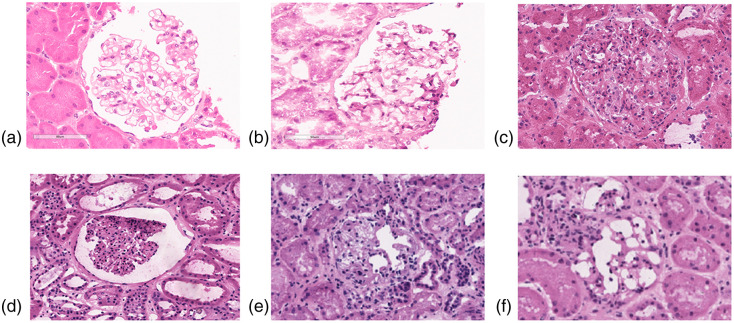
However, DL studies on frozen sections of kidney remain limited.^15,40 Relative to paraffin-embedded tissue, frozen tissue presents a unique challenge in computational renal pathology. For example, glomeruli typically present with better morphology on paraffin-embedded sections versus frozen sections. Furthermore, the variability in stain quality of frozen sections is greater compared with paraffin-embedded sections and depends on multiple variables associated with deceased-donor kidney biopsies (e.g., the underlying illness of the donor, the ischemic time between organ procurement and biopsy, etc.). Other factors that may affect frozen tissue presentation are the room and cryostat temperature where the frozen section was obtained and cut, the humidity of the room that may affect the percentage of water in the staining solution, etc. (Fig. 9).

Fig. 9.

Examples of artifacts in frozen sections compared with paraffin-embedded sections. (a) Example of a glomerulus from a formalin-fixed and paraffin-embedded kidney biopsy stained with H&E (archival image). (b)–(f) Examples of glomeruli from frozen sections stained with H&E: In (b) is represented a glomerulus from a native kidney biopsy that is frozen relatively quickly after the biopsy procedure (archival image), and in (d)–(f) glomeruli from cadaveric donor kidney biopsies that were used in this study. Section folding and freezing artifacts are noted, resulting in high variability in image presentation.

This paper describes the development, characterization, and evaluation of a DL model to automatically detect and segment sclerotic and nonsclerotic glomeruli on frozen sections of donor kidney biopsies prior to organ transplantation. We hypothesized that a DL approach would outperform standard-of-care pretransplant biopsy characterization based on visual glomerular counting. We tested this hypothesis by deploying our proposed model on a multiinstitutional, independent testing dataset, where DL results were compared with historically reported standard-of-care results.

2. Materials and Methods

2.1. Whole Slide Imaging Dataset

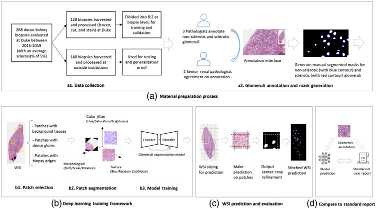
This study was approved by the Duke University Institutional Review Board. A total of 211 kidney donors deceased between January, 2015, and January, 2020, were included in the study, for a total of 268 frozen section H&E-stained slides. Of these, 75 donors had a wedge kidney biopsy performed, frozen, cut, and stained with hematoxylin and eosin (H&E) at Duke University Medical Center (DUMC) for a total of 128 frozen section H&E-stained glass slides (internal cases). Of these 75 donors, 53 had bilateral biopsies and 22 had unilateral biopsies performed. The remaining 136 deceased donors had a wedge kidney biopsy performed, frozen, cut, and stained with H&E in other institutions (external cases) and subsequently reviewed at DUMC, for a total of 140 frozen section H&E-stained slides [Fig. 1(a1)].

Fig. 1.

Overall research design. (a) The material preparation process consisted of collection of cases from DUMC and outside institutions, followed by manual annotation and QC by expert renal pathologists. (b) The training process included selection and augmentation of training samples, followed by model optimization for segmenting the glomeruli. (c) Predictions were made based on sequential patches, which were concatenated together to recover a WSI full field-of-view prediction. (d) The model performance was further investigated by comparing to the standard-of-care report indicating the number of glomeruli based on visual assessment.

Whole slide images (WSIs) were acquired at $40\times$ magnification on a Leica AT2 whole-slide scanner located in the Duke University Department of Pathology’s BioRepository and Precision Pathology Center for all cases. All WSI were reviewed for image quality, where 10 WSIs were excluded because they had with severe artifacts, including excessive folding, poor quality of staining, and the presence of bubbles under the coverslip. Complete exclusion criteria are provided in Table 4. The final WSI dataset included a total of 258 WSIs (123 internal and 135 external).

Table 4.

Slide artifact assessment and quality assurance.

Location of the artifact	Type of artifact	Criteria for discarding WSI by visual assessment	Comment
Glass slide	Dirty glass slide	See comment	Glass slides were cleaned prior to scanning, however occasional glass dust was still present in rare slides prior scanning.
	Pen marking	See comment	Pen marking affected a very small percentage of WSI, and a small fraction of the tissue section, with minimal interference with tissue analysis.
	Cover slip (i.e., cracks)	Broken glass slides were not scanned	n/a
	Mounting medium (i.e., bubble)	Over 50% of the section was compromised	Occasional small bubbles were present in a small fraction of WSI. Those affected the DL performance.
Tissue section	Folding	Over 50% of the section was compromised	Folding of the tissue section is often unavoidable while cutting frozen sections. Those affected the DL performance.
	Knife chatters/holes	Over 50% of the section was compromised	Occasional tissue holes/knife chatters were present in a small fraction of WSI, which affected the DL performance.
	Thickness	Tissue sections were not reliably interpretable by human eye	Variability in tissue thickness was noted.
	Staining	Tissue sections were not reliably interpretable by human eye	Staining variations are very common even within the same laboratory and may affect the performance of the model. However, by using a large dataset for training and validation, we assured a sufficient heterogeneity of staining variation.
	• overstaining
	• understaining
	• uneven staining
	Autolysis	Tissue sections were not reliably interpretable by human eye	Autolysis affects tubules more severely than glomeruli. In glomeruli, autolysis may manifest as more irregular contours of individual glomerular cells (mesangial, endothelial, and visceral and parietal epithelial cells) and structures (mesangium, basement membranes, capsule).
	Freezing procedure	Tissue sections were not reliably interpretable by human eye	Occasional focal freezing artifact present in the tissue can interfere with the model performance.
	Glomerular histologic mimic	N/a	The glomerular histologic mimics represent a learning point for the future to interpret false positive and false negative.
Scanning	Focus	Blurry—out of focus
	Grid noise	No exclusion criteria were defined

2.2. Manual Segmentation of Glomeruli

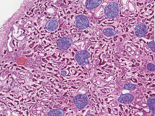
Manual segmentation of glomeruli was performed as follows. Each WSI was first segmented by one of the three junior observers (with 1, 2, and 5 years of experience in pathology). Segmentation was achieved by manually outlining glomeruli in all 258 WSIs using a publicly available digital pathology tool (QuPath, version 0.1.2). For nonsclerotic glomeruli, annotations were made by tracing the Bowman’s capsule and through the vascular and tubular pole of the glomerulus, when visible, to maintain a continuous outline of the individual glomeruli. As the Bowman’s capsule of globally sclerotic glomeruli is generally inconsistent or separated from the tuft by a white space representing a processing/freezing artifact, only the sclerosed tuft was outlined during the segmentation process (Fig. 2).

Fig. 2.

An illustrating example of a WSI with glomerular segmentations. Manual segmentations of nonsclerotic glomeruli (blue segmentations) and sclerotic glomeruli (red segmentations) on WSIs are generated using QuPath.

Following the initial manual segmentation, the dataset was reviewed by two senior renal pathologists with 25 and 40 years of experience in renal pathology, and modifications were made where it was necessary to achieve expert consensus. This procedure was implemented to recapitulate what is clinically done in renal pathology practice (i.e., a trainee performs the first pass of glomeruli counting, which is then reviewed by a senior renal pathologist). Matched pairs of shift-invariant WSIs and manual segmentations were considered as DL training samples [Fig. 1(a2)].

2.3. Deep Learning Implementation and Performance Evaluation

2.3.1. Network architecture

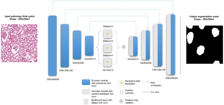
A DL framework was developed to automatically identify and segment nonsclerotic versus globally sclerotic glomeruli on frozen section WSIs. A nine-module convolutional neural network (CNN) based on the common U-Net architecture⁴¹ with a dilated bottleneck was developed for glomerular segmentation (Fig. 3). Our U-Net architecture is a symmetric encoder–decoder fully convolutional network with a $256\times 256\times 3$ input layer that produces pixel-level segmentation results. Each encoder module contains two convolution blocks consisting of a $3\times 3$ convolutional layer, a batch normalization procedure, and a rectified linear unit activation function. Modules are connected by a $2\times 2\max$-pooling layer for downsampling.

Fig. 3.

DL model architecture. (Left) An input glomeruli patch of size $256\times 256\times 3$ is fed into a nine-module U-Net model. For this model, each of the four encoder (i.e., left side of the network) modules are loaded with VGG pretrained weights, which are then finetuned during training. The bottleneck module consists of three dilated convolution layers with different dilation rates. The feature maps at this level are added elementwise at the end of the bottleneck. The four decoder modules (i.e., right side of the network) use transpose convolutions to upsample the feature maps, and skip-connections incorporate the encoder information. Finally, a $1\times 1$ convolution layer maps the information to a $256\times 256$ binary image of pixel-level predictions of glomerular locations.

The downsampled bottleneck module consists of three dilation operations⁴² for each convolutional layer, which enlarge the receptive field to capture coarse field-of-view imaging details within the high-level feature maps. The decoder modules recover and upsample the semantic information generated from the bottleneck module, each of which includes a $2\times 2$ transpose convolution block and a $3\times 3$ convolution block. Long-term skip connections are used for enhancing different scale texture details provided in the encoding layers. Finally, a $1\times 1$ convolutional layer is used to output a two-layer probability map representing glomerular foreground versus background.

2.3.2. Model training and validation

The 75 internal cases (123 WSIs) were divided at the patient level into training and validation datasets with a 0.8:0.2 ratio, respectively, and used to train/fine-tune the DL model. The 135 external cases (135 WSIs) were used as an independent testing dataset. The training dataset consisted of tissue that was cut and stained at Duke University under a standard institutional protocol used for clinical practice. As testing data were—by design—acquired from other institutions, there was a higher variation in tissue sectioning and staining protocols. The rationale for this experimental design was to provide a good estimate of true model generalization when applied to heterogeneous data.

Two independent models were trained in parallel for normal and globally sclerotic glomeruli, respectively. A well-balanced, patch-based training set that represented both glomerular signal and background tissue was engineered as follows. Each WSI of the training set was stochastically sampled with 500 iterations by extracting random $256\times 256$ patches from the entire tissue field-of-view. Patches with a glomerular pixel density of at least 20% were included as training examples (i.e., to represent a high degree of glomerular signal during the training process). Patches with a glomerular pixel density of 0% (i.e., no glomeruli in the patch) were also included as training examples (i.e., to represent pure background tissue during the training process). Patches with a nonzero glomerular pixel density $<20\%$ were excluded from the training dataset to minimize partial volume effects and edges of different glomeruli at the perimeter of the patch. Matched pairs of shift-invariant image patches and corresponding manual segmentations were used as training examples.

To boost model generalization, a data augmentation procedure was applied, including basic operations (e.g., horizontal vertical flip, crop resize), morphological transformations (e.g., shift scale rotate, elastic transform), color distortions (e.g., contrast brightness, hue saturation value), and other image processing operations (Gaussian blur, random cutout). Training also utilized transfer learning, where the network’s first four fully convolutional blocks were initialized as the pretrained ImageNet⁴³ weights of the publicly available VGG16²⁸ data. During the training process, a cross entropy loss function was minimized based on Adam optimization³⁷ to learn optimal model hyperparameterization. Training was run for 200 epochs with a batch size of 16 input patches and an initial learning rate of 0.001. The training implementation achieving the lowest validation loss was computationally locked down and deployed as the final model for testing.

2.3.3. Model testing

Model performance was independently evaluated on the testing dataset. Each testing set WSI was decomposed into nonoverlapping patches using a sliding window technique, and the model was applied in a patch-by-patch basis and then concatenated together to generate a biopsy-level prediction at the full $40\times$ field-of-view. Glomeruli at the perimeter of patches were handled with a patch padding technique, where the model was applied to 50% padded windows and then cropped to the original patch size. This was done to avoid clipping artifacts of glomeruli at the border of each patch.

Since our testing dataset consisted of multi-institutional data, there was variation in color distribution compared with the training dataset. As such, a stain color normalization method⁴⁴ was performed to match the color density of each testing image to a uniform reference color space, while preserving histology structure.

Segmentation accuracy was quantified based on the dice similarity coefficient (DSC),⁴⁵ which measures the pixel-level overlap between DL-generated segmentation results and manual segmentation results. In addition, model accuracy, sensitivity, and specificity of sclerotic versus nonsclerotic glomeruli were quantified based on $F1$, precision, and recall scores.⁴⁶

2.3.4. Effect of transfer learning and color variation on model performance

The effect of transfer learning and sample size on model performance was evaluated for both nonsclerotic and sclerotic glomeruli segmentation models. Model performance metrics with and without the transferred VGG16 weights were compared and their differences quantified. To evaluate the effect of color variation, model performance was compared with and without test-time color normalization.

2.4. Deep Learning Glomerular Count versus Standard of Care Pathology Reporting

External cases where the reported glomerular count was available ($N=47$) were used to compare the DL-derived glomerular count to the current standard of care. The reported glomerular counts for nonsclerotic and globally sclerotic glomeruli performed on the frozen section, along with the sclerotic-nonsclerotic glomerular ratio, were compared with both the corresponding manual segmentation-derived counts and the DL-derived counts [Fig. 1(d)].

Pairwise $t$-tests and Pearson correlation coefficients were used to quantify statistical differences between the (a) historically reported, (b) manual segmentation-derived, and (c) DL-derived glomerular count. The Bonferroni–Holm method⁴⁷ was implemented to correct $p$-values for multiple hypotheses testing. A corrected $p$-value lower than 0.05 was considered statistically significant.

3. Results

3.1. Manual Segmentation of Glomeruli

A total of 21,146 nonsclerotic (8897 from the internal dataset and 12,249 from the external dataset) and 1322 sclerotic glomeruli (682 from the internal dataset and 640 from the external dataset) were manually segmented on 258 images.

3.2. Deep Learning Detection and Segmentation Performance

DL model performance results on the external testing WSIs are summarized in Table 1. The nonsclerotic glomeruli model achieved a DSC of 0.91 (implying high spatial overlap compared to manual segmentation), an $F1$ score of 0.93 (implying strong overall detection performance), high recall of 0.96 (implying accurate recognition of true positive nonsclerotic glomeruli), and high precision of 0.90 (indicating a high overprediction of nonsclerotic glomeruli compared to sclerotic glomeruli). Similarly, the sclerotic glomeruli model achieved a DSC of 0.83, an $F1$ score of 0.87, recall of 0.93, and a precision of 0.81. A WSI final prediction example is visualized in Fig. 4.

Table 1.

Model performance on the testing dataset. Glomerular detection and segmentation performance for the nonsclerotic glomeruli were $>0.9$ for all performance metrics. The sclerotic performance was slightly less robust but still good with measures $>0.8$ with recall being 0.91. The slightly worse precision compared to recall means there were more false positives than false negatives. When compared with the performance of the nonsclerotic algorithm, the precision is less robust which is consistent with the smaller amount of data in the sclerotic cohort and the relatively greater variety histologic mimics of sclerotic glomeruli on the WSIs.

	Detection			Segmentation
	Precision	Recall	$F1$	DSC
Nonsclerotic	0.898	0.957	0.926	0.901
Sclerotic	0.812	0.931	0.865	0.829

Fig. 4.

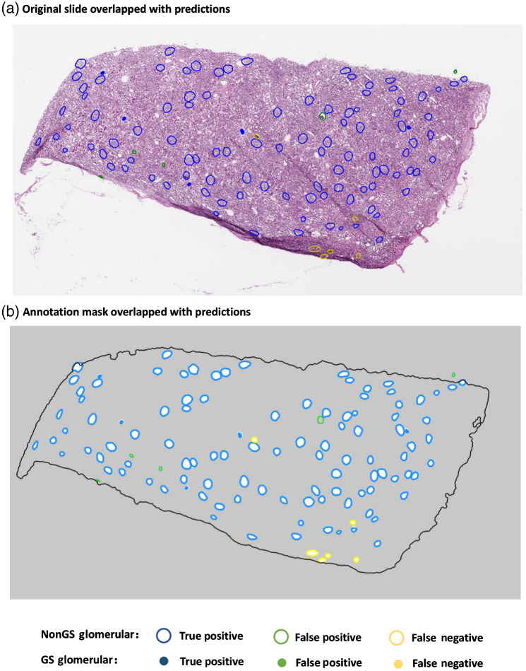
An illustrating example (testing set) of DL segmentation of glomeruli on a WSI. Results are color coded relative to reference manual annotations to demonstrate the performance of the DL algorithm on testing data.

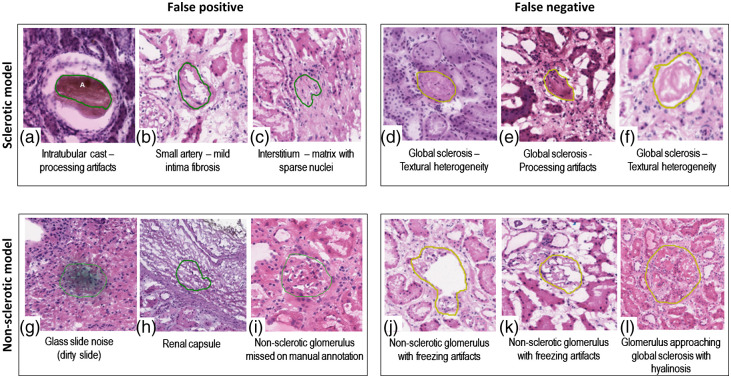
Figure 5 shows examples of false-positive and false-negative predictions of sclerotic and nonsclerotic models. Sources of model error included two major categories: procedure artifacts (e.g., tissue processing artifacts such as overstaining, folds, air bubbles, and chatter) and glomerular histologic mimics (e.g., fibrosis of the urinary space, dense interstitial fibrosis, and red blood cell casts). The global sclerosis model had a relatively high false positive rate, due to the variety of sclerotic textures and the relative lack of global sclerosis training data. Hence, most of the incorrect predictions were due to histology mimics. The nonsclerotic model generally learned well. Extreme procedure artifacts (e.g., distorted glomeruli, tangential cuts with small glomerular profiles, and poor staining) were the major reasons for failed predictions.

Fig. 5.

False-positive and false-negative predictions for globally sclerotic and nonsclerotic glomeruli. (a)–(c) False positive for the global sclerosis model; (d)–(f) false negative for the global sclerosis model; (g)–(i) false positive for the nonglobal sclerosis model. (i) A probable nonglobally sclerotic glomerulus was not manually annotated by the primary annotator nor by the quality control pathologist, but it was detected by the DL model; (j)–(l) false negative for the nonglobal sclerosis model.

3.3. Effect of Transfer Learning and Color Normalization on Model Performance

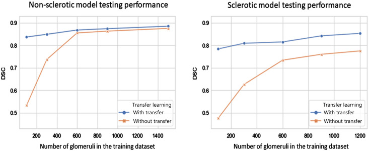
As shown in Fig. 6, when training on a relatively small sample size (e.g., number of glomeruli $<600$), transfer learning had a significant effect on DL model performance. Despite less data, model performance was improved based on the transfer learning procedure. The effect of transfer learning was less significant when $>600$ glomeruli were used for training. The nonsclerotic glomeruli model required less training samples (i.e., 1500 nonsclerotic glomeruli) to achieve performance saturation (i.e., $\mathrm{DSC}=0.9$) compared with the sclerotic glomeruli model. Meanwhile, the sclerotic glomeruli model appeared to not achieve performance saturation, implying that more sclerotic data would likely improve performance. As demonstrated in Table 2, test-time color normalization had a nominal effect on model performance, which shows the DL training pipeline with suitable data augmentation can help resist color variation in the data source.

Fig. 6.

Effect of transfer learning and sample size on model performance of (left) nonsclerotic glomeruli and (right) sclerotic glomeruli. Transfer learning improved model performance significantly with limited data (i.e., $<600$ glomeruli) for both (a) nonsclerotic and (b) sclerotic model. Less glomeruli samples are needed for the nonsclerotic model to reach a performance saturation (i.e., $\mathrm{DSC}=0.9$ with 1500 glomeruli), compared to sclerotic model.

Table 2.

Effect of test-time color normalization on model performance.

	Detection			Segmentation
	Precision	Recall	$F1$	DSC
Noncolor normalized
Nonsclerotic	0.898	0.957	0.926	0.901
Sclerotic	0.812	0.931	0.865	0.829
Color normalized
Nonsclerotic	0.908	0.963	0.934	0.907
Sclerotic	0.807	0.934	0.863	0.824

3.4. Deep Learning Glomerular Count versus Standard of Care Pathology Reporting

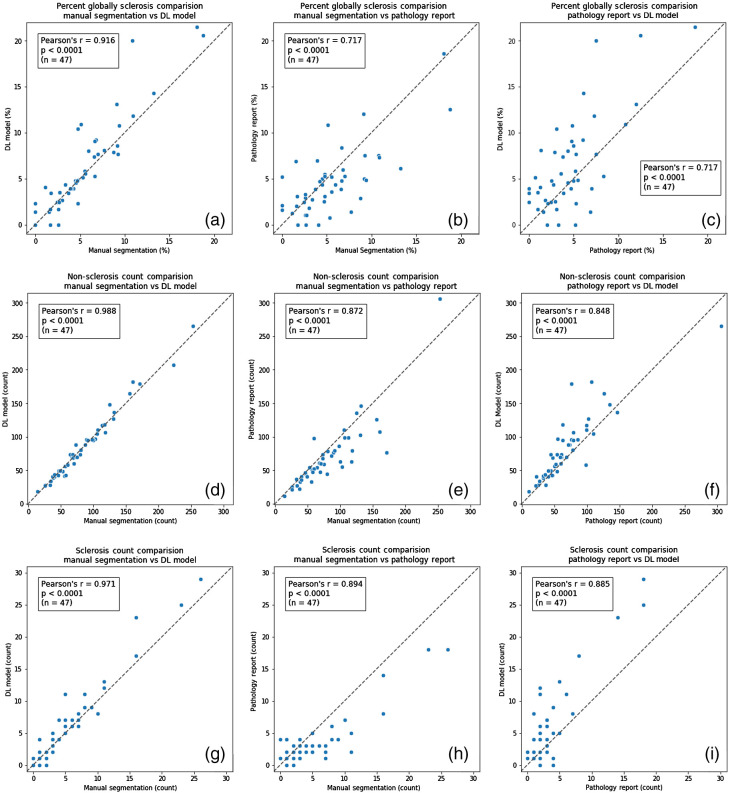
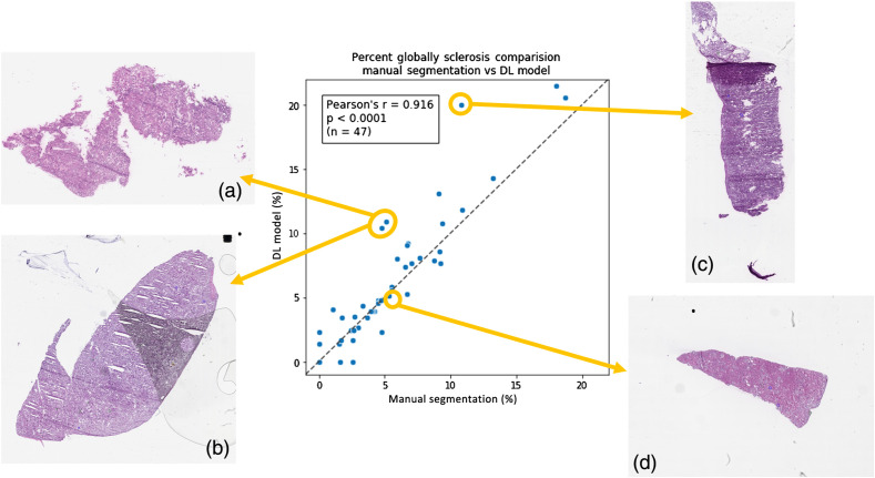
Direct statistical comparisons between (i) historically reported glomerular counts, (ii) manual segmentation glomerular counts, and (iii) DL-model glomerular counts are reported in Table 3. When the glomerular count from the manual segmentation was compared with the glomerular count from the DL model, statistically similar counts were observed for both nonsclerotic ($p=0.837$) and sclerotic glomeruli ($p=0.0950$). This implies that the DL-model is operating at a noninferior counting performance relative to an expert renal pathologist. When the glomerular counts from the manual and DL segmentation were compared to the historically reported standard-of-care glomerular counts, a statistically significant difference was observed for both nonsclerotic ($p=<0.0001$) and sclerotic ($p=0.002$) glomeruli. This implies that both manual counting by a renal pathologist and automatic counting by the DL model are both more accurate than historically reported clinical data. Correlation plots of the three category results among three methods for each data point are shown in Fig. 7. In Fig. 8, testing WSIs on the correlation plot are displayed with different procedure artifact conditions, which were a major source of model performance deviation.

Table 3.

Comparison of glomerular counts. For the non-sclerotic model, the model-annotation count is not significantly different from the reference segmentations, whereas the standard of care count is different from the reference segmentations. The same is true for the sclerotic model, which is not significantly different from the reference segmentations, whereas the standard of care has a significantly different count from the reference segmentations.

	Manual segmentation	DL model	Pathology report	Manual segmentation versus DL model	Manual segmentation versus pathology report	DL model versus pathology report
	Average number (range)	Average number (range)	Average number (range)
Nonsclerotic	84.6 ± 14.5 (14 to 253)	85.0 ± 15.2 (18 to 265)	75.6 ± 18.3 (11 to 306)	p = 0.837	p = 1.3426e-6	p = 1.085e-7
Sclerotic	5.3 ± 1.7 (0 to 26)	6.0 ± 1.9 (0 to 29)	3.4 ± 1.2 (0 to 18)	p = 0.095	p = 0.002	p = 0.002
% Sclerosis	5.5 ± 1.2 (0 to 18.75)	6.4 ± 1.5 (0 to 21.48)	4.6 ± 1.1 (0 to 18.56)	p = 0.385	p = 0.256	p = 0.060

Fig. 7.

Glomerular characterization results on testing data samples for the DL model, manual segmentation, and standard-of-care pathology reporting. High Pearson correlation demonstrates good agreement between DL and manual segmentation, relative to standard-of-care pathology reporting results. (a)–(c) The percentage of sclerotic glomeruli detected by the DL model compared to the pathology report and the manual segmentations. (d)–(f) The absolute number of nonsclerotic glomeruli detected by the DL model compared to the pathology report and the manual segmentations. (g)–(i) The absolute number of sclerotic glomeruli detected by the DL model compared to the pathology report and the manual segmentations. These findings indicate that DL-based glomerular characterization outperforms historical pathology reporting results based on standard-of-care methods.

Fig. 8.

Visualization of WSIs relative to model performance on testing data. (a)–(c) WSIs contain tissue freezing and folding artifacts, glass slide (bubble between the cover slip and the glass slide) and cutting artifacts, and tissue folding artifacts, which may have contributed to decreased performance. (d) The tissue section is intact and without artifacts, with accuracy for sclerosis from the DL model prediction.

4. Discussion

Digital pathology and state-of-the-art computational techniques are changing the landscape of pathology practice.²⁴ Unlike in oncologic pathology, where computational image analysis has been extensively developed and is slowly being introduced into clinical practice, drug development, and clinical trials,⁴⁸ native and transplant nephropathology still relies entirely on visual assessment. In the current study, we developed a robust, accurate, and generalizable DL model for automatic segmentation of nonsclerotic and globally sclerotic glomeruli on H&E frozen section WSIs from donor kidney wedge biopsies. Compared to paraffin-embedded sections, glomeruli on frozen tissue have inferior morphology and more artifacts. Illustrating examples are included in Fig. 9. We stress that interrogation of frozen tissue is paramount to clinical transplant medicine. Our results demonstrate high predictive performance on an independent dataset and show that machine-derived glomerular counts are more accurate than historically reported standard-of-care clinical data. These positive findings provide hypothesis generating data and motivate future applications of AI techniques to transplant medicine.

While other groups have primarily investigated DL-based glomerular detection and segmentation on WSIs of paraffin-embedded tissue,^{38–40,49–62} our study represents the largest application using frozen sections from kidney donor wedge biopsies. Previous work by Marsh et al. successfully demonstrated elliptical detection¹⁵ and quantification⁴⁰ of glomeruli on frozen sections. Although their approach to DL was different than ours and their cross-validated model lacked independent testing, our key findings are comparable and thus both provide promising insight.

The generalization of DL models is critical for future clinical translation. Even though laboratories in the United States follow general College of American Pathology (CAP)^21,26 and Clinical Laboratory Improvement Amendments (CLIA) guidelines,⁶³ pre-analytical variability is still significant. Computational pathology techniques are highly sensitive to pre-analytical tissue variations²⁴ (Fig. 9), including room and freezing temperature, wedge biopsy tissue thickness, the percentage of water in the biopsy tissue (freezing artifacts), frozen section thickness, the presence of folds (cutting artifacts), and composition of the stain solutions (stain artifacts).²⁷ These tissue artifacts are summarized in the appendix under Table 4. Furthermore, the time from organ procurement from the deceased donor to biopsy/implantation (ischemic time) is often highly variable (sometimes in excess of 24 hours). Longer time delays from death to implantation often lead to greater autolysis artifacts on the frozen sections. Pre-existing conditions leading to patient death can also degrade tissue presentation, although these generally affect tubules and interstitium more so than glomeruli. Unlike the previously published work,^15,40 our model was independently evaluated on a multi-institutional test dataset. Thus, our results provide a reasonable representation of how well the model generalized to new information not observed during training. Since independent model testing is a hallmark of quality machine learning, this is a key novelty of our research design.

Our data have also shown that the DL algorithm on digital images operates with more accuracy than clinical reads using conventional microscopy. Several reasons may account for this increased performance. First, often, pathologists assessing frozen sections donor biopsies not only operate overnight but also are not subspecialty trained in renal pathology. Second, the spatial–visual memory of any human is limited, resulting in missing some glomeruli while counting or counting the same glomeruli twice. The manual annotation of all the glomeruli allows for the mapping of the glomeruli on the WSIs, so the count can be more accurate⁵¹ and serve as a better clinical marker.

In this work, we chose to implement a UNET architecture that incorporated several state-of-the-art techniques, including transfer learning, data augmentation, and convolutional dilation.⁶⁴ The motivation behind this design choice was based on recently published work, where UNET was successfully implemented to segment glomeruli on nonfrozen tissue.^38,65,66 Since our work is the first of its kind on frozen tissue, we chose a relatively simple model architecture that is commonly used in diverse biomedical image segmentation applications. We acknowledge, however, that there are newer DL architectures, some of which have been applied to glomeruli detection, including the Inception V3 Architecture.⁶⁷ Future work will focus on comparing different model architectures on frozen tissue, including advanced segmentation networks, such as DeepLab V3⁴² and Mask R-CNN,⁶⁸ and effective network modules, such as residual blocks⁶⁹ and attention blocks.⁷⁰ While such an analysis is out of scope of the current work, the characterization of different model architectures is essential to eventually implementing these new technologies in clinical practice.

We note that many classical algorithms do very well at glomeruli detection, including multiradial local binary patterns,⁴⁹ HOG descriptors,⁵³ and Butterworth band-pass filtering.⁷¹ However, these techniques often require multimodal imaging, do not generalize well to glomerular segmentation, or result in highly polygonal approximations of Bowman’s space. While the detection of glomeruli is important to pretransplant clinical workup, segmentation is essential to more sophisticated downstream glomerular characterization and new biomarker discovery. Thus, our goal was to develop a workflow to perform both detection of glomeruli (to recapitulate standard-of-care clinical practice) and segmentation of glomeruli (to promote next-generation characterization of glomeruli via pathomic feature extraction).

Nevertheless, we believe our research design is suitable for the current dataset. First, transfer learning was shown to boost model performance using pretrained weights obtained from the publicly available ImageNet database as initial parameter conditions.⁷² This implies that these natural images encode generalized features of quantitative image representation that are applicable to digital pathology tasks. Our results demonstrate that the relative effect of transfer learning is indirectly proportional to sample size. This finding is consistent with machine learning theory^73,74 and implies that the performance of our sclerotic glomeruli model may asymptotically improve with more data. Second, data augmentation was also shown to increase the generalization of our DL results, suggesting artificial augmentations may capture important characteristics of renal pathology.²⁵ For example, shape deformation was shown to be effective in improving the recognition of various shapes and sizes of glomeruli. In addition, color jitter was useful to harmonize the large variation in stain quality, especially between the training data and the testing data. We observed sclerotic glomeruli to be most affected by color jitter, whereas nonsclerotic glomeruli were more sensitive to texture deformation. We hypothesize that this is due to sparser image texture in the compact structure of sclerotic glomeruli. Other augmentation methods (e.g., Gaussian blur) generally yielded better performance in the presence of freezing artifacts. Finally, our network architecture included a dilated block at the bottleneck.^{25,69,70,72–74} The rationale behind this design choice was to enable a larger receptive field-of-view to aggregate multiscale imaging information. Based on our results, we found that this dilation procedure reduced misclassification errors in the presence of tissue fold artifacts.

While our results are promising, this study has some limitations. First, all images were acquired on the same whole slide scanner. As such, it is currently unclear how scanning variability will affect the quality and performance of our trained DL models. Future work should address these issues based on dedicated quality assurance software for digital pathology⁷⁵ and digital phantoms as reference, which is becoming common practice in quantitative radiology applications.^76,77 Second, differences in model performance noted between the nonsclerotic and globally sclerotic glomeruli were due to the limited number of globally sclerotic glomeruli in the WSI dataset. We anticipate that model performance will increase based on more examples of sclerotic glomeruli. Finally, while our approach generated a robust reference segmentation dataset reflecting institutional renal pathology practice, interobserver variability was not addressed in this work. To minimize interobserver variability, future work should focus on using immunofluorescent and/or immunohistochemical stains that are shift-invariant to H&E images⁷¹ or conduct observer studies to generate robust reference datasets.

In conclusion, the work developed, characterized, and evaluated a DL model to automatically detect and segment sclerotic and nonsclerotic glomeruli on frozen sections of donor kidney biopsies prior to organ transplantation. Digital pathology and automatic image analysis enable solutions that may aid in the clinical transplant nephropathology environment by providing robust and standardized quantitative observations, higher efficiency, centralized interpretation by expert pathologists with overall reduced error rates,⁷⁸ and by reducing the known limitations associated with visual examination.^14,16,24 In addition, a digital solution offers a more rapid and efficient allocation of the kidney overcoming the limitations, expenses, and loss of precious time from the transferring of a donor organ and associated frozen section of the wedge biopsy from institution to institution, in search of a recipient.

Biographies

Xiang Li is a PhD student in electrical and computer engineering in the Latafa Lab. She received her BS degree in communication engineering from Northwest University in China and her MS degree in electrical and computer engineering from Duke University. Her research interests are medical image analysis, digital pathology, computer vision, and deep learning.

Kyle J. Lafata is an assistant professor of radiology, radiation oncology, and electrical and computer engineering at Duke University. He received his PhD in medical physics from Duke University and completed postdoctoral training at the U.S. Department of Veterans Affairs in the Big Data Scientist Training Enhancement Program. The Lafata Lab focuses on the theory, development, and application of multiscale imaging biomarkers.

Laura Barisoni is a professor of pathology and medicine, director of the Renal Pathology Service, and co-director of the Division of AI and Computational Pathology at Duke University. She is a co-investigator in several consortia to study kidney diseases. Her main focus of interest is digital pathology and the development and application of tools for the detection and classification of histologic primitives, and the extraction of information for prognostication and prediction of kidney disease outcomes.

Biographies of the other authors are not available.

Disclosures

The authors have no conflict of interests to disclose.

Code, Data, and Materials Availability

The raw data and model source code for this study can be obtained through correspondence with the corresponding authors.

References

- 1.Wolfe R. A., et al. , “Comparison of mortality in all patients on dialysis, patients on dialysis awaiting transplantation, and recipients of a first cadaveric transplant,” N. Engl. J. Med. 341(23), 1725–1730 (1999). 10.1056/NEJM199912023412303 [DOI] [PubMed] [Google Scholar]
- 2.Plage H., et al. , “Extended criteria donors in living kidney transplantation including donor age, smoking, hypertension and BMI,” Ther. Clin. Risk Manage. 16, 787–793 (2020). 10.2147/TCRM.S256962 [DOI] [PMC free article] [PubMed] [Google Scholar]
- 3.Hart A., et al. , “OPTN/SRTR 2018 annual data report: kidney,” Am. J. Transpl. 20(Suppl. s1), 20–130 (2020). 10.1111/ajt.15672 [DOI] [PubMed] [Google Scholar]
- 4.Angeletti A., Cravedi P., “Making procurement biopsies important again for kidney transplant allocation,” Nephron 142(1), 34–39 (2019). 10.1159/000499452 [DOI] [PubMed] [Google Scholar]
- 5.Kasiske B. L., et al. , “The role of procurement biopsies in acceptance decisions for kidneys retrieved for transplant,” Clin. J. Am. Soc. Nephrol. 9(3), 562–571 (2014). 10.2215/CJN.07610713 [DOI] [PMC free article] [PubMed] [Google Scholar]
- 6.Dahmen M., et al. , “Validation of the kidney donor profile index (KDPI) to assess a deceased donor’s kidneys’ outcome in a European cohort,” Sci. Rep. 9(1), 11234 (2019). 10.1038/s41598-019-47772-7 [DOI] [PMC free article] [PubMed] [Google Scholar]
- 7.Carpenter D., et al. , “Procurement biopsies in the evaluation of deceased donor kidneys,” Clin. J. Am. Soc. Nephrol. 13(12), 1876–1885 (2018). 10.2215/CJN.04150418 [DOI] [PMC free article] [PubMed] [Google Scholar]
- 8.Teixeira A. C., et al. , “Evaluation of frozen and paraffin sections using the Maryland aggregate pathology index score in donor kidney biopsy specimens of a Brazilian cohort,” Transpl. Proc. 49(10), 2247–2250 (2017). 10.1016/j.transproceed.2017.11.004 [DOI] [PubMed] [Google Scholar]
- 9.Sagasta A., et al. , “Pre-implantation analysis of kidney biopsies from expanded criteria donors: testing the accuracy of frozen section technique and the adequacy of their assessment by on-call pathologists,” Transpl. Int. 29, 234–240 (2016). 10.1111/tri.12709 [DOI] [PubMed] [Google Scholar]
- 10.El-Husseini A., et al. , “Can donor implantation renal biopsy predict long-term renal allograft outcome?” Am. J. Nephrol. 27(2), 144–151 (2007). 10.1159/000099944 [DOI] [PubMed] [Google Scholar]
- 11.Salvadori M., Tsalouchos A., “Histological and clinical evaluation of marginal donor kidneys before transplantation: which is best?” World J. Transpl. 9(4), 62–80 (2019). 10.5500/wjt.v9.i4.62 [DOI] [PMC free article] [PubMed] [Google Scholar]
- 12.Goumenos D. S., et al. , “The prognostic value of frozen section preimplantation graft biopsy in the outcome of renal transplantation,” Ren. Fail 32(4), 434–439 (2010). 10.3109/08860221003658241 [DOI] [PubMed] [Google Scholar]
- 13.Munivenkatappa R. B., et al. , “The Maryland aggregate pathology index: a deceased donor kidney biopsy scoring system for predicting graft failure,” Am. J. Transpl. 8(11), 2316–2324 (2008). 10.1111/j.1600-6143.2008.02370.x [DOI] [PubMed] [Google Scholar]
- 14.Liapis H., et al. , “Banff histopathological consensus criteria for preimplantation kidney biopsies,” Am. J. Transpl. 17(1), 140–150 (2017). 10.1111/ajt.13929 [DOI] [PMC free article] [PubMed] [Google Scholar]
- 15.Marsh J. N., et al. , “Deep learning global glomerulosclerosis in transplant kidney frozen sections,” IEEE Trans. Med. Imaging 37(12), 2718–2728 (2018). 10.1109/TMI.2018.2851150 [DOI] [PMC free article] [PubMed] [Google Scholar]
- 16.Azancot M. A., et al. , “The reproducibility and predictive value on outcome of renal biopsies from expanded criteria donors,” Kidney Int. 85(5), 1161–1168 (2014). 10.1038/ki.2013.461 [DOI] [PubMed] [Google Scholar]
- 17.Roufosse C., et al. , “A 2018 reference guide to the Banff classification of renal allograft pathology,” Transplantation 102(11), 1795–1814 (2018). 10.1097/TP.0000000000002366 [DOI] [PMC free article] [PubMed] [Google Scholar]
- 18.Loupy A., et al. , “Prediction system for risk of allograft loss in patients receiving kidney transplants: international derivation and validation study,” BMJ 366, l4923 (2019). 10.1136/bmj.l4923 [DOI] [PMC free article] [PubMed] [Google Scholar]
- 19.Pantanowitz L., et al. , “Twenty years of digital pathology: an overview of the road travelled, what is on the horizon, and the emergence of vendor-neutral archives,” J. Pathol. Inf. 9, 40 (2018). 10.4103/jpi.jpi_69_18 [DOI] [PMC free article] [PubMed] [Google Scholar]
- 20.Retamero J. A., Aneiros-Fernandez J., Del Moral R. G., “Complete digital pathology for routine histopathology diagnosis in a multicenter hospital network,” Arch. Pathol. Lab. Med. 144(2), 221–228 (2020). 10.5858/arpa.2018-0541-OA [DOI] [PubMed] [Google Scholar]
- 21.Pantanowitz L., et al. , “Validating whole slide imaging for diagnostic purposes in pathology: guideline from the College of American Pathologists Pathology and Laboratory Quality Center,” Arch. Pathol. Lab. Med. 137(12), 1710–1722 (2013). 10.5858/arpa.2013-0093-CP [DOI] [PMC free article] [PubMed] [Google Scholar]
- 22.Brachtel E., Yagi Y., “Digital imaging in pathology—current applications and challenges,” J. Biophotonics 5(4), 327–335 (2012). 10.1002/jbio.201100103 [DOI] [PubMed] [Google Scholar]
- 23.Baidoshvili A., et al. , “Evaluating the benefits of digital pathology implementation: time savings in laboratory logistics,” Histopathology 73(5), 784–794 (2018). 10.1111/his.13691 [DOI] [PubMed] [Google Scholar]
- 24.Barisoni L., et al. , “Digital pathology and computational image analysis in nephropathology,” Nat. Rev. Nephrol. 16(11), 669–685 (2020). 10.1038/s41581-020-0321-6 [DOI] [PMC free article] [PubMed] [Google Scholar]
- 25.Tellez D., et al. , “Quantifying the effects of data augmentation and stain color normalization in convolutional neural networks for computational pathology,” Med. Image Anal. 58, 101544 (2019). 10.1016/j.media.2019.101544 [DOI] [PubMed] [Google Scholar]
- 26.Evans A. J., et al. , “US Food and Drug Administration approval of whole slide imaging for primary diagnosis: a key milestone is reached and new questions are raised,” Arch. Pathol. Lab. Med. 142(11), 1383–1387 (2018). 10.5858/arpa.2017-0496-CP [DOI] [PubMed] [Google Scholar]
- 27.Bauer T. W., et al. , “Validation of whole slide imaging for frozen section diagnosis in surgical pathology,” J. Pathol. Inf. 6, 49 (2015). 10.4103/2153-3539.163988 [DOI] [PMC free article] [PubMed] [Google Scholar]
- 28.Simonyan K., Zisserman A., “Very deep convolutional networks for large-scale image recognition,” arXiv:1409.1556 (2014).
- 29.Abels E., et al. , “Computational pathology definitions, best practices, and recommendations for regulatory guidance: a white paper from the Digital Pathology Association,” J. Pathol. 249(3), 286–294 (2019). 10.1002/path.5331 [DOI] [PMC free article] [PubMed] [Google Scholar]
- 30.LeCun Y., Bengio Y., Hinton G., “Deep learning,” Nature 521(7553), 436–444 (2015). 10.1038/nature14539 [DOI] [PubMed] [Google Scholar]
- 31.Janowczyk A., Madabhushi A., “Deep learning for digital pathology image analysis: a comprehensive tutorial with selected use cases,” J. Pathol. Inf. 7, 29 (2016). 10.4103/2153-3539.186902 [DOI] [PMC free article] [PubMed] [Google Scholar]
- 32.Litjens G., et al. , “A survey on deep learning in medical image analysis,” Med. Image Anal. 42, 60–88 (2017). 10.1016/j.media.2017.07.005 [DOI] [PubMed] [Google Scholar]
- 33.Madabhushi A., Lee G., “Image analysis and machine learning in digital pathology: challenges and opportunities,” Med. Image Anal. 33, 170–175 (2016). 10.1016/j.media.2016.06.037 [DOI] [PMC free article] [PubMed] [Google Scholar]
- 34.Wang S., et al. , “Pathology image analysis using segmentation deep learning algorithms,” Am. J. Pathol. 189(9), 1686–1698 (2019). 10.1016/j.ajpath.2019.05.007 [DOI] [PMC free article] [PubMed] [Google Scholar]
- 35.Bejnordi B. E., et al. , “Diagnostic assessment of deep learning algorithms for detection of lymph node metastases in women with breast cancer,” JAMA 318(22), 2199–2210 (2017). 10.1001/jama.2017.14585 [DOI] [PMC free article] [PubMed] [Google Scholar]
- 36.Ertosun M. G., Rubin D. L., “Automated grading of gliomas using deep learning in digital pathology images: a modular approach with ensemble of convolutional neural networks,” AMIA Annu. Symp. Proc. 2015, 1899–908 (2015). [PMC free article] [PubMed] [Google Scholar]
- 37.Kingma D. P., Ba J., “Adam: a method for stochastic optimization,” arXiv:1412.6980 (2014).
- 38.Jayapandian C. P., et al. , “Development and evaluation of deep learning-based segmentation of histologic structures in the kidney cortex with multiple histologic stains,” Kidney Int. 99(1), 86–101 (2021). 10.1016/j.kint.2020.07.044 [DOI] [PMC free article] [PubMed] [Google Scholar]
- 39.Bukowy J. D., et al. , “Region-based convolutional neural nets for localization of Glomeruli in trichrome-stained whole kidney sections,” J. Am. Soc. Nephrol. 29(8), 2081–2088 (2018). 10.1681/ASN.2017111210 [DOI] [PMC free article] [PubMed] [Google Scholar]
- 40.Marsh J. N., et al. , “Development and validation of a deep learning model to quantify glomerulosclerosis in kidney biopsy specimens,” JAMA Network Open 4, e2030939 (2021). 10.1001/jamanetworkopen.2020.30939 [DOI] [PMC free article] [PubMed] [Google Scholar]
- 41.Ronneberger O., Fischer P., Brox T., “U-Net: convolutional networks for biomedical image segmentation,” arXiv:1505.04597 (2015).
- 42.Chen L.-C., et al. , “DeepLab: semantic image segmentation with deep convolutional nets, atrous convolution, and fully connected CRFs,” arXiv:1606.00915 (2016). [DOI] [PubMed]
- 43.Russakovsky O., et al. , “ImageNet large scale visual recognition challenge,” arXiv:1409.0575 (2014).
- 44.Vahadane A., et al. , “Structure-preserving color normalization and sparse stain separation for histological images,” IEEE Trans. Med. Imaging 35(8), 1962–1971 (2016). 10.1109/TMI.2016.2529665 [DOI] [PubMed] [Google Scholar]
- 45.Zou K. H., et al. , “Statistical validation of image segmentation quality based on a spatial overlap index,” Acad. Radiol. 11(2), 178–189 (2004). 10.1016/S1076-6332(03)00671-8 [DOI] [PMC free article] [PubMed] [Google Scholar]
- 46.Sokolova M., Lapalme G., “A systematic analysis of performance measures for classification tasks,” Inf. Process. Manag. 45, 427–437 (2009). 10.1016/j.ipm.2009.03.002 [DOI] [Google Scholar]
- 47.Aickin M., Gensler H., “Adjusting for multiple testing when reporting research results: the Bonferroni vs. Holm methods,” Am. J. Public Health 86(5), 726–728 (1996). 10.2105/AJPH.86.5.726 [DOI] [PMC free article] [PubMed] [Google Scholar]
- 48.Bera K., et al. , “Artificial intelligence in digital pathology – new tools for diagnosis and precision oncology,” Nat. Rev. Clin. Oncol. 16(11), 703–715 (2019). 10.1038/s41571-019-0252-y [DOI] [PMC free article] [PubMed] [Google Scholar]
- 49.Simon O., et al. , “Multi-radial LBP features as a tool for rapid glomerular detection and assessment in whole slide histopathology images,” Sci. Rep. 8, 2032 (2018). 10.1038/s41598-018-20453-7 [DOI] [PMC free article] [PubMed] [Google Scholar]
- 50.Kannan S., et al. , “Segmentation of glomeruli within trichrome images using deep learning,” Kidney Int. Rep. 4(7), 955–962 (2019). 10.1016/j.ekir.2019.04.008 [DOI] [PMC free article] [PubMed] [Google Scholar]
- 51.Rosenberg A. Z., et al. , “The application of digital pathology to improve accuracy in glomerular enumeration in renal biopsies,” PLoS One 11(6), e0156441 (2016). 10.1371/journal.pone.0156441 [DOI] [PMC free article] [PubMed] [Google Scholar]
- 52.Gadermayr M., et al. , “Generative adversarial networks for facilitating stain-independent supervised and unsupervised segmentation: a study on kidney histology,” IEEE Trans. Med. Imaging 38(10), 2293–2302 (2019). 10.1109/TMI.2019.2899364 [DOI] [PubMed] [Google Scholar]
- 53.Kato T., et al. , “Segmental HOG: new descriptor for glomerulus detection in kidney microscopy image,” BMC Bioinf. 16, 316 (2015). 10.1186/s12859-015-0739-1 [DOI] [PMC free article] [PubMed] [Google Scholar]
- 54.Gadermayr M., et al. , “CNN cascades for segmenting sparse objects in gigapixel whole slide images,” Comput. Med. Imaging Graph. 71, 40–48 (2019). 10.1016/j.compmedimag.2018.11.002 [DOI] [PubMed] [Google Scholar]
- 55.Yamaguchi R., et al. , “Glomerular classification using convolutional neural networks based on defined annotation criteria and concordance evaluation among clinicians,” Kidney Int. Rep. 6(3), 716–726 (2021). 10.1016/j.ekir.2020.11.037 [DOI] [PMC free article] [PubMed] [Google Scholar]
- 56.Bueno G., et al. , “Glomerulosclerosis identification in whole slide images using semantic segmentation,” Comput. Methods Programs Biomed. 184, 105273 (2020). 10.1016/j.cmpb.2019.105273 [DOI] [PubMed] [Google Scholar]
- 57.Sheehan S. M., Korstanje R., “Automatic glomerular identification and quantification of histological phenotypes using image analysis and machine learning,” Am. J. Physiol. Renal Physiol. 315(6), F1644–f1651 (2018). 10.1152/ajprenal.00629.2017 [DOI] [PMC free article] [PubMed] [Google Scholar]
- 58.Chagas P., et al. , “Classification of glomerular hypercellularity using convolutional features and support vector machine,” Artif. Intell. Med. 103, 101808 (2020). 10.1016/j.artmed.2020.101808 [DOI] [PubMed] [Google Scholar]
- 59.Murali L. K., et al. , “Generative modeling for renal microanatomy,” Proc. SPIE 11320, 113200F (2020). 10.1117/12.2549891 [DOI] [PMC free article] [PubMed] [Google Scholar]
- 60.Bouteldja N., et al. , “Deep learning-based segmentation and quantification in experimental kidney histopathology,” J. Am. Soc. Nephrol. 32(1), 52–68 (2021). 10.1681/ASN.2020050597 [DOI] [PMC free article] [PubMed] [Google Scholar]
- 61.Ginley B., et al. , “Automated computational detection of interstitial fibrosis, tubular atrophy, and glomerulosclerosis,” J. Am. Soc. Nephrol. 32(4), 837–850 (2021). 10.1681/ASN.2020050652 [DOI] [PMC free article] [PubMed] [Google Scholar]
- 62.Wilbur D. C., et al. , “Using image registration and machine learning to develop a workstation tool for rapid analysis of glomeruli in medical renal biopsies,” J. Pathol. Inf. 11, 37 (2020). 10.4103/jpi.jpi_49_20 [DOI] [PMC free article] [PubMed] [Google Scholar]
- 63.“U.S.C. Title 42-Chapter 6A-The Public Health and Welfare,” 2020, https://www.govinfo.gov/content/pkg/USCODE-2011-title42/pdf/USCODE-2011-title42-chap6A-subchapII-partF-subpart2-sec263a.pdf (accessed 15 August 2020).
- 64.Rashidi H. H., et al. , “Artificial intelligence and machine learning in pathology: the present landscape of supervised methods,” Acad. Pathol. 6, 2374289519873088 (2019). 10.1177/2374289519873088 [DOI] [PMC free article] [PubMed] [Google Scholar]
- 65.Gallego J., et al. , “A U-net based framework to quantify glomerulosclerosis in digitized PAS and H&E stained human tissues,” Comput. Med. Imaging Graph. 89, 101865 (2021). 10.1016/j.compmedimag.2021.101865 [DOI] [PubMed] [Google Scholar]
- 66.Hermsen M., et al. , “Deep learning-based histopathologic assessment of kidney tissue,” J. Am. Soc. Nephrol. 30(10), 1968–1979 (2019). 10.1681/ASN.2019020144 [DOI] [PMC free article] [PubMed] [Google Scholar]
- 67.Rehem J. M. C., et al. , “Automatic glomerulus detection in renal histological images,” Proc. SPIE 11603, 116030K (2021). 10.1117/12.2582201 [DOI] [Google Scholar]
- 68.He K., et al. , “Mask R-CNN,” IEEE Trans. Pattern Anal. Mach. Intell. 42(2), 386–397 (2020). 10.1109/TPAMI.2018.2844175 [DOI] [PubMed] [Google Scholar]
- 69.He K., et al. , “Deep residual learning for image recognition,” in IEEE Conf. Comput. Vision and Pattern Recognit., pp. 770–778 (2016). 10.1109/CVPR.2016.90 [DOI] [Google Scholar]
- 70.Vaswani A., et al. , “Attention is all you need,” abs/1706.03762 (2017).
- 71.Govind D., et al. , “Glomerular detection and segmentation from multimodal microscopy images using a Butterworth band-pass filter,” Proc. SPIE 10581, 1058114 (2018). 10.1117/12.2295446 [DOI] [Google Scholar]
- 72.Yosinski J., et al. , “How transferable are features in deep neural networks?” arXiv:1411.1792 (2014).
- 73.Romero M., et al. , “Targeted transfer learning to improve performance in small medical physics datasets,” Med. Phys. 47(12), 6246–6256 (2020). 10.1002/mp.14507 [DOI] [PubMed] [Google Scholar]
- 74.Raghu M., et al. , “Transfusion: understanding transfer learning with applications to medical imaging,” abs/1902.07208 (2019).
- 75.Janowczyk A., et al. , “HistoQC: an open-source quality control tool for digital pathology slides,” JCO Clin. Cancer Inform. 3, 1–7 (2019). 10.1200/CCI.18.00157 [DOI] [PMC free article] [PubMed] [Google Scholar]
- 76.Zwanenburg A., et al. , “The image biomarker standardization initiative: standardized quantitative radiomics for high-throughput image-based phenotyping,” Radiology 295(2), 328–338 (2020). 10.1148/radiol.2020191145 [DOI] [PMC free article] [PubMed] [Google Scholar]
- 77.Chang Y., et al. , “Digital phantoms for characterizing inconsistencies among radiomics extraction toolboxes,” Biomed. Phys. Eng. Express. 6(2), 025016 (2020). 10.1088/2057-1976/ab779c [DOI] [PubMed] [Google Scholar]
- 78.Hanna M. G., et al. , “Implementation of digital pathology offers clinical and operational increase in efficiency and cost savings,” Arch. Pathol. Lab. Med. 143(12), 1545–1555 (2019). 10.5858/arpa.2018-0514-OA [DOI] [PMC free article] [PubMed] [Google Scholar]