Multiview confocal super-resolution microscopy

Abstract

Confocal microscopy¹ remains a major workhorse in biomedical optical microscopy due to its reliability and flexibility in imaging a wide variety of samples, but suffers from substantial point spread function anisotropy, diffraction limited resolution, depth-dependent degradation in scattering samples, and volumetric bleaching². Here we address these problems, enhancing confocal microscopy performance from the submicron to millimeter spatial scale and the millisecond to hour temporal scale, improving both lateral and axial resolution more than 2-fold while simultaneously reducing phototoxicity. We achieve these gains via an integrated, four-pronged approach: 1) developing compact line-scanners that enable sensitive, rapid, diffraction-limited imaging over large areas; 2) combining line-scanning with multiview imaging, developing reconstruction algorithms that improve resolution isotropy and recover signal otherwise lost to scattering; 3) adapting techniques from structured illumination microscopy, achieving super-resolution imaging in densely labeled, thick samples; 4) synergizing deep learning with these advances, further improving imaging speed, resolution and duration. We demonstrate these capabilities on more than twenty distinct fixed and live samples, including protein distributions in single cells; nuclei and developing neurons in Caenorhabditis elegans embryos, larvae, and adults; myoblasts in Drosophila wing imaginal disks; and mouse renal, esophageal, cardiac, and brain tissues.

Multiview confocal microscopy

We constructed a multiview confocal microscopy (CM) platform (Fig. 1a, Extended Data Fig. 1) to serially scan sharp line illumination through three objectives, simultaneously collecting fluorescence in epi-mode. To introduce and scan diffraction-limited line illumination, we developed compact, fiber-coupled, microelectromechanical systems (MEMS)-based scanners that could be easily integrated into all three views (Extended Data Fig. 1b–d). Characterizing the scanners confirmed diffraction-limited performance over an imaging field ~175 μm in each dimension (Extended Data Figs. 1e, 2). To provide confocality, we synchronized line illumination with the ‘rolling shutter’^3,4 of our camera detectors, enabling rapid, optically-sectioned imaging (Extended Data Fig. 1f). Fluorescent volumes were collected via piezo-electric collars mounted to each objective that scanned the focal plane (100–150 μm range), or over considerably larger extent (~1 mm) by scanning the sample stage relative to a stationary imaging plane. By imaging 100 nm diameter fluorescent beads in all three views and performing registration and joint deconvolution^5–7, we improved resolution (lateral 235±24 nm, axial 381±23 nm, full width at half maximum, n = 135 beads, Fig. 1b, Extended Data Fig. 2d, Extended Data Table 1), compared to the highly anisotropic resolution in individual views (452±42 nm laterally, 1560±132 nm axially, top views; 306±49 nm laterally, 793±156 nm axially, bottom view). We confirmed these gains on immunolabeled microtubules, again finding that the triple-view reconstruction enhanced resolution (259±22 nm laterally, 436±31 nm axially, n = 10 slices, from decorrelation analysis⁸) relative to the bottom view (283±11 nm laterally, 772±61 nm axially, n = 10 slices Extended Data Fig. 3a, b).

Fig. 1. Multiview line confocal microscopy.

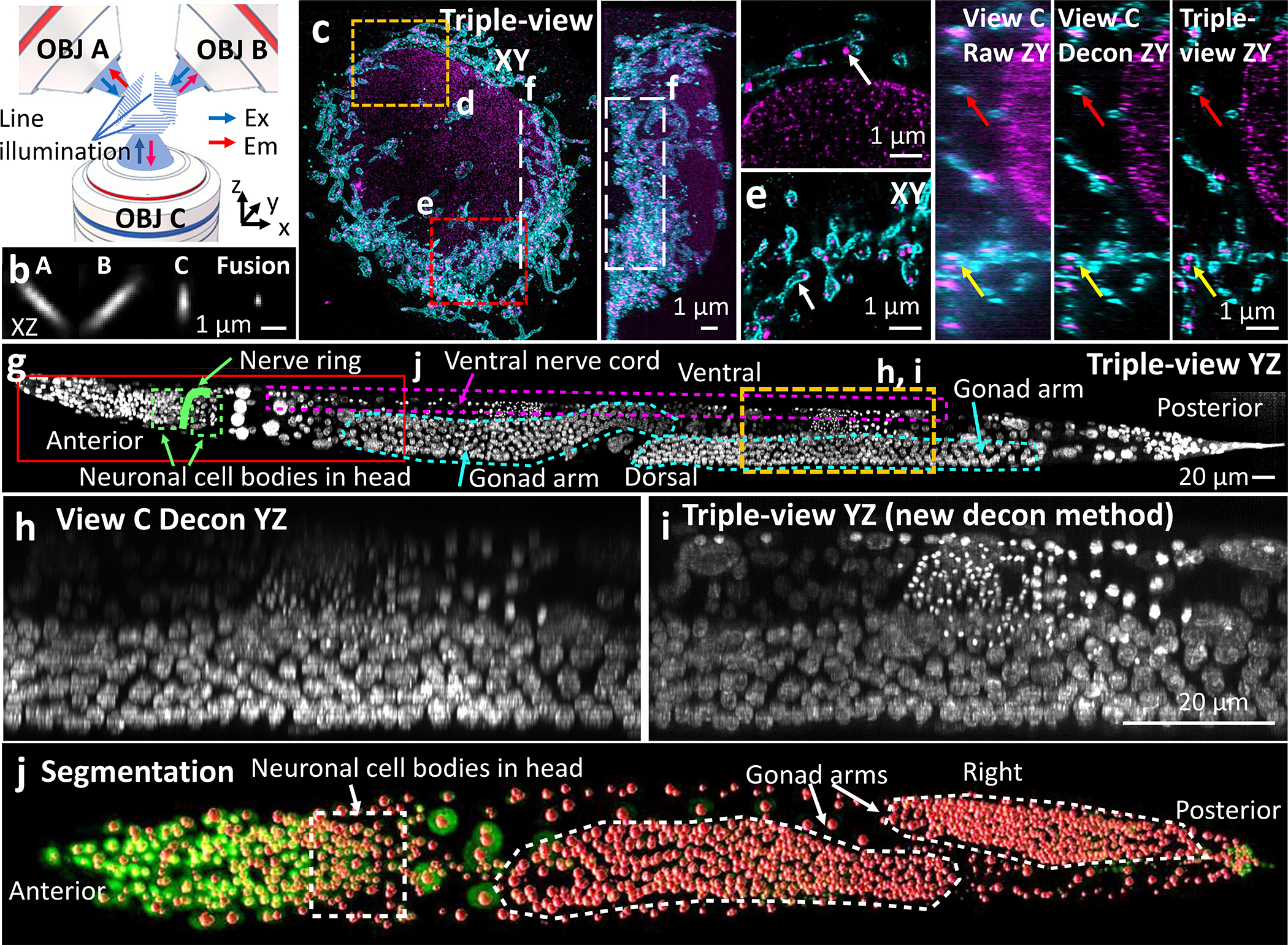
a) Concept. Diffraction-limited line illumination is serially scanned via three objectives (OBJ A/B/C), collecting resulting fluorescence. b) 100 nm beads, raw views and triple-view fusion. c) Triple-view maximum intensity projection (MIP), 4x expanded U2OS cell immunolabeled against mitochondrial outer membrane (cyan, rabbit-anti-Tomm20, goat anti-rabbit Biotin, streptavidin Alexa Fluor 488) and double stranded DNA (magenta, mouse anti-dsDNA and donkey anti-Janelia Fluor 549). d, e) Higher magnification views of regions in c) at 8.6, 2.2 μm depths. Arrows: mitochondrial nucleoids encapsulated within Tomm20 signal. f) Comparative higher magnification views of dashed line/rectangle in c). Red, yellow arrows: mitochondria, nucleoids. See Supplementary Video 1. g) Triple-view axial MIP of whole fixed adult C. elegans, labeled with NucSpot Live 488. h-i) Comparative higher magnification views of yellow rectangular region in g), with bottom deconvolved view h) and attenuation-compensated triple-view deconvolution i). j) Triple-view (green), segmented nuclei overlaid in red, corresponding to rectangular region in g). See Supplementary Video 2. Experiments were repeated on similar datasets twice; representative data from single experiment shown.

We next used our microscope to enhance nanoscale imaging of subcellular structures that were physically expanded to enhance resolution⁹. We expanded fixed U2OS cells immunolabeled to highlight DNA and Tomm20, imaged them from all three views, and reconstructed the triple-view result (Fig. 1c) to clearly resolve sub-organelle detail (Fig. 1d, e). While individual views also offered super-resolution detail due to the expansion procedure (resolution 112±19 nm laterally, 152±38 nm axially), anisotropy distorted the shapes of mitochondria and DNA puncta. Deconvolving individual views offered some improvement (64±8 nm laterally, 100±3 nm axially, n = 10 slices), but less than the triple-view result (54±6 nm laterally, 78±17 nm axially, Fig. 1f, Extended Data Fig. 4a, Supplementary Video 1). In a multicellular example, we fixed and imaged a whole C. elegans L1 larva with a nuclear label, finding the triple-view reconstruction gave clearer views of subnuclear structure over the entire ~250 μm length than individual views (Extended Data Fig. 3c–f).

Despite decades of work on C. elegans, segmenting all nuclei in an intact adult (~30–40 fold larger in volume than an L1) has proven intractable due to increasing scattering and background in the deeper tissues. To investigate if the complementary coverage provided by triple-view imaging would help, we fixed and imaged an adult C. elegans nematode stained for nuclei with NucSpot Live 488, reconstructing the entire worm volume spanning ~871 × 125 × 56 μm³ (Fig. 1g, Extended Data Fig. 5, Supplementary Video 2). As expected, we noticed pronounced depth-dependent attenuation in raw views (Fig. 1h). The same degradation was evident when imaging the sample on a state-of-the-art point-scanning confocal microscope (Extended Data Fig. 5a, e), which was also ~26-fold slower (~70 mins) than our triple-view approach (~160 s). Fusion of the views improved signal at the periphery of the imaging volume, where attenuation is minimal. However, signal in the interior of the animal still appeared dim (Extended Data Fig. 5d). To remedy this, we measured and explicitly incorporated the attenuation in our deconvolution algorithm (Extended Data Fig. 5b). This procedure produced clear reconstructions throughout the sample volume (Fig. 1i), allowing us to employ a deep learning routine^10,11 in conjunction with manual editing, to segment 2136 nuclei in the worm (Fig. 1j, Supplementary Video 2). Such holistic segmentation was impossible using either the point-scanning data or the conventional triple-view fusion.

We also imaged a 30 μm thick tissue section from fixed mouse kidney, immunolabeling four targets to highlight subcellular constituents of glomeruli and convoluted tubules (Extended Data Fig. 6a–d). Again, the triple-view reconstruction provided subcellular detail throughout the volume, while individual views exhibited so much attenuation that cells and blood vessels appeared absent at the far side. Triple-view fusion also produced better reconstructions of nuclear and protein labels in mouse cardiac and brain tissue slices, reminiscent of hematoxylin and eosin stain, but with volumetric information (Extended Data Fig. 6e–j). Finally, we examined the notum region of Drosophila larval wing imaginal discs, confirming that triple-view fusion gave better reconstructions near the top surface of the volume than either single views or higher NA single-view spinning-disk confocal reconstructions of a similar sample (Extended Data Fig. 7).

Deep learning based live confocal imaging

We next applied our multiview system to living samples (Fig. 2). First, we imaged mitochondria and lysosomes in human colon carcinoma (HCT-116) cells (Fig. 2a, Supplementary Video 3). Axial detail in the triple-view reconstructions enabled us to discern transient interactions between organelles that appeared to result in mitochondrial fission (Fig. 2c), otherwise obscured in the raw views (Fig. 2b). Second, we imaged mitochondria in live contractile cardiomyocytes¹² (Supplementary Video 3). Triple-view reconstructions displayed better spatial resolution and contrast than the raw single-view confocal data (Extended Data Fig. 8). However, the cardiomyocyte data also illustrate difficulties with our confocal approach: motion blur, indicating the need for more rapid imaging, and a progressive loss of fluorescence loss over time, indicating photobleaching (Supplementary Video 3).

Fig. 2. Multiview confocal live imaging.

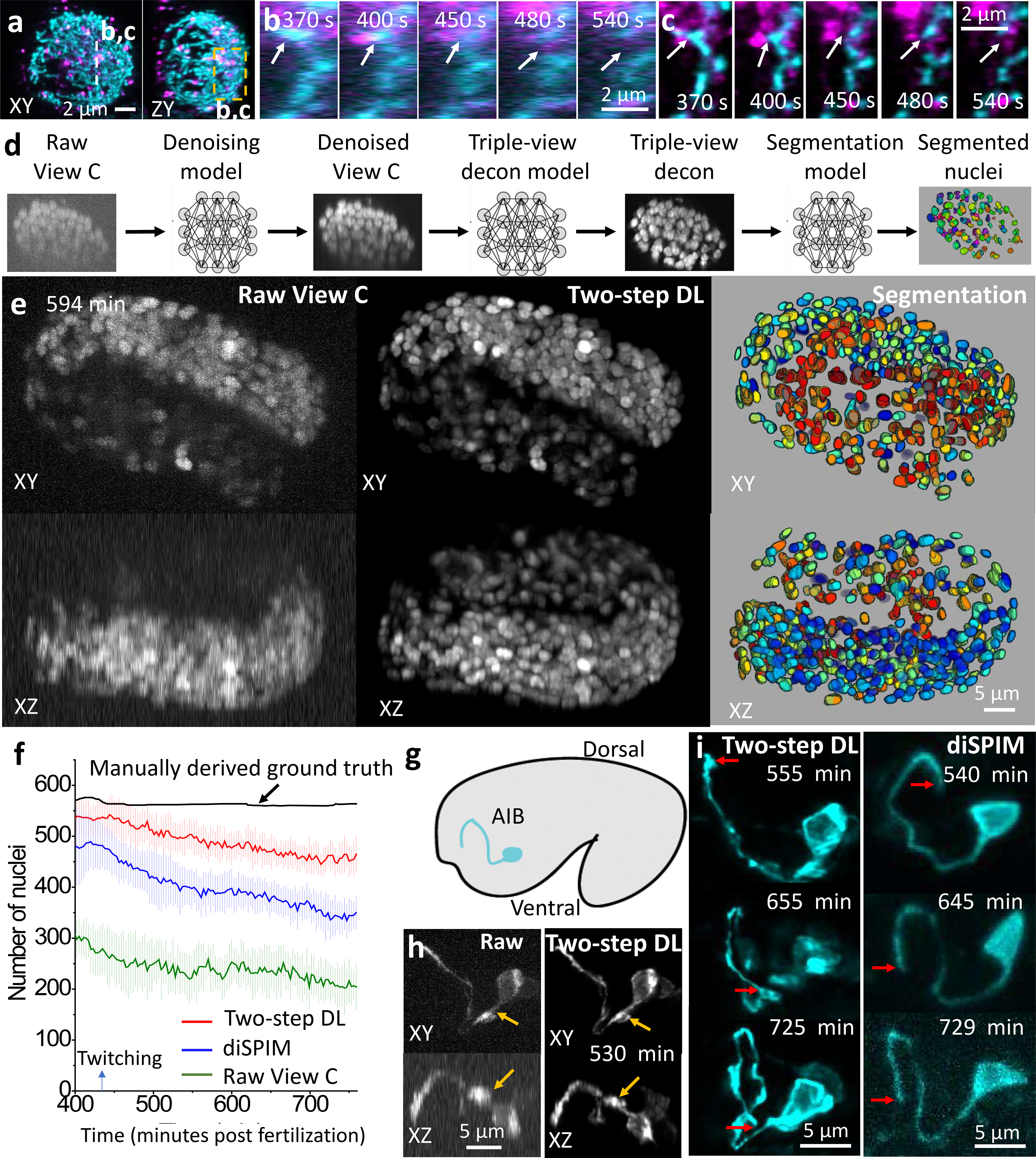
a) HCT-116 human colon carcinoma cells, MitoTracker Green (cyan) and LysoTracker Deep Red (magenta) labels, 1.15 s/three-views, every 10 s, 60 time points. Triple-view lateral, axial MIPs are shown for single time point. b, c) Higher magnification of dashed line/rectangle in a), highlighting association between lysosomes and mitochondria, mitochondrial fission (arrows), comparing single- b) to triple-view c). See Supplementary Video 3. d) Deep learning workflow: three neural networks that denoise, deconvolve, and segment nuclei. e) Example from live C. elegans embryo; H2B-GFP; volumes acquired in 0.6 s, every 3 minutes, 130 volumes. Left: MIPs of View C input. Middle: after two networks. Right: 3D rendering after segmentation. See Supplementary Video 4. f) Nuclear segmentation, twitch to hatch, from View C, diSPIM, View C after two-step DL, and ground truth in ref¹⁵. Means and standard deviations shown from 16 embryos. g) Schematic, AIB neuron in C. elegans embryo. h) Comparative MIPs of AIB marked with membrane targeted GFP, volumetrically acquired in 0.75 s, every 5 min, 65 volumes. Arrows: features better resolved after DL. Neurite widths (mean ± standard deviation) in raw data: 470±17 nm laterally, 1268±127 nm axially; after DL: 355±17 nm laterally and 754±46 nm axially (n = 10 time points). i) Comparisons of two-step DL vs. diSPIM highlighting developmental elaboration of AIB neurite tip (arrows). Experiments repeated 3 times for a), 16 times e-f), 10 times g-i); representative data from single experiments shown.

The necessity for rapid imaging and minimal phototoxicity is more stringent when imaging developing animals, e.g. C. elegans embryos¹³. Motion blur, photobleaching, developmental delay or embryonic arrest confounded our attempts to obtain high signal-to-noise ratio (SNR) triple-view recordings of a pan-nuclear, GFP-histone label over the seven-hour period from embryonic twitching to hatching. To address this, we implemented sequential neural networks¹⁴ that (1) denoised the raw, low SNR lower view recordings and then (2) predicted the high SNR triple-view output, given the higher SNR single-view confocal prediction (Fig. 2d, Extended Data Fig. 9a). Intriguingly, this two-step approach produced better output than using a single network to predict high SNR triple-view output directly from noisy single-view raw data (Extended Data Fig. 9b, d).

An advantage of the C. elegans system is that the number of nuclei can be exactly scored by manually inspecting many embryos¹⁵. This has not been repeated in a single embryo due to imaging challenges. Indeed, inspection of the noisy single-view input revealed that scattering severely attenuated the signal of nuclei on the ‘far side’ of the embryo. Qualitatively, the two-step prediction appeared strikingly better than the single-view input, restoring many nuclei even at increasing depths (Fig. 2e, Supplementary Video 4). To quantify the improvement, we then used a third neural network (Fig. 2f, Extended Data Fig. 9e, f), to segment and count the number of nuclei. Against the ground truth, the raw single confocal view found fewer than half of all nuclei. The two-step prediction fared much better, capturing the majority of the nuclei, outperforming single-view light-sheet microscopy data passed through a neural network designed to improve resolution isotropy⁵, and even dual-view light-sheet microscopy data (diSPIM^16–18, Fig. 2f, Extended Data Fig. 9g).

Next, we applied our two-step restoration method to study neurite development in the C. elegans nerve ring, the equivalent of the nematode brain (Fig. 2g). We focused our analyses on the AIB interneurons, a pair of “functional hub”¹⁹ neurons which bridge communication between modular, distinct regions of the neuropil.²⁰ While the morphology of AIB is well known, the developmental events leading to its precise positioning in the brain remain unknown. The two-step prediction improved SNR, resolution, and contrast relative to raw single-view input data (Fig. 2h, Extended Data Fig. 9c). We also compared two-step predictions to another embryo imaged over the same period with diSPIM (Fig. 2i, Extended Data Fig. 4b). The superior resolution of the prediction enabled us to detect growth cone dynamics at the tip of the neurite and the emergence of presynaptic boutons as the neurite engaged with its postsynaptic partners. Fluorescent intensity in the labeled growth cone²¹ decreased as the AIB neurite was correctly positioned into its final neighborhood, concomitant with the emergence (and increasing intensity) of presynaptic boutons, indicating a developmental transition during synaptogenesis. Other imaging approaches, including diSPIM, were incapable of capturing these subcellular structural changes (Extended Data Fig. 9h).

Multiview super-resolution imaging

The size discrepancy between the diffraction-limited point spread function (PSF) and a fluorescently labeled target hinders subcellular observation. To ameliorate this problem, we integrated super-resolution methods into our imaging platform. We reasoned that the diffraction-limited line structure in our microscope could be used for structured illumination microscopy (SIM²²), provided we modified our acquisition scheme to isolate sparse fluorescence emission in the vicinity of the line focus (Extended Data Fig. 10). Scanning the line illumination along three orthogonal directions (Fig. 3a) and collecting and processing five images per direction then enabled three-dimensional super-resolution imaging, improving volumetric resolution 5.3-fold, from 335 × 285 × 575 nm³ to 225 × 165 × 280 nm³ in triple-view 1D SIM mode (Extended Data Fig. 10).

Fig. 3. Multiview super-resolution microscopy.

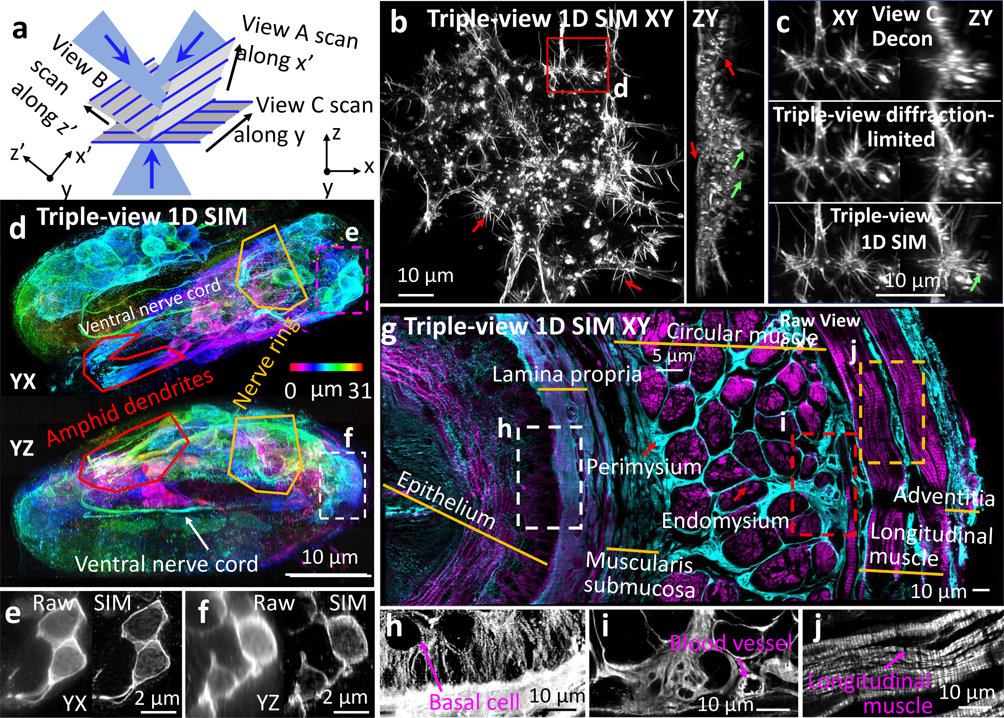
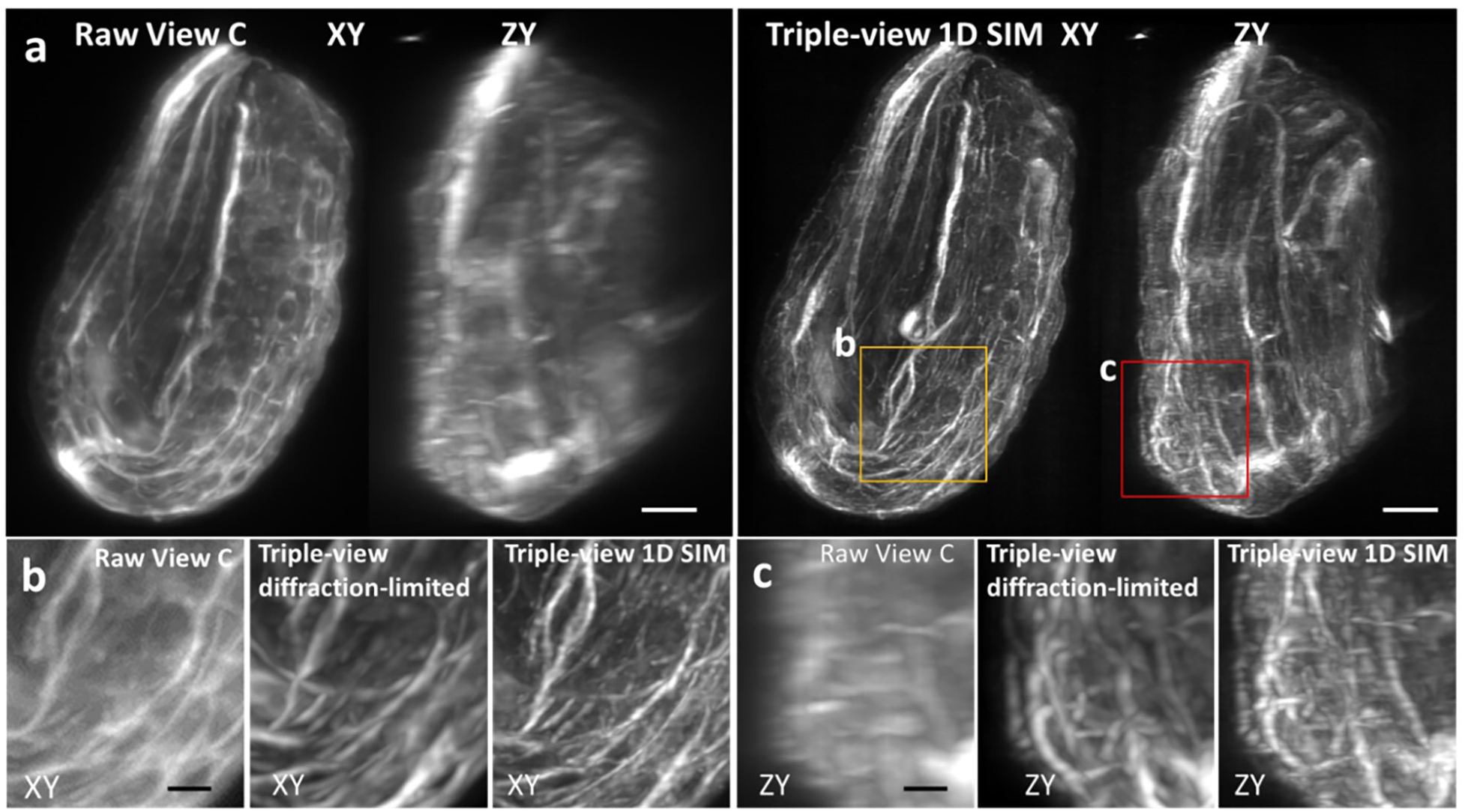
a) Illumination geometry. Sparse, periodic line illumination is scanned in orthogonal directions (x’, y, z’), enhancing 3D resolution. b) Triple-view 1D SIM MIPs, fixed B16F10 mouse melanoma cells, Alexa Fluor 488 phalloidin label, embedded in 1.8% collagen gel. Red/green arrows highlight filopodia/invadopodia. c) Comparative higher magnification views of rectangular region in b). See Supplementary Video 5. d) Triple-view 1D SIM MIPs from fixed, 3.3-fold expanded C. elegans embryo, immunostained with rabbit-anti-GFP, anti-rabbit-biotin, streptavidin Alexa Fluor 488 to amplify GFP marking neuronal structures. Images depth coded as indicated. Comparative higher magnification lateral (e), axial (f) views indicated by rectangles in d). g) Triple-view 1D SIM XY image, mouse esophageal tissue slab (172 × 365 × 25 μm³), tubulin (mouse-anti-alpha tubulin, anti-mouse JF 549, cyan) and actin (phalloidin Alexa Fluor 488, magenta) stains. h-j) Higher magnification single-color views of white (h, tubulin), red (i, tubulin), and orange (j, actin) regions in g), anatomical features highlighted. Contrast adjusted in h) to visualize outline of basal cell. Experiments repeated 5 times for b), 2 times for d) and g); representative data from single experiment shown.

An advantage of this SIM implementation is its ability to interrogate thick, densely labeled samples due to strong suppression of out-of-focus light. For example, when imaging Alexa Fluor 488 phalloidin-labeled actin in fixed B16F10 mouse melanoma cells embedded in a 1.8% collagen gel²³, the triple-view 1D SIM reconstruction offered clearer views of three-dimensional actin-rich filopodia and invadopodia (Fig. 3b) than diffraction-limited single- or triple-view results (Fig. 3c, Extended Data Fig. 4c, Supplementary Video 5). We observed similar gains on fixed and immunolabeled C. elegans embryos (Extended Data Fig. 11). We also compared the triple-view 1D SIM to instant SIM²⁴, a rapid single-view SIM implementation, on a fixed, collagen gel embedded HEY-T30 ovarian cancer cell dual-labeled for actin and mitochondria (Extended Data Fig. 12a, b). Although lateral resolution was similar, our triple-view method provided better axial resolution.

Triple-view 1D SIM also improved reconstructions of 4x expanded U2OS cells immunostained for Tomm20 and microtubules relative to single-view input (Extended Data Fig. 12c, d). To investigate performance in expanded multicellular samples, we adapted and optimized methods^25,26 to expand C. elegans embryos 3.3-fold (Extended Data Fig. 13), using triple-view 1D SIM to visualize amphid neurites, the nerve ring, and ventral nerve cord (Fig. 3d). Comparisons on cellular membranes with raw single- and triple-view data highlighted the improvement offered in the SIM mode (Fig. 3e, f, Extended Data Fig. 4d).

Finally, we applied triple-view 1D SIM imaging to a slab of fixed mouse esophageal tissue with immunolabeled actin and microtubules. At larger scales (Fig. 3g), we identified distinct, radially arranged anatomic regions, including epithelia, lamina propia, submucosa, perimysium, endomysium, longitudinal muscle and adventitial tissue layers. At smaller scales, the subcellular detail afforded by our reconstruction also enabled crisp visualization of cells, small vessels, and the striated, periodic actin arrangements within longitudinal muscle (Fig. 3h–j).

Deep learning for dynamic 3D SIM imaging

Triple-view 1D SIM requires 15x as many images as conventional single-view CM, hampering live super-resolution applications. To address this, we began by training a residual channel attention network (RCAN²⁷) to predict 1D super-resolved images from diffraction-limited input. If training data is assembled from samples arranged in random orientations (typical when imaging biological specimens), we reasoned that 1D resolution could also be improved in any direction simply by rotating the input image and reapplying the trained neural network. Combining all such rotated, super-resolved views^16,28 then enables isotropic, 2D resolution enhancement (Fig. 4a) from a single confocal image. We validated this approach using phantom objects (Extended Data Fig. 14)²⁷, then applied it to images of immunolabeled microtubules (Fig. 4b, Extended Data Fig. 15), finding filaments were better resolved (176±8 nm, n = 10 xy slices) than with either the initial 1D SIM network output or the confocal input (386±42 nm).

Fig. 4. Deep learning enhances multiview super-resolution imaging.

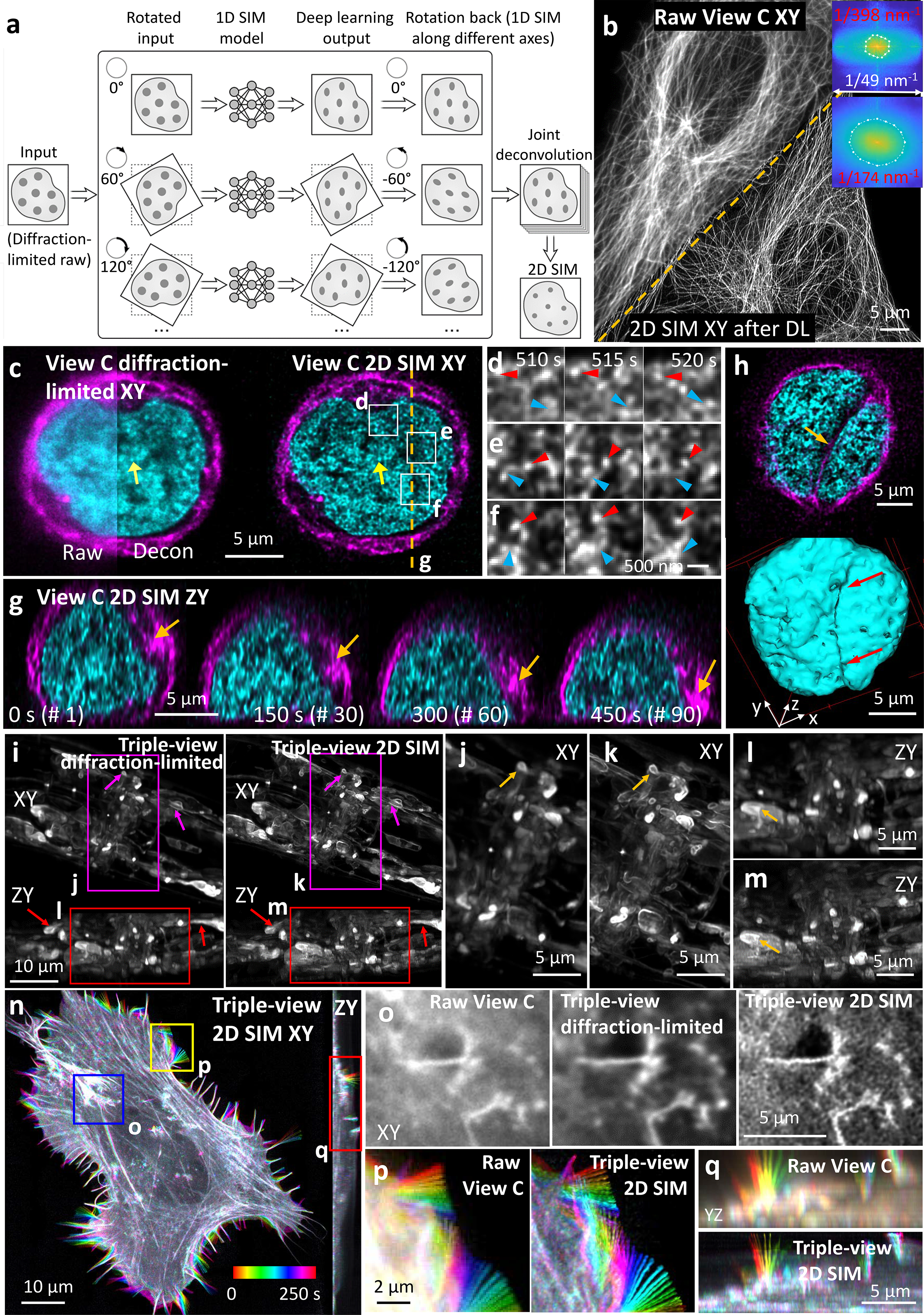
a) Deep learning, joint deconvolution produce 2D super-resolution images from diffraction-limited input. b) CM volumes of immunolabeled microtubules before and after 2D SIM predictions. Inset: Fourier transforms show resolution improvement to ~170 nm after prediction. c) Comparative lateral plane within Jurkat T cell expressing H2B-GFP (cyan), EMTB-mCherry (magenta), volumes every 5 s, 200 time points. Arrows: fine nuclear structure. Decon: deconvolved. d-f) Higher magnification views of rectangular regions in c), red arrowheads: the same H2B nanodomain; blue arrowheads: splitting, merging of H2B nanodomains. g) Axial plane corresponding to dashed line in c), highlighting centrosome movement towards coverslip (arrow) and accompanying nuclear shape distortion. See Supplementary Video 6. h) Lateral plane (top) and surface rendering (bottom) of nuclear indentation by microtubule bundles. i) MIPs from anesthetized L4 larval worm expressing membrane targeted GFP, comparing dense nerve ring region, triple-view diffraction-limited vs. triple-view 2D SIM. Higher magnification lateral (j, k) and axial (l, m) views of regions in i), arrows indicate regions for comparison. See Supplementary Video 7. n) Example 2D SIM MIP of U2OS cell expressing Lifeact tdTomato, volumes every 10 s, 100 time points. Images color coded to indicate temporal evolution. o-q) Comparative higher magnification view of blue, yellow, red regions in n), color coded to illustrate filopodial dynamics. See Supplementary Video 8. Experiments repeated 4 times for b), 2 times c-h) and n-r), and 3 times i-m); representative data from single experiment shown.

We next imaged live Jurkat cells transiently transfected with microtubule and actin markers, and activated on antibody-coated coverslips, recording 150 volumes at two second intervals. Applying our method improved resolution and contrast relative to the confocal input, resolving ruffling actin dynamics at the periphery and microtubule dynamics closer to the T cell center (Extended Data Fig. 16a, Supplementary Video 6). We also applied the method to T cells expressing histone and microtubule markers, recording 200 volumes at 5 second intervals during activation (Supplementary Video 6). The superior resolution offered by the 2D SIM output revealed H2B nanodomains that were obscured in the confocal input and barely evident after deconvolution (Fig. 4c, Extended Data Fig. 4e). Close inspection revealed dynamic nanodomain splitting and merging (Fig. 4d–f), consistent with 2D observations of ‘chromatin blobs’ imaged in live U2OS cells²⁹. We visualized relocation of the centrosome towards the cell-substrate contact zone in axial views; concomitant squeezing and deformation of the nucleus as the cell spread on the activating surface (Fig. 4g, Extended Data Fig. 16b); indentation of the nucleus near microtubule bundles (Fig. 4h); the tight wrapping of microtubules around the nucleus (Extended Data Fig. 16c); and a concave nuclear deformation produced by the centrosome, pulling and rotating the nucleus as it docked at the immune synapse (Extended Data Fig. 16b).

Applying deep learning to enhance resolution in each view enables a highly versatile imaging platform, facilitating comparisons between different microscopy modes (Extended Data Fig. 17, Supplementary Table 1, Fig. 4i–q). First, we imaged a fixed, 18 μm thick L2 stage C. elegans larva expressing a GFP membrane marker primarily in the nervous system (Extended Data Fig. 18a). Compared to the lower confocal view, the triple-view 1D SIM reconstruction derived from 15 input volumes improved resolution and contrast, and applying the RCAN to each raw confocal view enabled us to derive a triple-view 2D SIM reconstruction, closely resembling the triple-view 1D SIM reconstruction despite requiring only 3 input volumes (Extended Data Fig. 18b, c). Both triple-view 1D- and 2D SIM reconstructions outperformed a commercial SIM system, which displayed artifacts arising from out-of-focus background (Extended Data Fig. 18e). Second, we imaged the densely labeled nerve ring region in an anesthetized, 28 μm thick L4 stage C. elegans larva embedded in a polymer gel³⁰. The 2D SIM prediction was obviously sharper than the confocal input, better resolving cell bodies and fine neural structure, including membrane protrusions (Extended Data Fig. 18d). Compared to iSIM, the 2D SIM prediction provided similar lateral but better axial views of the specimen (Extended Data Fig. 18d), perhaps due to superior suppression of out-of-focus background. However, all single-view methods suffered worsened image quality at the far side of the larvae. To remedy this, we also acquired the other two confocal views, using them to obtain triple-view deconvolved and 2D SIM reconstructions (Fig. 4i, j). As expected, the triple-view 2D SIM mode offered superior resolution in lateral and axial views (Fig. 4k–m, Supplementary Video 7), a more than ten-fold volumetric improvement compared to the raw confocal data (Extended Data Fig. 17c). Finally, we reconstructed actin dynamics in a U2OS cell, imaging three views every 10 s for 100 time points (Fig. 4n, Supplementary Video 8). Lateral views confirmed the progressive increase in resolution (Extended Data Fig. 17d) from the raw lower view to triple-view 2D SIM output (Fig. 4o, p), with axial views of the latter showing much clearer views of fine filopodial dynamics (Fig. 4q) and retrograde flow (Supplementary Video 8).

Discussion

Here we synergize concepts from multiview imaging and SIM to improve performance relative to state-of-the-art CM and SIM²². Our work provides a blueprint for the integration of deep learning with fluorescence microscopy, as we used neural networks to extend imaging duration and depth, and produce super-resolution images from diffraction-limited input images. Importantly, the latter capability does not degrade temporal resolution or introduce more dose relative to the input images. The same approach could likely be applied to other microscopes with line illumination^31–34, possibly enabling better spatial resolution than achieved here.

We envision several extensions to our work. First, the three objectives here were chosen to image a wide range of sample sizes. For studying single cells, higher spatial resolution can be easily attained by using higher NA lenses³⁵. Second, our success imaging expanded samples suggests that other cleared tissue⁵ would also benefit from our methods. Third, employing longer wavelength, multiphoton illumination would further improve imaging in thick samples. Fourth, five-fold faster SIM imaging is possible using optical reassignment³⁶; and faster and more light-efficient multiview imaging may be realized by simultaneously recording from all three views, using deconvolution^5,35 to compensate for the resulting spatially varying PSF. Fifth, if the line-scanners were modified for lower illumination NA, converting them into light-sheets, cross-modality deep learning techniques^27,37 could be used to improve spatial resolution in light-sheet microscopy. Finally, we did not correct sample-induced aberrations. Incorporating adaptive techniques³⁸ that dynamically measure and correct these aberrations could improve imaging in large, heterogenous samples, as demonstrated in light-sheet^39,40 and super-resolution microscopy⁴¹.

Extended Data

Extended Data Fig. 1, Instrument overview.

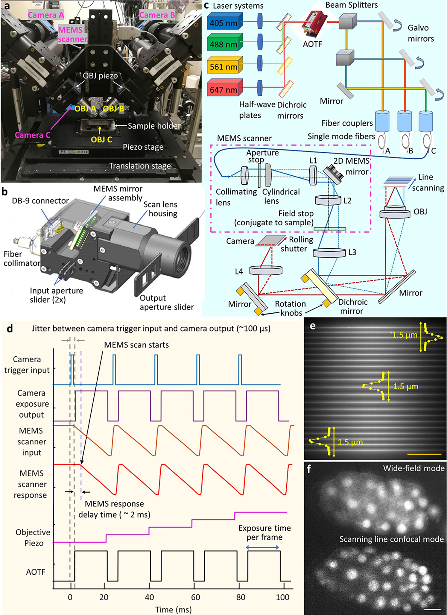
a) Photograph of instrument, highlighting objectives, cameras, sample area. b) CAD rendering of MEMS line scanner. c) Optical setup. Diode lasers are combined and passed through an acousto-optic tunable filter (AOTF) for shuttering and power control, before being directed into broadband single-mode fibers. Galvanometric mirrors are used to direct beams into each fiber, and to adjust the power of the beams entering the fiber. Each fiber is then fed into a MEMS line scanner (purple dot-dashed line, here only one shown for clarity), with optics as indicated. The scanner serves to collimate the fiber output, focus it with a cylindrical lens, scan it with a MEMS mirror, and image the scanned output to a field stop at a conjugate sample plane. The beam is then relayed via lens L3 and the objective to the sample plane, after reflection from a dichroic mirror. Fluorescence is collected in epi-mode, transmitted through a dichroic mirror, and imaged via tube lens L4 onto a scientific CMOS camera where it is synchronized to the rolling shutter readout. d) Control waveforms issued to camera, MEMS scanner, objective piezo, and AOTF, used to acquire volumetric data. See also Supplementary Methods. e) Example line illumination at various lateral positions on camera chip, as imaged with fluorescent dye in lower view C. Excitation PSF measurements are taken at various positions in the field (see also Extended Data Fig. 2a, c). Scale bar: 50 μm. f) Example images acquired in C. elegans embryo expressing GFP-histones, as visualized in bottom view C with widefield mode (top) and line-scanning mode (slit width 0.58 μm, bottom). Scale bar: 5 μm.

Extended Data Fig. 2, Further characterization of imaging field.

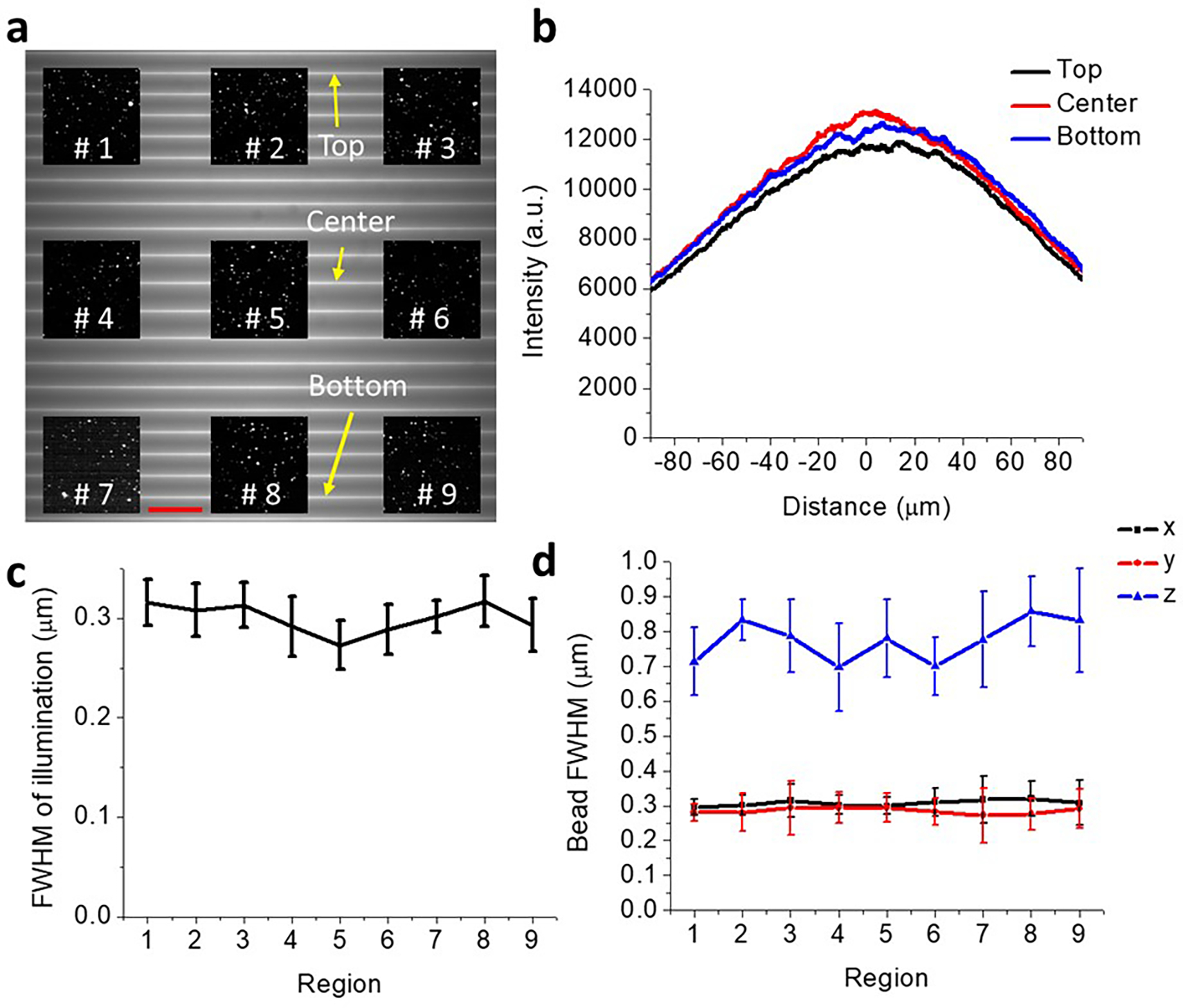
a) 175 × 175 μm² imaging field, showing representative horizontal illumination lines across field, as measured in fluorescent dye. Also superimposed are example regions of interest (#1 - #9) from a separate experiment, showing images of 100 nm fluorescent beads at different field locations. Scale bar: 20 μm. b) Excitation uniformity measured along the long axis of illumination, from lines at top, middle, and bottom of imaging field, as marked in a). c) Full width at half maximum (FWHM) of short axis of illumination line, as measured at regions in a). FWHMs are estimated by scanning illumination relative to bead and recording intensity as a function of scan position. Means and standard deviations derived from 15 beads are reported at each location. d) As in c), but now reporting x, y, and z FWHMs derived from images of individual beads (n = 15).

Extended Data Fig. 3,

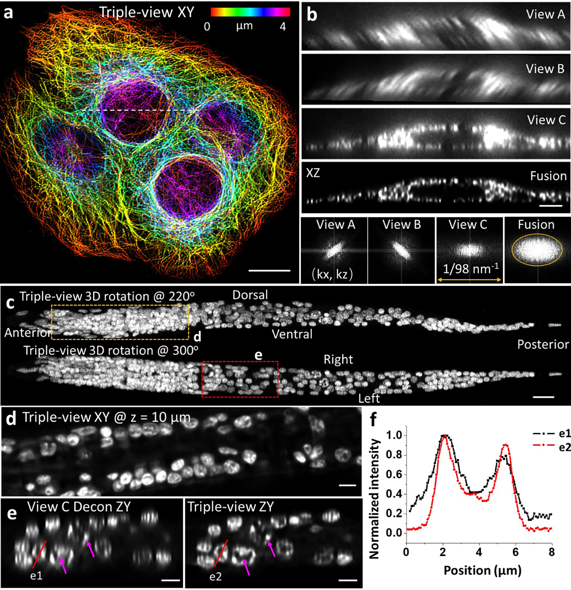
a) Lateral maximum intensity projection image of fixed U2OS cells immunolabeled with mouse-anti-alpha tubulin, anti-mouse-biotin, streptavidin Alexa Fluor 488, marking microtubules (fused result after registration and deconvolution of all three raw views). Height: color bar. b) Raw and fused axial views along the dashed line in a). Fourier transforms of axial view are shown in last row, showing resolution enhancement after fusion. Orange oval: 1/260 nm⁻¹ in half width and 1/405 nm⁻¹ in half height. c) Triple-view reconstruction of whole fixed L1 stage larval worm, nuclei labeled with NucSpot 488. Two maximum intensity projections are shown, taken after rotating volume 220 degrees (top) and 300 degrees (bottom) about x axis. d) Higher magnification lateral view 10 μm from the beginning of the volume, corresponding to the yellow dashed region in c). e) Higher magnification axial views (single planes) corresponding to the red rectangular region in c), comparing single-view deconvolved result (left) to triple-view result (right). Magenta arrows highlight subnuclear structure better resolved in triple-view result. f) Line profiles corresponding to e1, e2 in e). Scale bars: a, c) 10 μm; b, e) 3 μm.

Extended Data Fig. 4, Contrast and resolution is enhanced after multiview fusion or SIM.

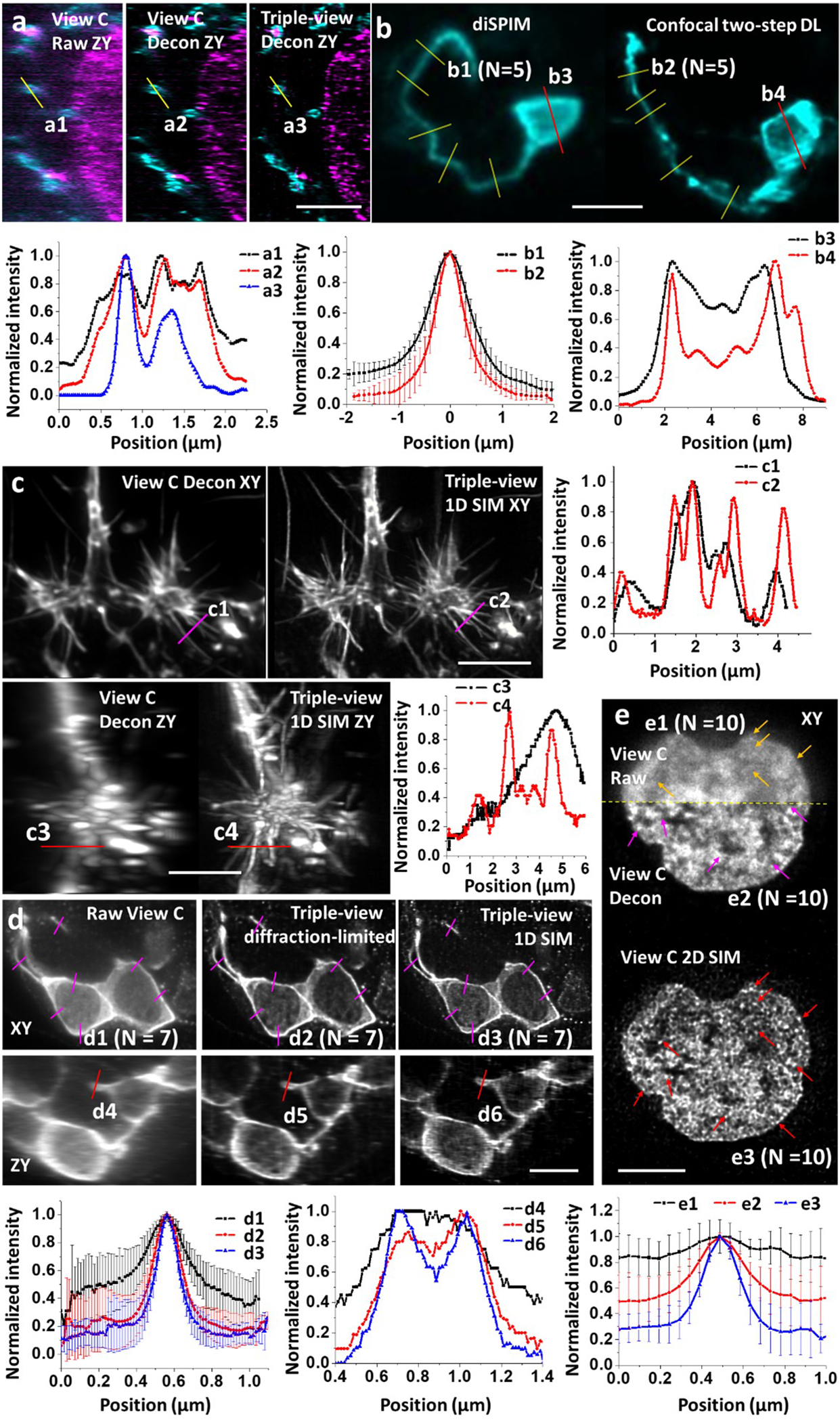
a) Nanoscale imaging of organelles (mitochondrial outer membrane, cyan; and double stranded DNA, magenta) in expanded U2OS cells, to accompany Fig. 1f. Top: images, bottom: line profiles corresponding to a1-a3 at top. b) Neurons marked with membrane targeted GFP in living C. elegans embryos, to accompany Fig. 2i. Top: images; bottom: line profiles corresponding to b1-b4 at top, n = 5 profiles at indicated positions were used to generate means +/− standard deviations for b1, b2. c) Stained actin in fixed B16F10 mouse melanoma cells embedded in collagen gels, to accompany Fig. 3c. Left: images; right: line profiles corresponding to c1-c4 at left. d) Neurons in fixed, expanded C. elegans embryos, to accompany Fig. 3e, f. Top: images; bottom: line profiles corresponding to d1-d6 at left, n = 7 profiles at indicated positions were used to generate means +/− standard deviations for d1-d3. e) H2B puncta in live Jurkat T cells, to accompany Fig. 4c. Top: images; bottom: line profiles corresponding to e1-e3 at top, n = 10 profiles at indicated positions were used to generate means +/− standard deviations for e1-e3. Scale bars: a, d) 2 μm, b, c, e) 5 μm.

Extended Data Fig. 5, Triple-view comparisons in adult C. elegans.

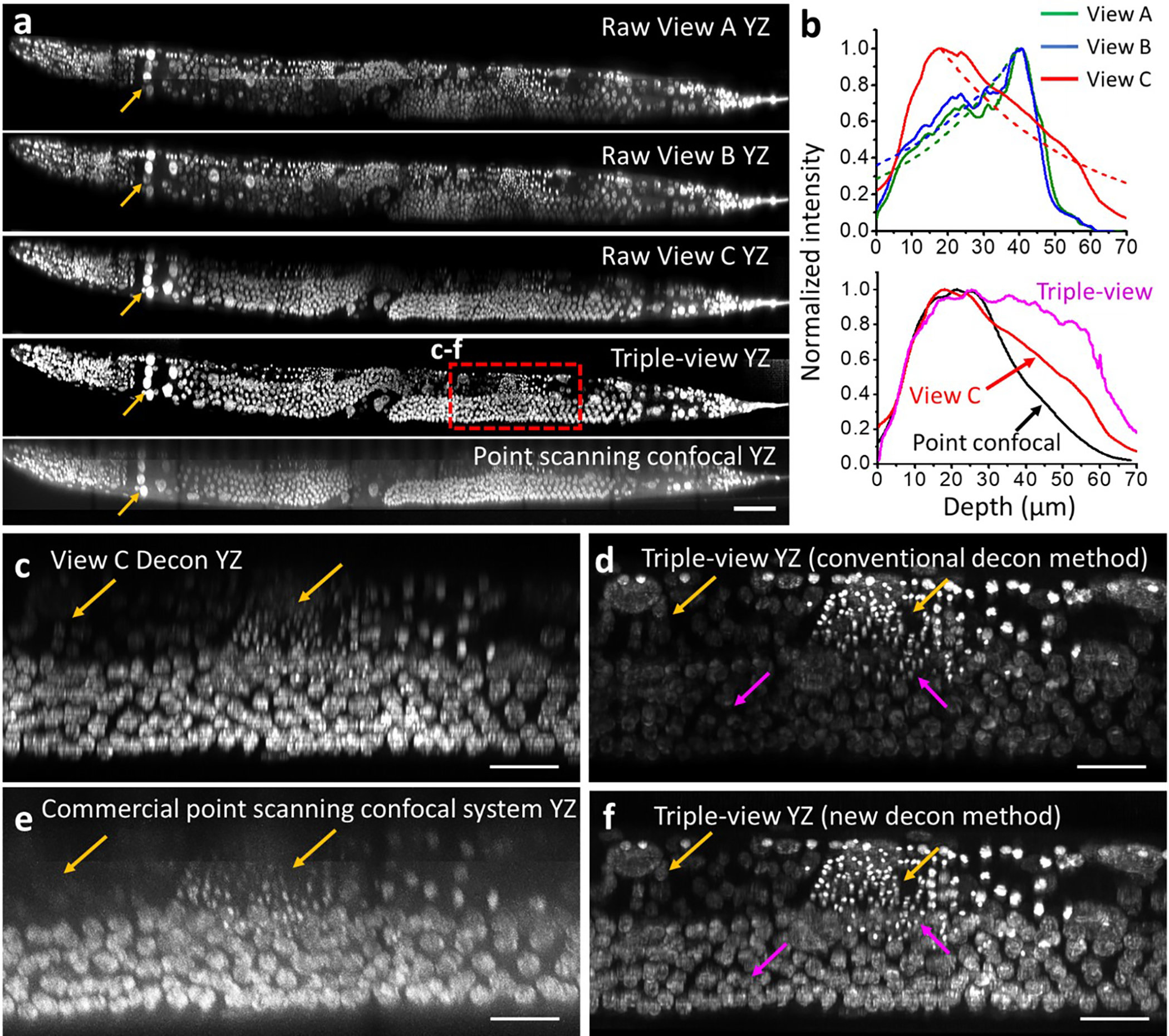
a) Axial views of whole fixed worm labeled with NucSpot Live 488, comparing raw views gathered by objectives A, B, C; triple-view reconstruction; and point-scanning confocal microscope. Arrows highlight example region with uniformly good quality in triple-view reconstruction, but showing attenuation either at bottom (Views A, B) or top (View C, point-scanning confocal) of stack with other methods. See also Fig. 2g–j. b) Average attenuation measured through axial extent of the worm, as measured by raw views A, B C (top graph) and triple-view reconstruction and point-scanning confocal (bottom graph). Exponential fits to the data are also shown with dashed lines. See also Supplementary Methods. c-f) Comparative higher magnification views of dashed red rectangular region in a), with bottom deconvolved view c), commercial Leica SP8 confocal microscope e), conventional triple-view deconvolution d), attenuation-compensated triple-view deconvolution f). Colored arrows highlight comparisons, orange: single- vs. triple-view, magenta: deconvolution methods. Scale bar: a) 50 μm, c-f) 10 μm.

Extended Data Fig. 6, Triple-view comparisons in scattering tissue.

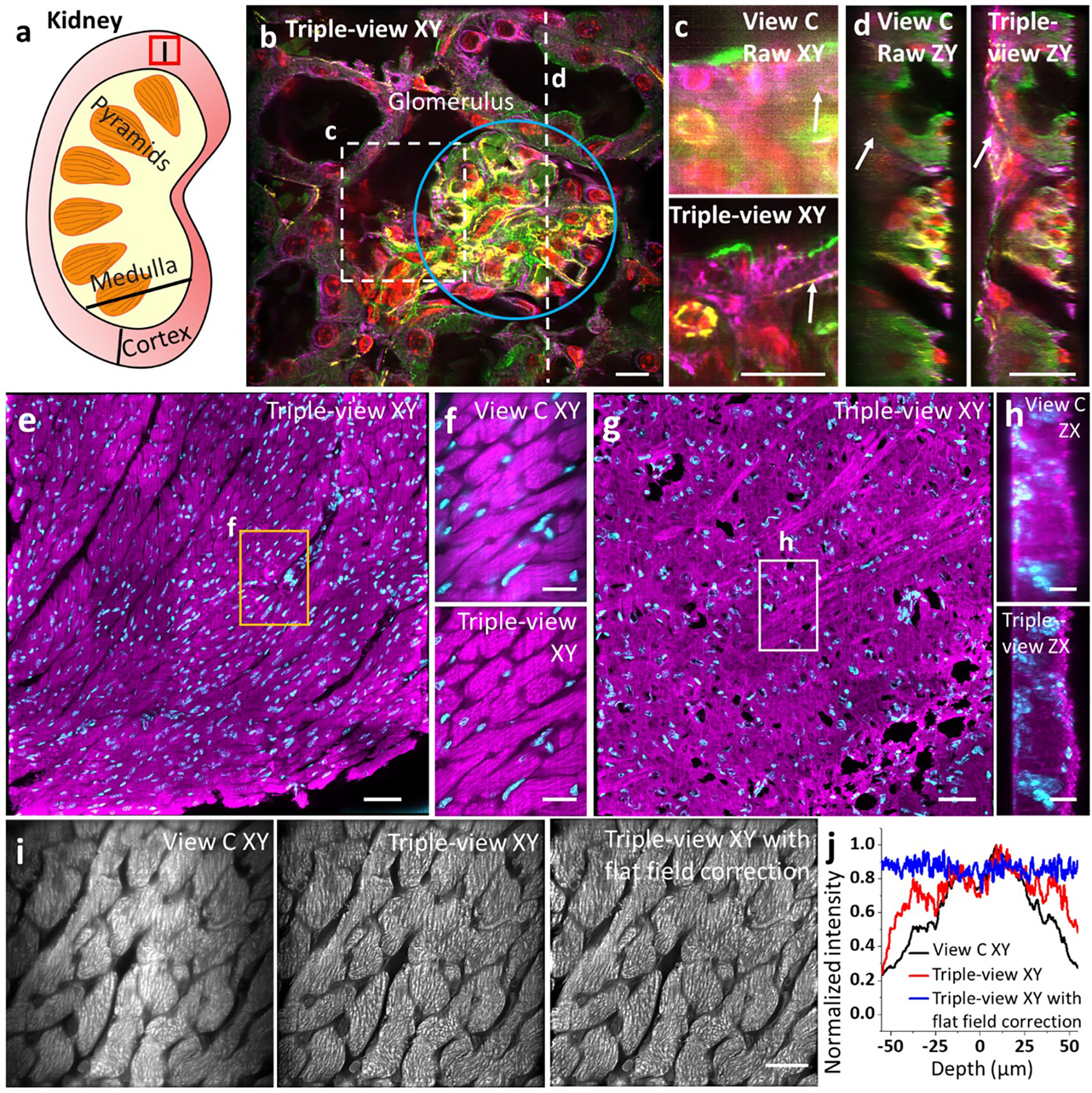
a) Schematic of kidney: approximate region where tissue was extracted. b) Four color triple-view reconstruction of mouse kidney slice. Lateral image at 4 μm depth, highlighting glomerulus surrounded by convoluted tubules. Red: nuclei stained with DAPI, green: actin stained with phalloidin-Alexa Fluor 488; magenta: tubulin immunolabeled with mouse-α-Tubulin primary, α-Mouse-JF549 secondary; yellow: CD31 immunolabeled with Goat-α-CD31 primary, α-Goat AF647 secondary. Scale bar: 20 μm. c) Comparative higher magnification of white rectangular region in b) at 28 μm depth. Scale bar: 20 μm. d) Comparative axial view along dashed line in b). White arrows: structures that are dim in single-view but restored in triple-view. Scale bar: 20 μm. e) Triple-view reconstruction of mouse cardiac tissue (~536 × 536 × 37 μm³ section, shown is a maximum intensity projection of axial slices from 10–30 μm). Magenta: Atto 647 NHS, nonspecifically marking proteins, cyan: NucSpot Live 488, marking nuclei. Scale bar: 50 μm. f) Higher magnification view of orange rectangular region in e), comparing raw View C (top) to triple-view reconstruction (bottom). Scale bar: 20 μm. g) Labels as in e) but showing triple-view reconstruction of mouse brain tissue (~536 × 536 × 25 μm³ section, shown is a maximum intensity projection of axial slices from 5–15 μm). Scale bar: 50 μm. h) Axial maximum intensity projection computed over 120 μm vertical extent of white rectangular region shown in g), comparing raw View C (top) to triple-view (bottom) result. Scale bar: 10 μm. i) Mouse cardiac tissue stained with Atto 647 NHS (same sample as e), nonspecifically marking proteins, as observed in lower view C (left), after triple-view deconvolution (middle), and triple-view deconvolution after flat-fielding (right). Scale bar: 20 μm. j) Intensity profiles from i), created by averaging across vertical axis.

Extended Data Fig. 7, Triple-view comparisons in Drosophila wing imaginal disks.

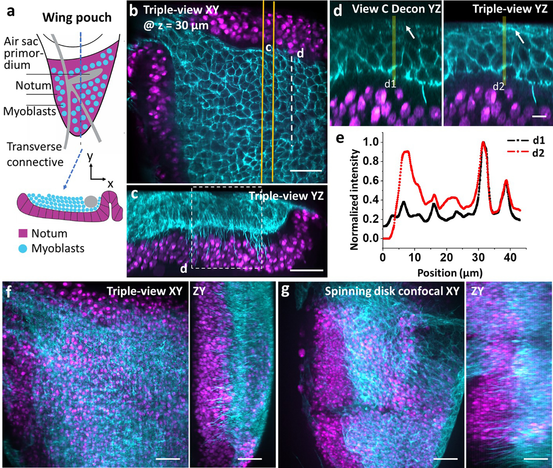
a) Schematic of larval wing disc, lateral (top) and axial (bottom) views, including adult muscle precursor myoblasts and notum. b) Lateral plane from triple-view reconstruction, 30 μm from sample surface. Notum nuclei (NLS-mCherry, magenta) and myoblast membranes (CD2-GFP, cyan) labeled. c) Axial maximum intensity projection derived from 6 μm thick yellow rectangle in b). d) Higher magnification view of white dashed line/rectangle in b/c), comparing single View C deconvolution (left) to triple-view result (right). White arrows: membrane observed in triple-view but absent in single-view. e) Line profiles corresponding to d1, d2 in d). f) Lateral (left) and axial (right) maximum intensity projections of the larval wing disc. g) As in f) but showing another larval wing disc imaged with a spinning-disk confocal microscope with NA =1.3. Scale bars: b, c) 20 μm, d) 5 μm, f, g) 15 μm.

Extended Data Fig. 8, Live triple-view confocal imaging of Cardiomyocytes.

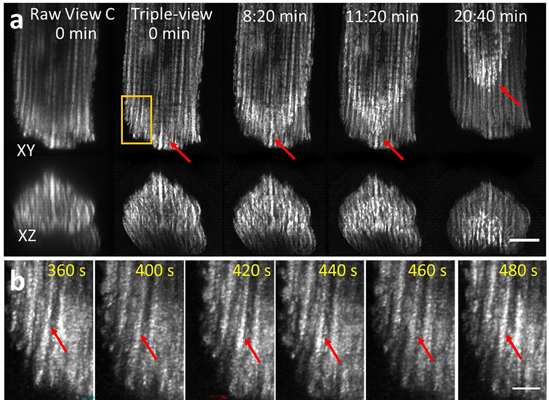
a) Cardiomyocytes expressing EGFP-Tomm20, labeled with MitoTracker Red CMXRos, imaged with triple-view CM in 2.03 s, every 20 s, for 100 time points. Lateral (top) and axial (bottom) maximum intensity projections shown at indicated times before and after registration/deconvolution. Scale bar: 10 μm. b Higher magnification view of orange rectangular region in a), highlighting mitochondrial fluctuations (red arrows) over time. Scale bar: 3 μm. See also Supplementary Video 3.

Extended Data Fig. 9, Neural network schematics.

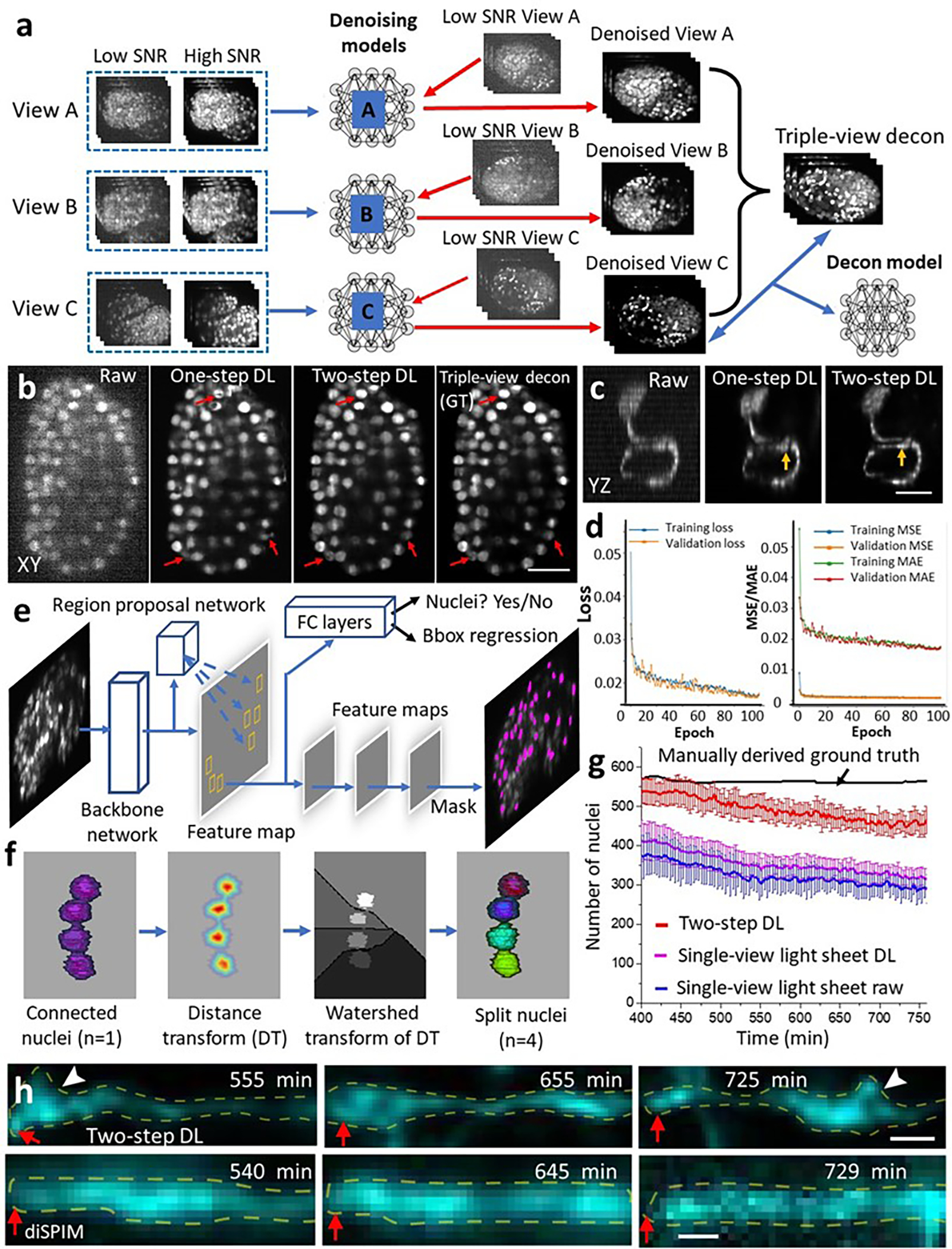
a) Workflow for two-step deep learning procedure used in Fig. 2e–i. Denoising neural networks are trained for views A, B, C, by using matched high and low SNR volumes derived from embryos paralyzed with sodium azide. The denoising output of each model are combined with joint deconvolution (triple-view decon) and are combined with the denoised view C output to train a second neural work (Decon model). In this manner, noisy raw data from View C can be transformed into a high SNR, high resolution prediction. b) Example data (lateral slice through GFP-histone expressing C. elegans embryo) from left to right: raw View C data; single neural-network prediction (raw input View C to high SNR, triple-view deconvolved result); two-step denoised and deconvolved prediction; high SNR denoised triple-view deconvolved result (i.e., ground truth used in training the second neural network in a)). The two-step prediction is noticeably closer to the ground truth (red arrows highlight regions for comparison; 3D SSIM 0.89±0.05, PSNR 43.4±2.2 (mean ± standard deviation, n = 7 embryos) than the single network (3D SSIM 0.72±0.17, PSNR 27.8±6.4, n = 7). Scale bar: 10 μm. See also Fig. 2e. c) Example raw input (left), output of single neural network (middle), and two-step output (right) for AIB neuron. Axial views are shown, orange arrows that fine features are better preserved in two-step rather than one-step neural network. Scale bar: 5 μm. See also Fig. 2h, i. d) Training and validation loss (left) and error (right) as a function of epoch number, for the second step in the neural network, i.e., denoised view C input and triple-view deconvolved output in c). MSE: mean square error. MAE: mean absolute error. e) Mask RCNN used for segmenting nuclear data in Figs. 1j, 2e. Key components of the Mask RCNN include a backbone network, region proposal network (RPN), object classification module, bounding box regression module, and mask segmentation module. The backbone network is a convolutional neural network that extracts features from the input image. The RPN scans the feature map to detect possible candidate areas that may contain objects (nuclei). For each bounding box containing an object, the object classification module (containing fully connected (FC) layers) classifies objects into specific object class(es) or a background class. The bounding box regression module refines the location of the box to better contain the object. Finally, the mask segmentation module takes the foreground regions selected by the object classification module and generates segmentation masks. f) Post processing after Mask-RCNN. Nuclei (here four are shown) are often connected and need to be split. We apply the watershed algorithm to split the nuclei based on a distance transform. g) Number of nuclei segmented by two-step deep learning, raw single-view light-sheet imaging, and single-view light-sheet imaging passed through DenseDeconNet, a neural network designed to improve resolution isotropy. Means and standard deviations shown from 16 embryos. See also Fig. 2f. h) Higher magnification of neurites in Fig. 2i. Neurites straightened using ImageJ; corresponding neurite tip regions are indicated by red arrows in Fig. 2i. White arrowheads: varicosities evident in deep learning prediction (top) but obscured in the diSPIM data. Yellow dashed lines outline neurite. Scale bar: 2 μm.

Extended Data Fig. 10, Triple-view 1D SIM methods.

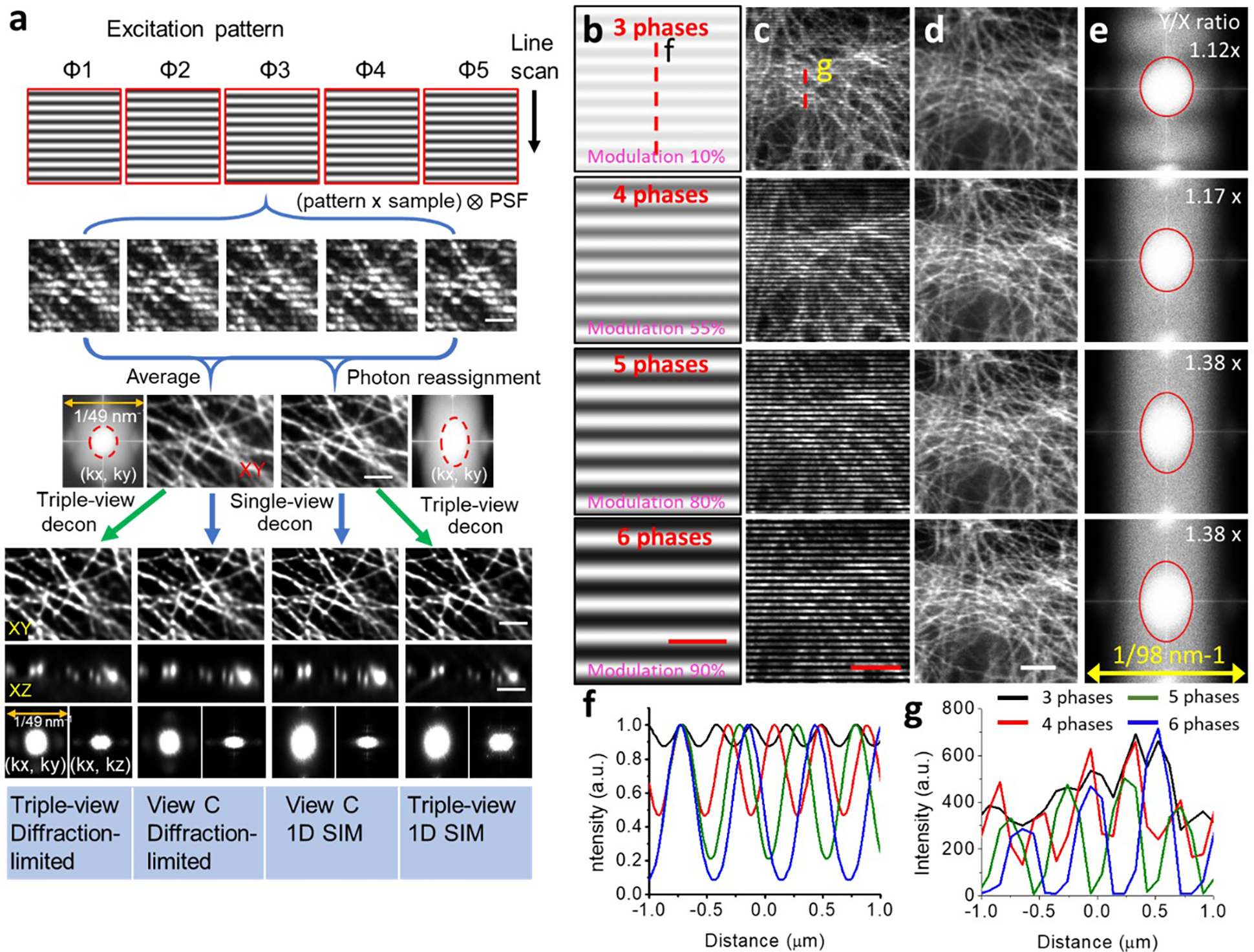
a) Workflow for a single scanning direction and extension for multi-view 1D SIM. Five confocal images are acquired per plane, each with illumination structure shifted 2π/5 in phase relative to the previous position. Averaging produces diffraction-limited images. Detecting each illumination maximum and reassigning the fluorescence signal around it (photon reassignment) improves spatial resolution in the direction of the line scan. Combining image volumes acquired from multiple views further improves volumetric resolution. Images are of immunolabeled microtubules in fixed U2OS cells and corresponding Fourier transforms. Scale bar: 2 μm. b) Simulated fluorescence patterns elicited by (top to bottom) 3, 4, 5, 6 phase illumination. Modulation contrast for each pattern is also indicated. Scale bar: 1 μm. See also Supplementary Methods. c) Raw data as excited with 3, 4, 5, 6 phase illumination. d) Corresponding deconvolved result after photon-reassignment. Scale bars in c-d): 3 μm. e) Fourier transforms corresponding to d). Vertical/horizontal resolution improvement corresponding to red ellipse also indicated. f) Line profiles for 3, 4, 5, 6 phase illumination, corresponding to dotted red line in b). g) As in f) but corresponding to dotted line in c).

Extended Data Fig. 11, Triple-view 1D SIM of C. elegans embryo.

a) Fixed C. elegans embryo (strain DCR6681) with tubulin immunolabeled with α-alpha tubulin primary, α-mouse-biotin, Streptavidin Alexa Fluor 568, imaged via lower View C (left) and triple-view 1D SIM mode (right). Lateral (left) and axial (right) maximum intensity projections are shown in each case. Scale bars: 5 μm. Higher magnification lateral b) views and axial c) views of yellow and red rectangular regions in a) are also indicated, highlighting progressive improvement in resolution from view C (left), to triple-view diffraction-limited result (middle), to triple-view 1D SIM result (right). Scale bars: 2 μm.

Extended Data Fig. 12, Triple-view 1D SIM of cells.

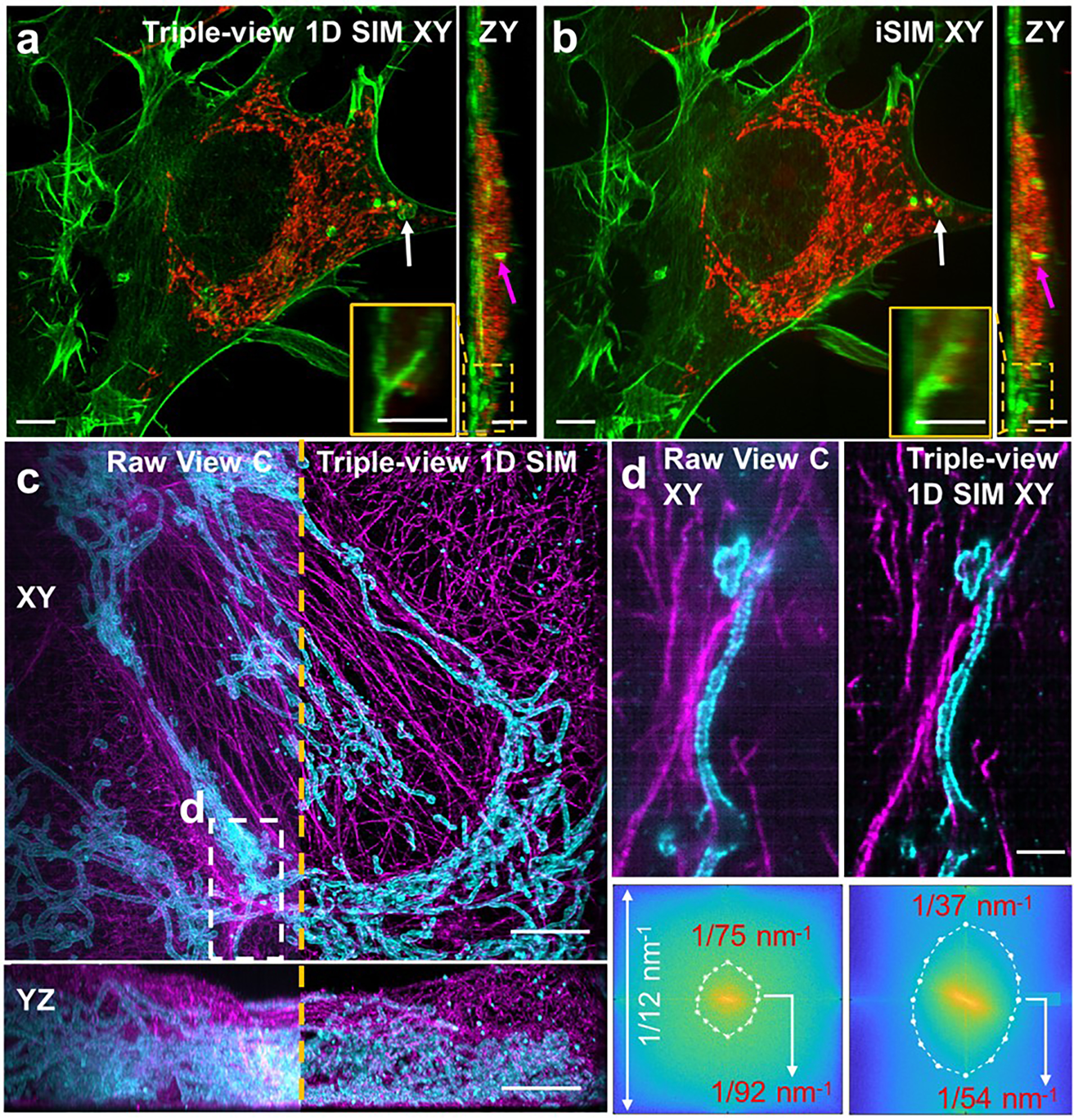
a, b) Comparative triple-view SIM a) and instant SIM b) maximum intensity projections of the same fixed HEY-T30 cell embedded in collagen gel, labeled with MitoTracker Red CMXRos and Alexa Fluor 488 phalloidin. White and magenta arrows: the same features in lateral (left) and axial (right) projections. Insets are higher magnification axial views of dashed rectangular regions. c) Comparative raw single view C (left of dashed orange line) and triple-view SIM (right of dashed line) maximum intensity projections of fixed and 4x expanded U2OS cell, immunolabeled with rabbit anti-Tomm20 primary, anti-rabbit-biotin, streptavidin Alexa Fluor 488 marking mitochondria (cyan) and mouse anti-alpha tubulin primary, anti-mouse JF 549, marking tubulin. Lateral (top) and axial (bottom) views are shown. d) Higher magnification views of white dashed region in c), comparing triple-view (left) and triple-view SIM (right) reconstructions. Bottom: sector-based decorrelation analysis to estimate spatial resolution in images at top. Resolution values for horizontal and vertical directions are indicated. Scale bars: a-c) 5 μm, d) 1 μm.

Extended Data Fig. 13, Expansion workflow and imaging results for C. elegans embryos, related to Fig. 3d.

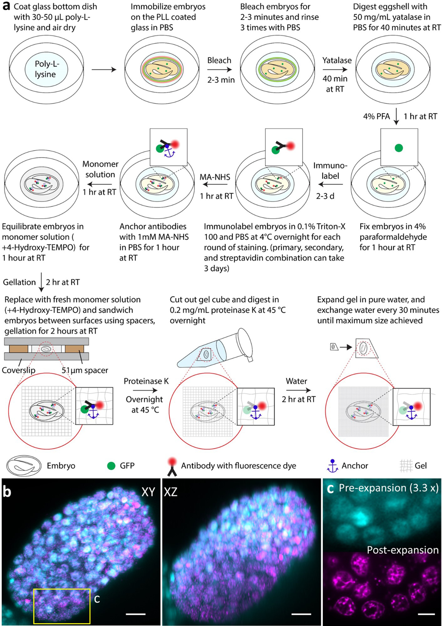
a) Immobilization, permeabilization, fixation, immunostaining, and expansion takes approximately four days. b) Overlay of embryo stained with DAPI before and after expansion after 12-degree affine registration (cyan: pre-expansion; magenta: post-expansion). The embryo was imaged with diSPIM. Single-view maximum intensity projection along XY and XZ views are shown for comparison. The registration results from 7 embryos (normalized cross correlation: 0.72±0.03) show that the expansion factor for whole embryos is 3.29±0.14, with nearly isotropic expansion (3.24±0.14, 3.39±0.14, 3.26±0.17 for x, y and z dimensions, respectively). Scale bar: 5 μm in pre-expansion units. c) Magnified view of the rectangle shown in b), showing no obvious local distortions in nuclei shape during expansion. Scale bar: 2 μm in pre-expansion units.

Extended Data Fig. 14, Simulation of the deep learning method for isotropic in-plane super-resolution imaging.

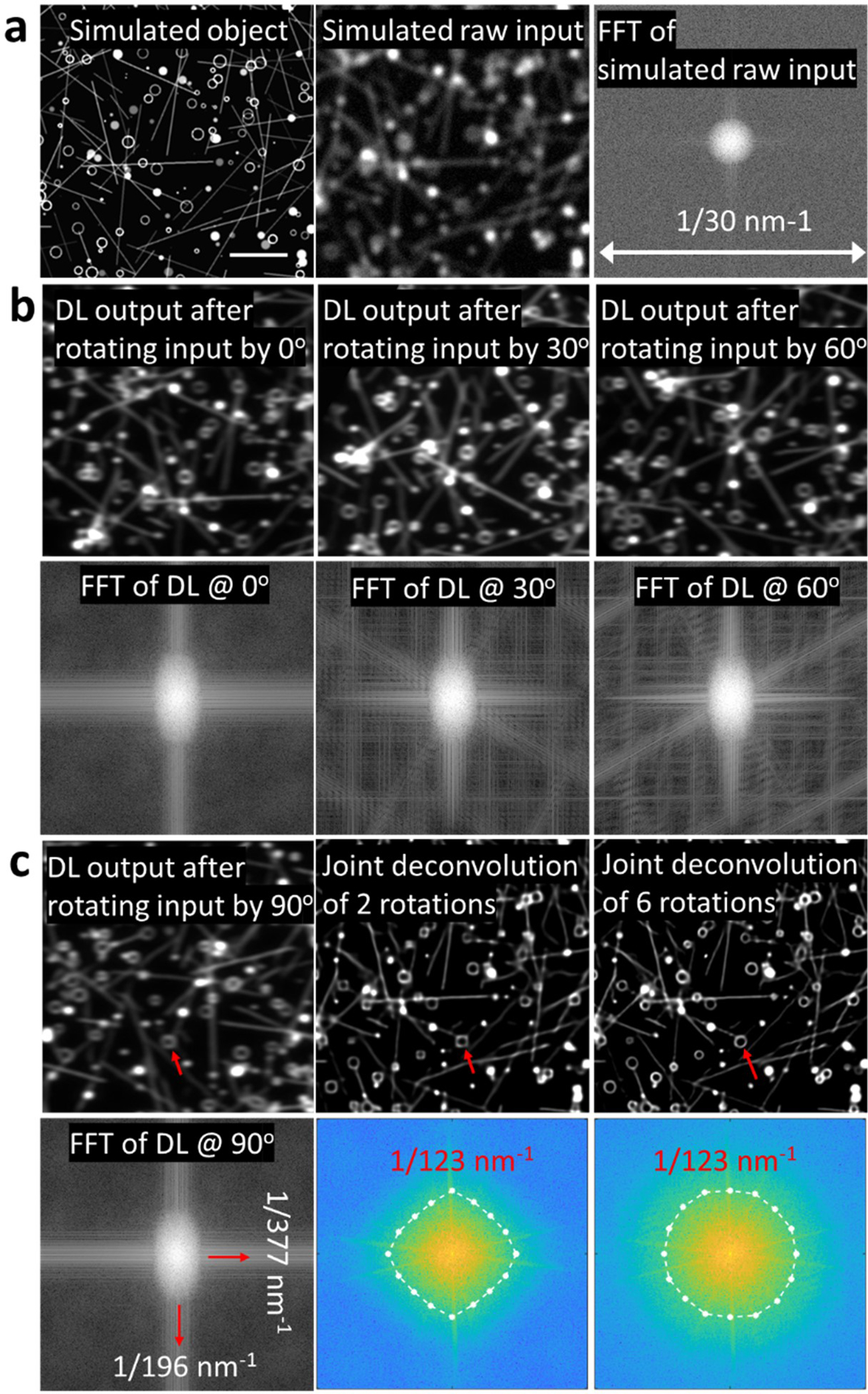
a) An object (left column) consisting of lines and hollow spheres can be blurred to resemble diffraction-limited confocal input (middle column). Fourier transform of the raw input is shown (right column). b) Deep learning 1D super-resolution output with no rotation (left column); deep learning output after rotating input by 30 degrees (middle column); deep learning output after rotating input by 60 degrees (right column). Fourier transforms in bottom row confirm 1D resolution enhancement regardless of rotation angle. c) Deep learning output after rotating input by 90 degrees (left column); outputs after deep learning and joint deconvolution of two orientations (middle column), or six orientations (right column) show progressive improvement in resolution isotropy (red arrows), confirmed with Fourier transforms of the images (bottom row). Ellipses bound decorrelation estimates of resolution (numerical values from ellipse boundary indicated in red text). Scale bar: 2 μm.

Extended Data Fig. 15, Isotropic in-plane super-resolution imaging of fixed cells.

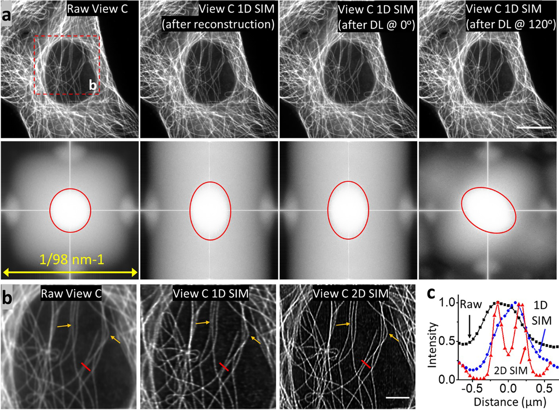
a) Immunolabeled microtubules in fixed U2OS cells, from the same sample shown in Fig. 4b. Shown are raw input (View C); 1D SIM output after physics-based reconstruction with five images; deep learning 1D super-resolution output after rotation at 0 degrees; deep learning 1D super-resolution output after rotation at 120 degrees and rotation back to the original frame. Scale bar: 10 μm. Accompanying Fourier transforms are shown in bottom row. b) Higher magnification view of red dashed region in a), comparing raw confocal input, 1D SIM output after deep learning and deconvolution, and 2D SIM output after deep learning and joint deconvolution after six rotations. Arrows highlight regions for comparison. c) Profiles along red line in b), comparing the resolution of two filaments in 2D SIM mode (red), 1D SIM mode (blue), and confocal input (black).

Extended Data Fig. 16, Isotropic in-plane super-resolution imaging of living cells.

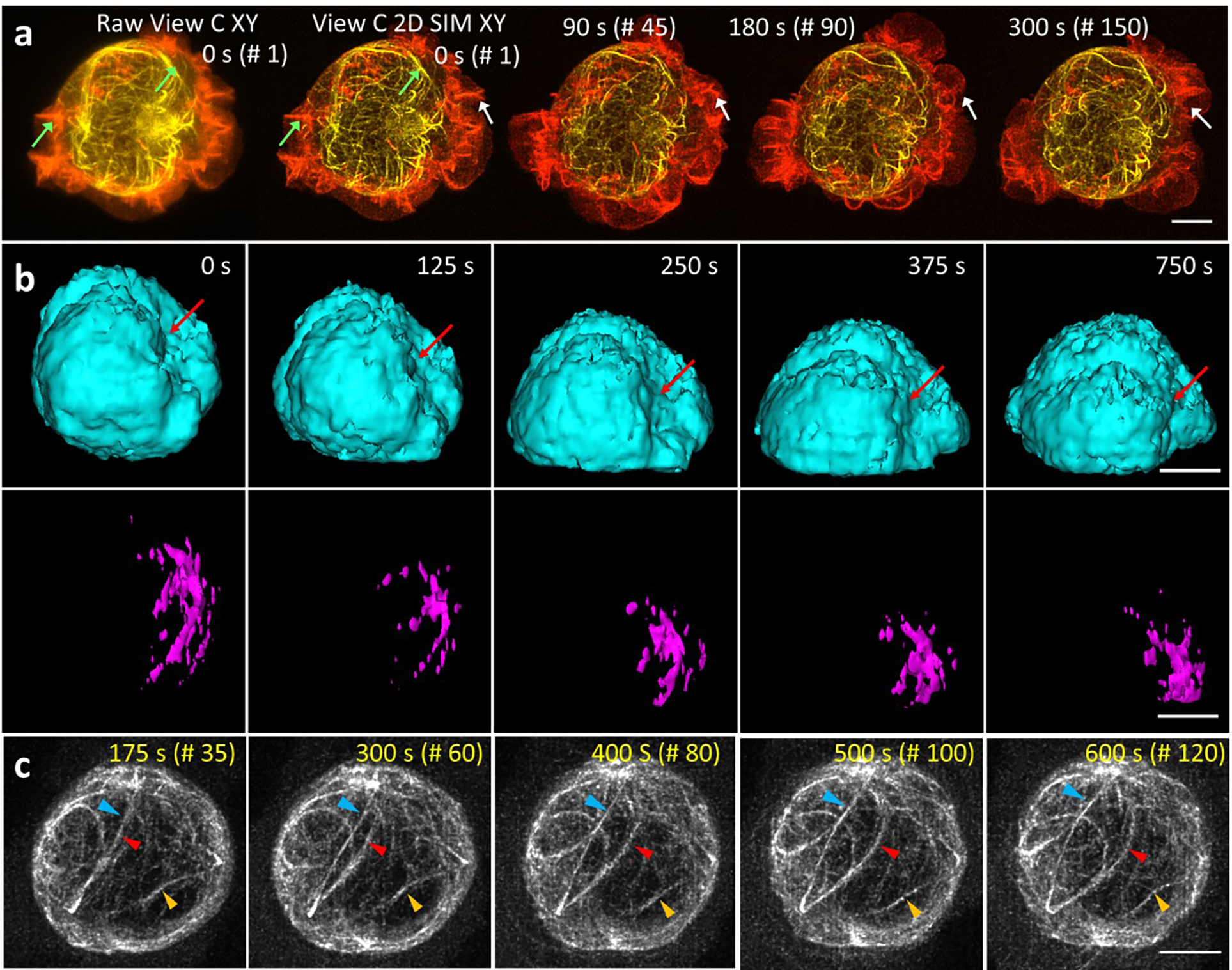
a) Lateral maximum intensity projections of Jurkat T cell expressing EMTB-3XGFP (yellow) and F-tractin-tdTomato (red), volumetrically imaged every 2 s, as imaged with raw line confocal input (View C, left) and 2D SIM output after deep learning and joint deconvolution with six rotations. Four time points from 150 volume series are shown; green arrows highlight features better resolved in 2D SIM output vs. raw input; white arrows indicate actin dynamics at cell periphery. Scale bar: 5 μm. See also Supplementary Video 6. b) Imaris 3D renderings of Jurkat T cell (same sample as shown in Fig. 4c) with nucleus (H2B-GFP, cyan, top) and segmented centrosome (EMTB-mCherry, magenta, bottom) at indicated time points. The centrosome produces a concave nuclear deformation (red arrows), pulling and rotating the nucleus as it becomes docked at the immune synapse. Scale bar: 5 μm. c) Maximum intensity projections over bottom half of EMTB-mCherry volumes at indicated times, showing coordinated movement of the microtubule cytoskeleton. Colored arrowheads mark regions for comparison. See also Supplementary Video 6. Scale bar: 5 μm.

Extended Data Fig. 17, Multi-modality imaging enabled with the multiview line confocal system.

a) Different methods of combining data, enabling a highly versatile imaging platform. Left: Diffraction limited volumes acquired from views A (yellow), B (green), C (red) may be combined with joint deconvolution to yield triple-view diffraction-limited data (RYG arrows). Middle: Alternatively, 5 volumes per view may be collected and processed as in Extended Data Fig. 10 for 1D SIM, and the 3 1D SIM volumes combined using joint deconvolution to reconstruct triple-view 1D SIM data. Right: Instead, confocal data from each view may be passed through 1D SIM networks, and the data combined via joint deconvolution. Combining 6 rotations (for clarity only two are shown in figure) from view C yields View C 2D SIM data. If the procedure is repeated for Views A, B, and the data combined with joint deconvolution, triple-view 2D SIM data may be obtained. XZ cross sections through PSFs are shown in black boxes. Blue volumes are relative sizes of PSFs that result from each process. Scale bars: white: 500 nm, black: 200 nm. b) Applications include wide-field microscopy, single-view line confocal microscopy (from any of the views), single-view 1D SIM, triple-view diffraction limited imaging, and triple-view 1D SIM. With deep learning (red), triple-view line confocal volumes can be predicted from low SNR single-view input, 1D SIM can be predicted from diffraction-limited input, and combination with joint deconvolution allows further extension to single- and triple-view 2D SIM. Biological and imaging performance examples (resolution, imaging speed and duration) are also provided. Resolution values in line confocal microscopy, triple-view line confocal (without deep learning), and triple-view 1D-SIM (without deep learning) are estimated from immunostained microtubules in fixed U2OS cells. Deep learning resolution values are estimated from fine C. elegans embryo neurites (triple-view confocal) or actin fibers (single view 2D SIM, triple-view 2D SIM). See also Supplementary Table 1. c) Decorrelation resolution analysis from the images of worm L4 larval (strain DCR8528) expressing membrane targeted GFP primarily in the nervous system. See also Extended Data Fig. 18d and Fig. 4i–m. Data (mean ± standard deviation) are derived from 45 measurements (3 animals, 15 planes per animal). Given the ~2.3-fold improvement laterally and ~2.6-fold improvement axially, the triple-view 2D SIM (253 × 253 × 322 nm³) result offers a volume resolution improvement of ~13.8-fold over the raw view C data (601 × 561 × 836 nm³). d) Apparent widths (open circles, mean ± standard deviation) of 8 actin fibers from the cell presented in Fig. 4n–q, comparing lateral (left) and axial (right) full width at half maximum in different microscope modalities. Given the ~2.2-fold improvement laterally and ~2.4-fold improvement axially, the triple-view 2D SIM result offers a volume resolution improvement of ~11.6-fold over the raw view C data.

Extended Data Fig. 18, Multiview super-resolution imaging of larval worm.

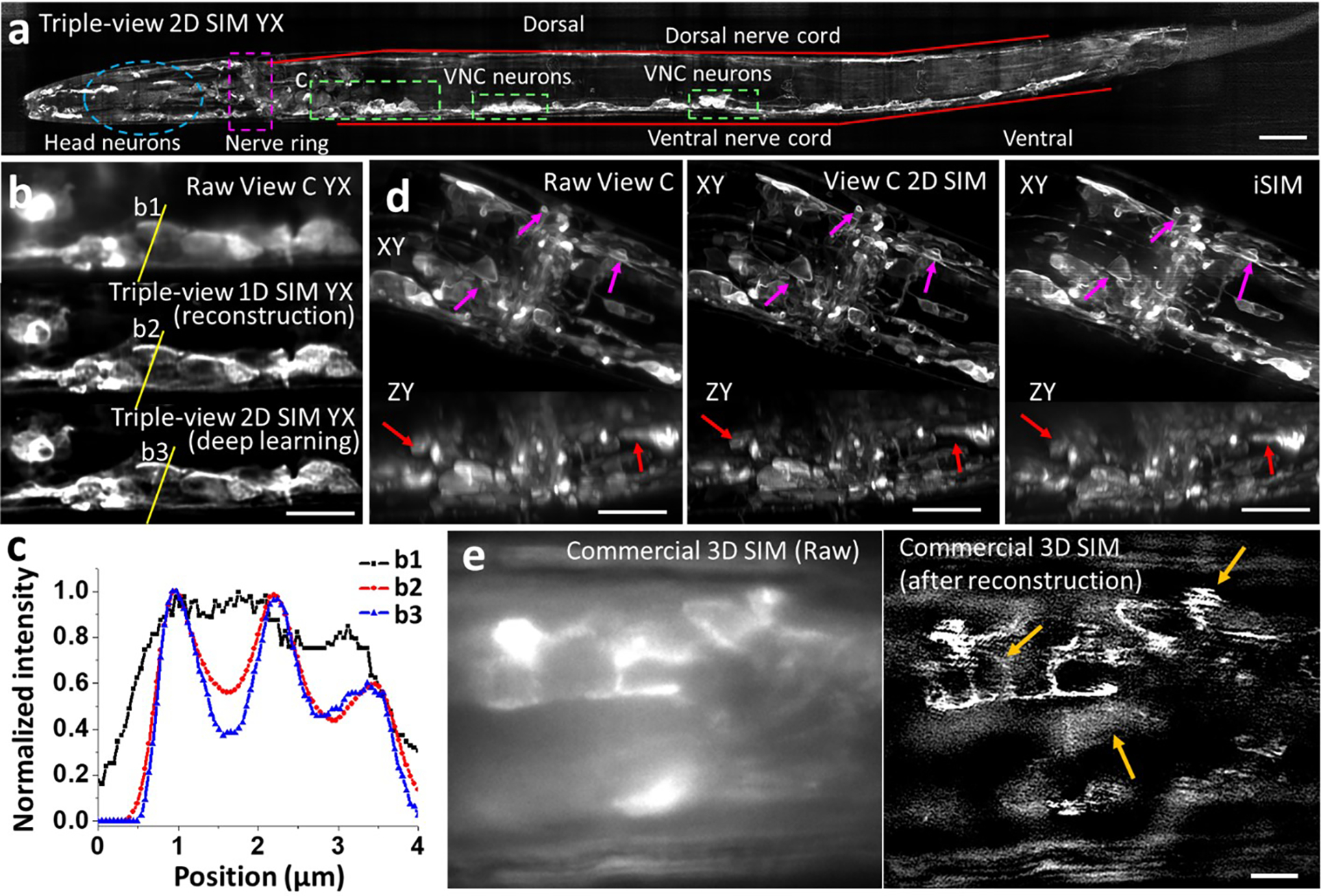
a) Maximum intensity projection of fixed L2 stage larval worm expressing membrane targeted GFP primarily in the nervous system, imaged in triple-view 2D SIM mode. Anatomy as highlighted. b) Higher magnification views (single slices 6 μm into volume) of dashed green rectangle in a), highlighting VNC neurons as viewed in diffraction-limited View C (upper), triple-view 1D SIM obtained by processing 15 volumes (5 per view, middle), and triple-view 2D SIM mode (3 volumes, 1 per view, lower). c) Line profiles corresponding to b1-b3 in b). d) Lateral (upper) and axial (bottom) maximum intensity projections from anesthetized L4 stage larval worm expressing the same marker, comparing dense nerve ring region imaged in diffraction-limited View C (left), View C 2D SIM mode (middle), and iSIM (right). Purple, red arrows highlight labeled cell bodies or membranous protrusions for comparison. See also Fig. 4i–m. e) Fixed C. elegans L2 larvae (strain DCR6681) expressing GFP-membrane marker imaged in commercial OMX 3D SIM system. A single slice ~2 μm from the bottom surface of the worm is shown, derived from 5 μm stack. Raw data (top) and reconstruction (bottom) are shown. No modulation is evident in raw data, and reconstruction shows obvious artifacts (red arrows). Scale bars: a, d) 10 μm; b, e) 5 μm.

Extended Data Table 1, Characterization of imaging field.

Full width at half maximum (FWHM) of illumination (first row) and FWHM derived from images of 100 nm diameter beads in x, y, z direction (latter rows) at different subregions of imaging field (#1 – #9); n = 15 measurements were used to derive means +/− standard deviations for each entry, all units in nm.

	#1	#2	#3	#4	#5	#6	#7	#8	#9
Illummation FWHM	315 ± 23	308 ± 26	313 ± 23	292 ± 30	273 ± 25	289 ± 25	302 ± 16	317 ± 26	293 ± 27
Bead x FWHM	296 ± 23	301 ± 29	314 ± 47	302 ± 27	299 ± 24	310 ± 39	317 ± 68	320 ± 49	308 ± 64
Bead y FWHM	280 ± 25	281 ± 55	293 ± 76	294 ± 45	294 ± 41	283 ± 39	273 ± 79	276 ± 44	291 ± 56
Bead z FWHM	714 ± 97	833 ± 59	789 ± 104	697 ± 125	781 ± 111	700 ± 84	777 ± 137	857 ± 101	831 ± 149

REFERENCES

- 1.Pawley JB Handbook of Biological Confocal Microscopy. Third edn, (Springer Science+Business Media, LLC, 2006). [Google Scholar]
- 2.Laissue PP, Alghamdi RA, Tomancak P & Reynaud EGS, H. Assessing phototoxicity in live fluorescence imaging. Nat Methods 14, 657–661 (2017). [DOI] [PubMed] [Google Scholar]
- 3.Baumgart E & Kubitscheck U Scanned light sheet microscopy with confocal slit detection. Optics Express 20, 21805–21814 (2012). [DOI] [PubMed] [Google Scholar]
- 4.Kumar A et al. Using stage- and slit-scanning to improve contrast and optical sectioning in dual-view inverted light-sheet microscopy (diSPIM). The Biological Bulletin 231, 26–39 (2016). [DOI] [PMC free article] [PubMed] [Google Scholar]
- 5.Guo M et al. Rapid image deconvolution and multiview fusion for optical microscopy. Nature Biotechnol. 38, 1337–1346, doi: 10.1038/s41587-020-0560-x (2020). [DOI] [PMC free article] [PubMed] [Google Scholar]
- 6.Lucy LB An iterative technique for the rectification of observed distributions. Astronomical Journal 79, 745–754 (1974). [Google Scholar]
- 7.Richardson WH Bayesian-Based Iterative Method of Image Restoration. JOSA 62, 55–59 (1972). [Google Scholar]
- 8.Descloux A, Grußmayer KS & Radenovic A Parameter-free image resolution estimation based on decorrelation analysis. Nature Methods 16, 918–924 (2019). [DOI] [PubMed] [Google Scholar]
- 9.Chen F, Tillberg P & Boyden ES Expansion microscopy. Science 347, 543–548 (2015). [DOI] [PMC free article] [PubMed] [Google Scholar]
- 10.He K, Gkioxari G, Dollár P & Girshick R Mask R-CNN. 2017 IEEE conference on Computer Vision (ICCV), 2980–2988 (2017). [Google Scholar]
- 11.Lin T-Y et al. in ECCV 2014 Vol. 8693 (eds Fleet D, Pajdla T, Schiele B, & Tuytelaars T) (Springer, 2014). [Google Scholar]
- 12.Kosmach A et al. Monitoring mitochondrial calcium and metabolism in intact tissues: Application to the beating MCU-KO heart. In review, Nature Methods (2021). [DOI] [PMC free article] [PubMed] [Google Scholar]
- 13.Wu Y et al. Inverted selective plane illumination microscopy (iSPIM) enables coupled cell identity lineaging and neurodevelopmental imaging in Caenorhabditis elegans. Proc. Natl. Acad. Sci. USA 108, 17708–17713 (2011). [DOI] [PMC free article] [PubMed] [Google Scholar]
- 14.Weigert M et al. Content-aware image restoration: pushing the limits of fluorescence microscopy. Nat Methods 15, 1090–1097 (2018). [DOI] [PubMed] [Google Scholar]
- 15.Sulston JE, Schierenberg E, White JG & Thomson JN The embryonic cell lineage of the nematode Caenorhabditis elegans. Dev. Biol 100, 64–119 (1983). [DOI] [PubMed] [Google Scholar]
- 16.Wu Y et al. Spatially isotropic four-dimensional imaging with dual-view plane illumination microscopy. Nat Biotechnol 31, 1032–1038 (2013). [DOI] [PMC free article] [PubMed] [Google Scholar]
- 17.Kumar A et al. Dual-view plane illumination microscopy for rapid and spatially isotropic imaging. Nature Protocols 9, 2555–2573 (2014). [DOI] [PMC free article] [PubMed] [Google Scholar]
- 18.Duncan LH et al. Isotropic light-sheet microscopy and automated cell lineage analyses to catalogue Caenorhabditis elegans embryogenesis with subcellular resolution. J Vis Exp 148, e59533 (2019). [DOI] [PMC free article] [PubMed] [Google Scholar]
- 19.Towlson EK, Vértes PE, Ahnert SE, Schafer WR & Bullmore ET The Rich Club of the C. elegans Neuronal Connectome. Journal of Neuroscience 33, 6380–6387 (2013). [DOI] [PMC free article] [PubMed] [Google Scholar]
- 20.White JG, Southgate E, Thomson JN & Brenner S The Structure of the Nervous System of the Nematode Caenorhabditis elegans. Phil. Trans. R. Soc. London Ser. B 314, 1–340 (1986). [DOI] [PubMed] [Google Scholar]
- 21.Armenti ST, Lohmer LL, Sherwood DR & Nance J Repurposing an endogenous degradation system for rapid and targeted depletion of C. elegans proteins. Development 141, 4640–4647 (2014). [DOI] [PMC free article] [PubMed] [Google Scholar]
- 22.Wu Y & Shroff H Faster, sharper, and deeper: structured illumination microscopy for biological imaging. Nature Methods 15, 1011–1019 (2018). [DOI] [PubMed] [Google Scholar]
- 23.Fischer RS, Gardel ML, Ma X, Adelstein RS & Waterman CM Local cortical tension by myosin II guides 3D endothelial cell branching. Curr Biol. 19, 260–265 (2009). [DOI] [PMC free article] [PubMed] [Google Scholar]
- 24.York AG et al. Instant super-resolution imaging in live cells and embryos via analog image processing. Nat Methods 10, 1122–1126 (2013). [DOI] [PMC free article] [PubMed] [Google Scholar]
- 25.Gambarotto D et al. Imaging cellular ultrastructures using expansion microscopy (U-ExM). Nat Methods 16, 71–74 (2019). [DOI] [PMC free article] [PubMed] [Google Scholar]
- 26.Tabara H, Motohashi T & Kohara Y A Multi-Well Version of in Situ Hybridization on Whole Mount Embryos of Caenorhabditis Elegans. Nucleic Acids Research 24, 2119–2124 (1996). [DOI] [PMC free article] [PubMed] [Google Scholar]
- 27.Chen J et al. Three-dimensional residual channel attention networks denoise and sharpen fluorescence microscopy image volumes. Nature Methods 18, 678–687, doi: 10.1101/2020.08.27.270439 (2020). [DOI] [PubMed] [Google Scholar]
- 28.Wu Y et al. Simultaneous multiview capture and fusion improves spatial resolution in wide-field and light-sheet microscopy. Optica 3, 897–910 (2016). [DOI] [PMC free article] [PubMed] [Google Scholar]
- 29.Barth R, Bystricky K & Shaban HA Coupling chromatin structure and dynamics by live super-resolution imaging. Science Advances 6 (2020). [DOI] [PMC free article] [PubMed] [Google Scholar]
- 30.Han X et al. A polymer index-matched to water enables diverse applications in fluorescence microscopy. Lab Chip 21, 1549–1562 (2021). [DOI] [PMC free article] [PubMed] [Google Scholar]
- 31.Chen BC et al. Lattice light-sheet microscopy: imaging molecules to embryos at high spatiotemporal resolution. Science 346, 1257998 (2014). [DOI] [PMC free article] [PubMed] [Google Scholar]
- 32.Gustafsson MGL et al. Three-Dimensional Resolution Doubling in Wide-Field Fluorescence Microscopy by Structured Illumination. Biophys. J 94, 4957–4970 (2008). [DOI] [PMC free article] [PubMed] [Google Scholar]
- 33.Rego EH et al. Nonlinear structured-illumination microscopy with a photoswitchable protein reveals cellular structures at 50-nm resolution. Proc. Natl. Acad. Sci. USA 109, E135–E143 (2011). [DOI] [PMC free article] [PubMed] [Google Scholar]
- 34.Krüger J-R, Keller-Findeisen J, Geisler C & Egner A Tomographic STED microscopy. Biomed Opt Express 11, 3139–3163 (2020). [DOI] [PMC free article] [PubMed] [Google Scholar]
- 35.Wu Y et al. Reflective imaging improves spatiotemporal resolution and collection efficiency in light sheet microscopy. Nat Commun. 8, 1452 (2017). [DOI] [PMC free article] [PubMed] [Google Scholar]
- 36.Shroff H, York A, Giannini JP & Kumar A Resolution enhancement for line scanning excitation microscopy systems and methods USA patent 10,247,930 (2019).
- 37.Wang H et al. Deep learning enables cross-modality super-resolution in fluorescence microscopy. Nat Methods 16, 103–110 (2019). [DOI] [PMC free article] [PubMed] [Google Scholar]
- 38.Ji N Adaptive optical fluorescence microscopy. Nature Methods 14, 374 (2017). [DOI] [PubMed] [Google Scholar]
- 39.Royer LA et al. Adaptive light-sheet microscopy for long-term, high-resolution imaging in live organisms. Nat Biotechnol. 34, 1267–1278 (2016). [DOI] [PubMed] [Google Scholar]
- 40.Liu T-L et al. Observing the cell in its native state: Imaging subcellular dynamics in multicellular organisms. Science 360, eaaq1392 (2018). [DOI] [PMC free article] [PubMed] [Google Scholar]
- 41.Zheng W et al. Adaptive optics improves multiphoton super-resolution imaging. Nat Methods 14, 869–872 (2017). [DOI] [PMC free article] [PubMed] [Google Scholar]
Associated Data
This section collects any data citations, data availability statements, or supplementary materials included in this article.
Supplementary Materials
Data Availability Statement
The data that support the findings of this study are included in the Extended Data Figures and Supplementary Videos, with some representative source data for the main figures (Figs, 1c, 1g, 2a, 2h, 3b, 4b, 4i). publicly available at https://zenodo.org/record/5495955#.YVItPTHMJaS. Other datasets are available from the corresponding author upon reasonable request.