Perfusion Imaging: An Advection Diffusion Approach

Abstract

Perfusion imaging is of great clinical importance and is used to assess a wide range of diseases including strokes and brain tumors. Commonly used approaches for the quantitative analysis of perfusion images are based on measuring the effect of a contrast agent moving through blood vessels and into tissue. Contrast-agent free approaches, for example, based on intravoxel incoherent motion and arterial spin labeling, also exist, but are so far not routinely used clinically. Existing contrast-agent-dependent methods typically rely on the estimation of the arterial input function (AIF) to approximately model tissue perfusion. These approaches neglect spatial dependencies. Further, as reliably estimating the AIF is non-trivial, different AIF estimates may lead to different perfusion measures. In this work we therefore propose PIANO, an approach that provides additional insights into the perfusion process. PIANO estimates the velocity and diffusion fields of an advection-diffusion model best explaining the contrast dynamics without using an AIF. PIANO accounts for spatial dependencies and neither requires estimating the AIF nor relies on a particular contrast agent bolus shape. Specifically, we propose a convenient parameterization of the estimation problem, a numerical estimation approach, and extensively evaluate PIANO. Simulation experiments show the robustness and effectiveness of PIANO, along with its ability to distinguish between advection and diffusion. We further apply PIANO on a public brain magnetic resonance (MR) perfusion dataset of acute stroke patients, and demonstrate that PIANO can successfully resolve velocity and diffusion field ambiguities and results in sensitive measures for the assessment of stroke, comparing favorably to conventional measures of perfusion.

I. Introduction

The goal of perfusion imaging (PI) is to quantify blood flow through the brain parenchyma by serial imaging. Widely-used perfusion measurement techniques include injecting an intravascular tracer (e.g., in CT perfusion, Dynamic Susceptibility Contrast-enhanced (DSC) and Dynamic Contrast-Enhanced (DCE) MR perfusion) [?], using magnetically-labeled arterial blood water protons as an endogenous tracer (Arterial spin labeling (ASL)) [?], or using positron emission tomography (PET) [?]. The resulting quantitative measures help clinical diagnosis and clinical decision-making, for example, to assess acute strokes and brain tumors. These measures also help to facilitate individualized treatment of stroke patients based on brain tissue status [?]. Despite its benefits, the widespread use of PI still faces many challenges. At present, the mainstream approach for postprocessing PI source data, a time series of 3D volumetric images, is using tracer kinetic models to estimate hemodynamic parameters for each voxel. This then results in 3D perfusion parameter maps [?]. Specifically, an arterial input function (AIF) is selected to approximate the delivery of intravascular tracer to tissue. Perfusion parameter maps are then computed based on the AIF and the observed concentration of contrast agent (CA) at each voxel by a deconvolution algorithm [?]. However, there exist substantial differences in perfusion parameter maps generated across institutions, mainly caused by different AIF selection procedures, deconvolution techniques, and interpretations of perfusion parameters [?], [?], [?].

Moreover, postprocessing approaches for PI are performed on individual voxels, thereby disregarding spatial dependencies of contrast dynamics. Some efforts exist to fit CA transport via partial differential equations (PDEs) [?], [?], [?]. However, these approaches ultimately reduce to voxel-based analyses – parameters of a closed-form solution of the associated PDEs are estimated to fit the concentration time-curve voxel-by-voxel. The work by Cookson et al. [?] is most closely related to our proposed approach. In this work, advection-diffusion PDEs are used to model CA transport within cerebral blood vessels and brain tissue. However, it is assumed that both velocity and diffusion are constant over the entire domain, which is unrealistic in real tissue. In fact, the spatially varying nature of perfusion is, for example, precisely the critical aspect of stroke assessment. As a result of the constancy assumption only simulations are considered in [?], but estimations based on real data are not explored.

Contributions:

We therefore propose Perfusion Imaging via AdvectioN-diffusiOn (PIANO), an approach which models CA transport by a variable-coefficient advection-diffusion PDE. To the best of our knowledge, PIANO is the first PI work taking the spatial relations between voxels into account. Specifically, given a time series of CA concentration 3D images, PIANO estimates spatially-varying velocity and diffusion fields of the advection-diffusion model that best explains CA passage. By physically modeling CA transport via advection and diffusion, PIANO does not require AIF selection or deconvolution algorithms to compute perfusion parameter maps, which are required in conventional PI postprocessing approaches and may yield differences in parameter map estimations. We extensively assess the estimation behavior of PIANO. In particular, we assess PIANO’s ability to disentangle velocity from diffusion estimates and its robustness to noise. We further apply PIANO on a public brain MR perfusion dataset of acute stroke patients. Quantitative comparisons demonstrate the advantage of PIANO feature maps over conventional perfusion parameter maps. We describe and test PIANO in the context of brain PI. The approach, however, is general and could conceivably be applied to other PI approaches, e.g., CT perfusion, as well as PI in other organs, e.g., heart, lung, liver.

This manuscript is a significant extension of our work: Peirong Liu, Yueh Z. Lee, Stephen R. Aylward and Marc Niethammer, “PIANO: Perfusion Imaging via Advection-diffusion”: In 23rd International Conference on Medical Image Computing and Computer Assisted Intervention (MIC-CAI), 2020. Specifically, in this work, we provide detailed experimental evaluations from multiple aspects: (1) We show that the velocity and diffusion fields estimated by PIANO fall within reasonable value ranges that are consistent with value ranges reported in literature; (2) We demonstrate the effectiveness and robustness of PIANO, by exploring its robustness to noise; (3) We further verify the capability of PIANO to disentangle the estimation of advection velocities from the estimation of the diffusion process.

II. Perfusion Imaging via Advection-diffusion (PIANO)

First, Sec ?? describes how we model CA transport as a combination of advection and diffusion. Sec. ?? then discusses how PIANO estimates the velocity and the diffusion fields that best explain the contrast dynamics.

A. Governing Equations

After the injected CA has fully flowed into the brain, the observed local changes of CA concentration (which we refer to as concentration in what follows) in the brain can generally be explained by two dominating macroscopic effects: advection and diffusion. Advection mainly describes the transport of CA driven by the blood flow within the blood vessels, while diffusion captures the movements of freely-diffusive CA within capillaries and the macroscopic effect of capillary transport. Note that because the voxel size in PI (≈ 1 mm) is orders of magnitude larger than the capillary radii [?], capillary blood transport may manifest as diffusion macroscopically. In general, the diffusion term in this manuscript should be considered a combination of all these effects at voxel scale.

Alg. 1:

Pseudo-code for PIANO

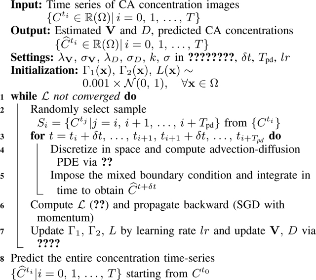T_pd: the number of consecutive time points in one training sample; Convergence criterion: |$\mathcal{L}$ of current iteration – $\mathcal{L}$ of last iteration|/$\mathcal{L}$ of last iteration < 0.001 for 10 subsequent iterations.

Let C(x, t) denote the concentration at location x in the brain $\mathrm{\Omega }\subset {ℝ}^3$, at time t. Local concentration may be modeled as an advection-diffusion equation:

$$\frac{\partial C(\mathbf{x},t)}{\partial t}=-\nabla \cdot (\mathbf{V}(\mathbf{x})C(\mathbf{x},t))+\nabla \cdot (D(\mathbf{x})\nabla C(\mathbf{x},t)),$$ (1)

where V(x) = (V^x(x), V^y(x), V^z(x))^T is the spatially-varying velocity, with each component referring to the blood flow velocity in directions x, y, z respectively. D is a spatially-varying (non-negative) diffusion scalar field governing CA diffusion¹. We assume V and D to be constant in time to simplify our estimation problem². Further, assuming the blood flow is incompressible everywhere, i.e., V is divergence-free (∇ · V(x) = 0, ∀x ∈ Ω), ?? can be simplified to:

$$\frac{\partial C(\mathbf{x},t)}{\partial t}=-\mathbf{V}(\mathbf{x})\cdot \nabla C(\mathbf{x},t)+\nabla \cdot (D(\mathbf{x})\nabla C(\mathbf{x},t)).$$ (2)

B. Estimating Advection and Diffusion

Sec. ?? described PIANO’s advection-diffusion model for CA transport. Here, we focus on a particular approach to estimate divergence-free vector fields V and non-negative diffusion scalar fields D from time series of measured 3D volumetric concentration images, $\left\{{\left(C^{t_i}\right)}_{N_x\times N_y\times N_z}\in ℝ(\mathrm{\Omega })\mid i=0,1,\dots ,T\right\}$, with temporal resolution Δt.

1). Parametrization of Velocity and Diffusion Fields:

To ensure that the vector field V is divergence-free, we represent it by two scalar fields Γ₁, Γ₂ [?]:

$$\mathbf{V}(\mathbf{x})=\nabla {\mathrm{\Gamma }}_1(\mathbf{x})\wedge \nabla {\mathrm{\Gamma }}_2(\mathbf{x}),{\mathrm{\Gamma }}_1,{\mathrm{\Gamma }}_2\in ℝ(\mathrm{\Omega }),\forall \mathbf{x}\in \mathrm{\Omega },$$ (3)

where ∧ denotes the exterior product between vectors in ${ℝ}^3$. To construct a non-negative scalar field, we parametrize D as:

$$D(\mathbf{x})=L^2(\mathbf{x}),L\in ℝ(\mathrm{\Omega }),\forall \mathbf{x}\in \mathrm{\Omega }.$$ (4)

2). Numerical Flow:

The voxel spacings δx, δy, δz of the given 3D volumetric concentration images naturally introduce corresponding grid sizes in axial, coronal and sagittal directions. We use a first-order upwind scheme [?] to approximate the partial differential operators of the advection term in ??, and nested forward-backward differences for the diffusion term: forward differences for ∇· and backward differences for ∇C in ??. Discretizing all spatial derivatives on the right hand side of ?? results in a system of ordinary differential equations, which we solve by numerical integration. Specifically, we impose mixed boundary conditions (BCs) on the system: Dirichlet BCs are applied on the first and last axial slices³ which simply specify the measured concentrations. By applying these BCs, we assume the inflow from and the outflow to the out-of-brain domains are reflected by the CA’s concentration on these two axial slices across the observed time points. We impose homogeneous Neumann BCs on the outer brain contours in the remaining axial slices, assuming no contrast agent passes through these boundaries. We use the Runge-Kutta 45 (RK45) method to integrate the advection-diffusion equation in time (Δt). Hence, this allows us to predict ${\widehat{C}}^{t+\delta t}$. Note that the chosen δt is typically smaller than the temporal resolution of the given concentration time series images (δt), to satisfy the Courant-Friedrichs-Lewy (CFL) condition [?]. This is required to ensure numerical stability.

3). Estimation:

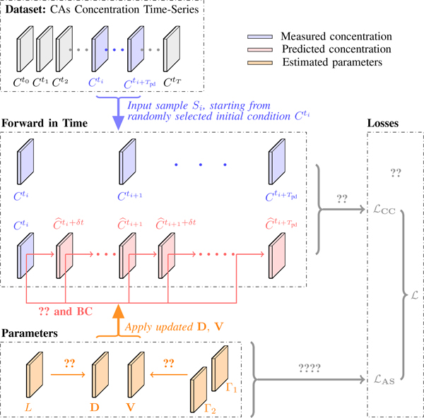
Given an initial state C^t, PIANO applies the current estimate of V, D to C^t by ?? and predicts subsequent concentration images with time step δt. Instead of starting from a specific concentration image, we randomly pick an image from the given concentration time series as the initial condition for each estimating iteration. We then integrate the PIANO model forward to time frame T_pd (Fig. ??). This reduces the sensitivity of the estimated V and D to varying initial conditions. We define our estimation losses as follows.

1. Collocation Concentration Loss.: Given a sample $\left\{C^{t_i}\in ℝ(\mathrm{\Omega })\mid i=0,1,\dots ,T_{\text{pd}}\right\}$, with $t_0,t_1,\dots ,t_{T_{\text{pd}}}$ as collocation points, we define the collocation concentration loss $\left({\mathcal{L}}_{CC}\right)$ as the mean squared error of the predicted concentrations at $t_1,\dots ,t_{T_{\text{pd}}}$. This encourages estimates to be close to the measurements:

   $${\mathcal{L}}_{CC}=\frac{1}{T_{\text{pd}}}\sum _{i=1}^{T_{\text{pd}}}\frac{1}{\left|\mathrm{\Omega }\right|}{\int }_{\mathrm{\Omega }}{(C^{t_i}(\mathbf{x})-{\widehat{C}}^{t_i}(\mathbf{x}))}^{2}d\mathbf{x}\text{.}$$ (5)
2. Anisotropic Smoothness Regularizations.: Assuming the estimated fields are spatially smooth, we impose regularization terms on ∇V, ∇D as

   $$\{\begin{array}{l}{\mathcal{L}}_{A{S}_{\mathbf{V}}}=\sum _{i\in \{x,y,z\}}\frac{1}{\left|\mathrm{\Omega }\right|}{\int }_{\mathrm{\Omega }}{w}_{\mathbf{V}}{\Vert \nabla V^i\Vert }_2^{2}d\mathbf{x},\hfill \\ {\mathcal{L}}_{A{S}_D}=\frac{1}{\left|\mathrm{\Omega }\right|}{\int }_{\mathrm{\Omega }}{w}_D\Vert \nabla D{\Vert }_2^{2}d\mathbf{x},\hfill \end{array}$$ (6)

   where the associated coefficients w_V, w_D are computed as

   $$\{\begin{array}{l}{w}_{\mathbf{V}}=\sum _{i\in \{x,y,z\}}\frac{g({\Vert \nabla (K_{\sigma }\ast V^i)\Vert }_2^2)}{3},\hfill \\ w_D=g({\Vert \nabla (K_{\sigma }*D)\Vert }_2^2),\sigma >0,\hfill \end{array}$$ (7)

   with g(s) = exp(−s/k) (k > 0). The decreasing function g is added to reduce the gradient penalty on those regions which have a large likelihood to be edges [?]. To make the estimation relatively insensitive to noise, Gaussian smoothing (K_σ) is applied to the parameter fields first. To avoid the undesirable effect that edges might be formed at different locations for different velocity channels, we average over axes to obtain a common coefficient w_V at each location [?].

Overall, PIANO estimates V, D by minimizing the following sum of losses:

$$\underset{\mathbf{V},D}{\min }\mathcal{L}={\mathcal{L}}_{CC}+{\lambda }_{\mathbf{V}}{\mathcal{L}}_{A{S}_{\mathbf{V}}}+{\lambda }_D{\mathcal{L}}_{A{S}_D},{\lambda }_{\mathbf{V}},{\lambda }_D>0.$$ (8)

III. Dataset Description

In Secs. ??-??, we will test PIANO on both simulated advection-diffusion time-series images for validation purposes (Sec. ??) and real MR perfusion images for practical demonstration (Sec. ??), based on the Ischemic Stroke Lesion Segmentation (ISLES) 2017 ( [?], [?]) dataset. ISLES 2017 dataset includes images for 43 ischemic stroke patients. Each patient has the following images: an apparent diffusion coefficient (ADC) map, a 4D dynamic susceptibility contrast (DSC) MR perfusion image (from 40 to 80 available time points; temporal resolution ≈ 1 s) [?], and a segmented lesion map viewed as the gold-standard lesion. For each patient the dataset also includes five perfusion summary maps: (1) Cerebral blood flow (CBF); (2) Cerebral blood volume (CBV); (3) Mean transit time (MTT); (4) Time to peak (TTP); and (5) Time to peak for the deconvolved residue function (Tmax). In this work, we focus on the ADC map and perfusion parameter maps which correspond to physical measures, i.e., CBF, CBV, MTT, TTP and Tmax, for further quantitative comparison.

We first convert DSC MR perfusion images to concentration images using the relation between the MR signal and CA concentration [?]. Specifically, the concentration can be determined as follows:

$$C\left(\mathbf{x},t_i\right)=-\frac{k_{\text{mr}}}{\text{TE}}\ln \left(\frac{S\left(\text{x},t_i\right)}{S_0}\right),i=1,\dots ,T,$$ (9)

where C(x, t_i), S(x, t_i) denote the CA concentration value and the received MR signal at voxel position x and time t_i, respectively. $\frac{k_{\text{mr}}}{\text{TE}}$ is a constant of proportionality related to the image acquisition process, which is usually set to 1 for the sake of simplicity [?]. The baseline value S₀ is obtained by the mean of S(x, t_j) during the B acquired time frames before the CA bolus arrival:

$$S_0=\frac{1}{B}\sum _{j=1}^{B}S\left(\mathbf{x},t_j\right).$$ (10)

The original perfusion images are typically anisotropic, with a much larger voxel size along the axial (6.5 mm) than in the other two directions (1.2 mm). To obtain a more uniform computational grid for the model, we upsample each concentration image along the axial direction (to 1.3 mm grid size) using the Lanczos Windowed Sinc method [?]. Then we create a concentration time-series dataset for each patient $N:\left\{C^{t_i}\in ℝ(\mathrm{\Omega })\mid i=0,1,\dots ,T_N\right\}$, starting from the time when the total concentration over the entire brain reaches its maximum, at which we assume the CA has been fully transported into the brain, till the last available time point.

IV. Property Validation

Mathematically, PIANO aims at recovering the velocity and diffusion fields of an advection-diffusion process following ??. From a validation point of view, the challenge is that we do not know the ground truth measurements of V and D driving the contrast agent transport for our real data. Therefore, before applying PIANO on real data, in this section, we first validate its three essential properties. We use simulated data where the ground truth V, D is known by construction. Specifically, we assess (1) Effectiveness: the accuracy of the estimated velocity and diffusion fields. I.e., given a time-series of images capturing an advection process, driven by a certain velocity field, is PIANO capable of recovering the underlying velocity field? Similarly, can PIANO successfully recover a diffusion field governing a diffusion process. (2) Robustness: the robustness of PIANO’s estimation to noise. I.e., if measurement errors exist in the given time-series of concentration images, can PIANO still achieve reasonable estimates? (3) Identifiability: does PIANO confuse advection with diffusion, resulting in an incorrect estimation for the underlying velocity (or diffusion) field?

A. PIANO Effectiveness and Robustness Testing

1). Advection Imaging via Advection:

Our goal here is to determine if PIANO can estimate a known velocity field from a concentration time-series consistent with this velocity field. To this end, for each patient in the ISLES 2017 training set, we treat the velocity field estimated by PIANO as the ground truth velocity field (V^gt), and the first image in the concentration time-series dataset $\left\{C^{t_i}\right\}$ (as described in Sec. ??) is used as the initial condition (C⁰). We then simulate ‘advection imaging’ $\left\{C^{t_i}\in ℝ(\mathrm{\Omega })\mid i=0,1,\dots ,40\right\}$, i.e., we create a time-series of concentration images driven by the velocity V := V^gt only via the advection PDE:

$$\frac{\partial C(\mathbf{x},t)}{\partial t}=-\mathbf{V}(\mathbf{x})\cdot \nabla C(\mathbf{x},t).$$ (11)

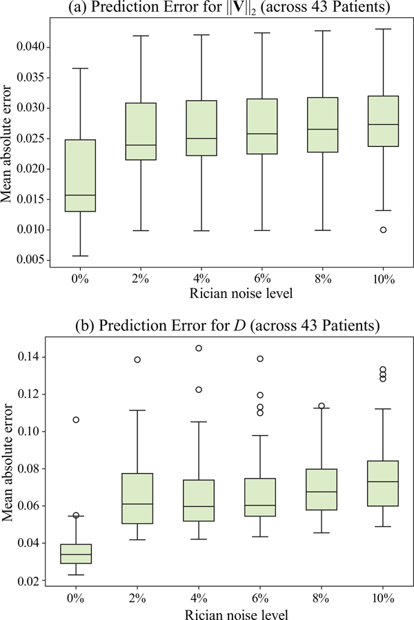
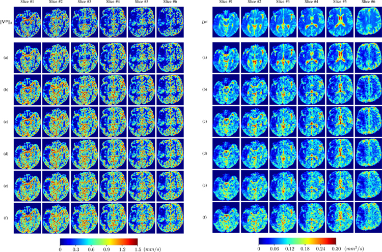
We further simulate noisy concentrations by adding Rician noise [?] with variances equalling 2%, 4%, 6%, 8%, 10% of the originally simulated concentrations $\left\{C^{t_i}\right\}$. We then test how well PIANO can estimate the underlying velocity field via ?? with the same model settings (except without estimating the diffusion) as in Sec. ?? given the original and the noisy concentration time-series. Fig. ?? shows the estimated ‖V^est‖₂ for one patient. Fig. ?? (a) shows the summarized estimation results for all 43 patients. PIANO almost perfectly captures the underlying velocity field, and maintains excellent performance even when estimating from concentrations with varying noise levels.

2). Diffusion Imaging via Diffusion:

Similarly, starting from the same initial condition C⁰ as in the ‘Advection Imaging’ experiment for each patient, we simulate concentration time-series $\left\{C^{t_i}\in ℝ(\mathrm{\Omega })\mid i=0,1,\dots ,40\right\}$ via a diffusion PDE, where we define the ground truth diffusivity D := D^gt via the ADC map of the ISLES 2017 training set (ADC values are scaled by 0.00001 to ensure numerical stability):

$$\frac{\partial C(\mathbf{x},t)}{\partial t}=\nabla \cdot (D(\mathbf{x})\nabla C(\mathbf{x},t)).$$ (12)

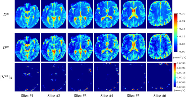
Note that for the simulated data for our numerical experiments, our goal is to obtain non-trivial diffusion fields for our 3D diffusion simulation. We use the ADC map to this end. While this will indeed result in non-trivial diffusion fields, those will not accurately model overall brain perfusion patterns, because the diffusion we capture in our advection-diffusion formulation from CA signal dynamics is different from the water diffusion which ADC is based on. Nevertheless, using ADC to construct a non-trivial diffusion field is beneficial to assess PIANO’s capability for estimating complex diffusion patterns. Note that while the resulting diffusion patterns will most likely not be globally realistic they do not need to be as they will model realistic local patterns which is what PIANO estimates are based on. We also added 2%, 4%, 6%, 8%, 10% levels of Rician noise to obtain simulations of ‘Diffusion Imaging’. The estimated D^est given concentrations of all noise levels for one patient are shown in Fig. ??, PIANO estimation results for all patients are summarized in Fig. ?? (b). Again, PIANO demonstrates its capability to recover the underlying diffusion field. In Fig. ??, when the noise level is increasing, some noisy patterns indeed appear in the associated D^est. Note that the ground truth diffusivity applied in this simulation experiment is about ten times larger than the diffusivity estimated in reality (Fig. ??, Fig. ??).

B. PIANO Identifiability Testing

We verified in Sec. ?? the capability of PIANO to estimate the underlying velocity field governing an advection process (‘Advection Imaging via Advection’), and the original diffusion field given a diffusion process (‘Diffusion Imaging via Diffusion’), respectively. We now test the identifiability properties of PIANO. Specifically, we let PIANO simultaneously estimate both velocity and diffusion fields given a pure advection (or diffusion) process, and explore if it would confound velocity with diffusion as two different physical values.

1). Advection Imaging via Advection-Diffusion:

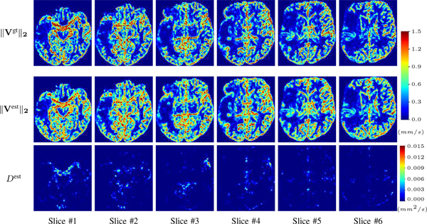
We use the same ‘Advection Imaging’ simulation of Sec. ?? as the concentration dataset for PIANO. However, instead of modeling pure advection (??), we let PIANO estimate both velocity V^est and diffusivity D^est via the advection-diffusion PDE (??) underlying the proposed PIANO model. Fig. ?? shows the estimated ‖V^est‖₂, and D^est fields for one patient. Although PIANO has the freedom to estimate both a velocity and a diffusivity field from pure advection, PIANO differentiates well between advection and diffusion: the estimated ‖V^est‖₂ successfully reproduces the ground truth ‖V^gt‖₂ governing the simulated advection process, just as it already did in the ‘Advection Imaging via Advection’ test (Fig. ??). More importantly, the estimated diffusivity D^est is orders of magnitudes smaller than ‖V^est‖₂, indicating the estimated diffusion is negligible compared to the estimated advection, which is highly consistent with the underlying pure advection of the simulated data.

2). Diffusion Imaging via Advection-Diffusion:

Similarly, we test the behavior of PIANO when estimating both advection and diffusion from a pure diffusion-driven process. The goal is to determine if PIANO is able to recognize that there is only diffusion governing the given concentration time-series. We use the same ‘Diffusion Imaging’ data simulation of Sec. ?? as the concentration dataset, PIANO estimates both velocity V^est and diffusivity D^est. Estimation results in Fig. ?? confirm PIANO’s identifiability again: the estimated ‖V^est‖₂ is almost invisible compared to D^est, even plotted with a 1% value range compared to that for D^est. On the other hand, D^est achieves comparable estimation performance as ‘Diffusion Imaging via Diffusion’ in which PIANO predicts D^est alone (shown in Fig. ??).

V. Experimental Results

In Sec. ?? we validated PIANO based on simulated data. This allowed us to measure errors between the estimated velocity and diffusion fields (V, D) and the ground truth. Our results highlighted the good estimation properties of PIANO. In this Section we apply PIANO to real data, where ground truth measures are not available. We test PIANO on all 43 patients from ISLES 2017 dataset with identical model settings. Specifically, we set λ_V = λ_D = 0.1 (??). In ??, σ = 0.6; k was treated as a ‘noise estimator’ [?], where a histogram of the absolute values of the gradient throughout the current image was computed, and k was set as 90% of the histogram’s integral at every estimating iteration. Throughout the estimation, the prediction temporal resolution is δt = 0.02 s, and $T_{\text{pd}}=\lfloor \frac{T_k}{3}\rfloor$. (See Alg. ??.)

A. PIANO Feature Maps

For a better insight into an estimated velocity field V and diffusion field D, we compute the following maps: (1) V_rgb: Color-coded orientation map of V = (V^x, V^y, V^z)^T, obtained by normalizing V to unit length and mapping its 3 components to red, green, blue respectively; (2) ‖V‖₂: 2 norm of V; (3) D: scalar field in ??.

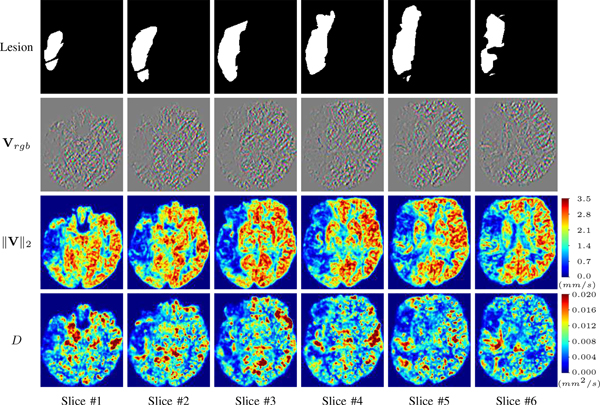
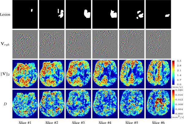
Fig. ?? and Fig. ?? show the PIANO feature maps estimated from two ISLES 2017 patients: all are highly consistent with the lesion in both cases. Details of the blood flow trajectories are revealed in V_rgb by the ridged patterns and the sharp changes of colors in the unaffected (right) hemisphere, while the flat patterns appearing within the lesion provide little directional information about the velocity and indicate low velocity magnitudes. Velocity magnitudes are more directly visualized via ‖V‖₂, from which one can easily locate the lesion where ‖V‖₂ is low. D also indicates lower diffusion values in the lesion, though with less contrast potentially due to the fact that it captures the accumulated effect of CA diffusion at the voxel-level.

B. Predicted CA Concentration

To better illustrate the prediction accuracy, and therefore the estimation accuracy for V and D, of PIANO, we further consider the mean absolute percentage error (MAPE) across all predicted time points:

$$\text{MAPE}=\frac{1}{T_{\text{pd}}}\sum _{i=1}^{T_{\text{pd}}}\left|\frac{C^{t_i}-{\widehat{C}}^{t_i}}{C^{t_i}}\right|,$$ (13)

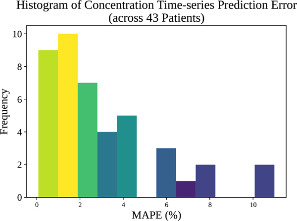
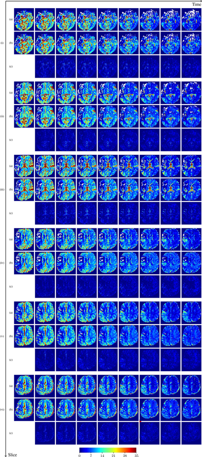
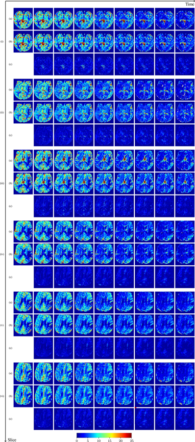
where $C^{t_i}$, ${\widehat{C}}^{t_i}$ denote the observed and predicted CA concentration at t_i, respectively. Averaged over the entire brain for each patient, we compute the histogram of patient-specific MAPE as shown in Fig. ??. In general, the concentration prediction errors are lower than 5% for most patients, and the average MAPE over all 43 patients is 3.06%. This demonstrates PIANO’s capability to predict CA concentration over time. For better visualization, we additionally provide the predicted time-series of CA concentration images and their corresponding MAPE maps in Fig. ?? and Fig. ??. We see that PIANO is capable of predicting the CA concentration given their initial state, indicating its ability to successfully capture V and D. Note that although the concentration values for these two patients differ considerably, caused by the different total volume of injected CA, PIANO is still able to provide plausible estimates.

C. Quantitative Comparison

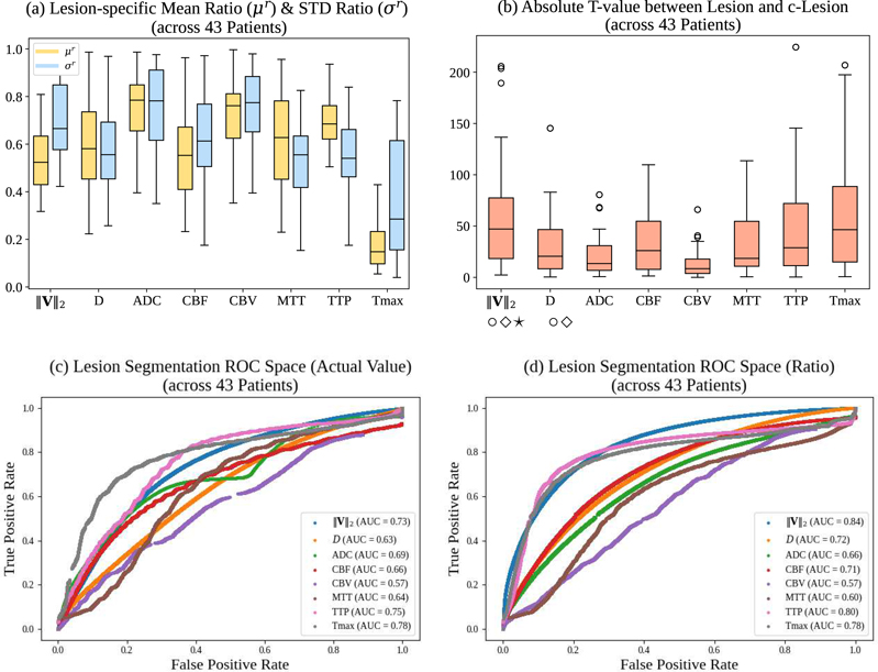
(1) We added comparisons with TTP and Tmax feature maps performance according to R2’s C2 & C10 and R3’s C5. (2) We added quantitative analysis on ROCs of all maps to assess their performances on lesion segmentation according to R1’s C3 and R4’s C14. (3) To avoid potential confusion after adding ROCs comparison, we categorized the three metrics already defined in the original manuscript (μ^r, σ^r, absolute t-value) as “lesion-specific metrics”, and new metrics for lesion segmentation comparisons as “globally-defined metrics”. To quantitatively compare PIANO feature maps with the maps provided by ISLES 2017 in their ability to detect the lesion, we consider the following four metrics for comparison between the different maps.

Lesion-specific metrics:

We first compare feature values in the lesion with the values in the contralateral region of the lesion (c-lesion), where the lesion regions are determined by the lesion segmentations contained in the ISLES 2017 dataset. The c-lesion region is determined by mirroring the lesion segmentation to the unaffected side via the midline of the cerebral hemispheres. Values in the c-lesion then provide a reference for the normal values⁴.

1. Lesion-specific mean ratio (μ^r ∈ [0, 1]): the ratio between the mean values in the lesion and the c-lesion.

   $${\mu }^r=min\left\{\frac{\text{mean}\text{in}\text{lesion}}{\text{mean}\text{in}\text{c-lesion}},\frac{\text{mean}\text{in}\text{c-lesion}}{\text{mean}\text{in}\text{lesion}}\right\};$$ (14)
2. Lesion-specific STD ratio (σ^r ∈ [0, 1]): the ratio between the standard deviation (STD) in the lesion and the c-lesion.

   $${\sigma }^r=min\left\{\frac{\text{STD}\text{in}\text{lesion}}{\text{STD}\text{in}\text{c-lesion}},\frac{\text{STD}\text{in}\text{c-lesion}}{\text{STD}\text{in}\text{lesion}}\right\};$$ (15)

3. Lesion-specific absolute t-value (|t| ≥ 0): the absolute value of the unpaired t-statistic between the values in the lesion and the c-lesion⁵.

Globally-defined metrics:

The three measures above are defined with respect to a given segmented lesion region. Here, we therefore also consider how well the different perfusion maps can distinguish lesion from non-lesion regions. I.e., we want to use them for lesion segmentation. To this end we threshold our maps and compare the resulting segmentations to the segmentations provided by ISLES 2017. Specifically, we compute the receiver operating characteristic (ROC) curves and their associated areas under the curve (AUC).

(4) AUC:

Given a value map to be thresholded for classification, its ROC curve corresponds to the true positive rate (TPR) vs. the false positive rate (FPR) at different classification thresholds, here, for lesion classification. AUC measures the area under the ROC curve, which provides an aggregate measure of performance across all possible classification thresholds and is widely used in evaluations for classification tasks. Here, we explore the following two measures for thresholding and ROC comparisons.

• Actual value. We directly take the values from all maps for ROC and AUC computation.

• Point-wise Ratio. Despite being straightforward, thresholding directly on the actual values for lesion classification is challenging as normal parameter value ranges differ among locations. To sidestep this issue, we further threshold the ratios between the values in the two brain hemispheres. Specifically, we consider the point-wise ratios (r(x)) between left and right hemispheres:

  $$r(\mathbf{x})=\frac{\text{value}\text{at}\mathbf{x}}{\text{value}\text{at}\text{c}-\mathbf{x}},\mathbf{x}\in \mathrm{\Omega },$$ (16)

  where c-x refers to the contralateral position of x via the midline of the cerebral hemispheres. As all our measures are positive, r(x) ≥ 0. Note r(x) is similar to the lesion-specific ratio (μ^r), however, we do not assume any a-priori knowledge of a lesion segmentation for evaluation.

Note that more sophisticated classification methods could be easily applied to PIANO’s feature maps (and all the other feature maps as well) for more accurate lesion segmentation results. We leave this for future work to keep the manuscript focused.

Fig. ?? compares the PIANO and ISLES 2017 maps based on the above four measures computed from all 43 patients. Figs. ??(a-b) show results of lesion-specific measures (μ^r, σ^r, absolute t-value). ‖V‖₂ achieves the highest absolute t-value among all feature maps. Note that even though Tmax achieves a lower (i.e., better) lesion-specific ratio (μ^r) than all other feature maps, its lesion-specific absolute t-value (|t|) is still slightly lower (i.e., worse) than that for ‖V‖₂. On the other hand, Figs. ??(c-d) show ROC comparison results for all maps for lesion segmentation. As lesion segmentation is the goal here the manual lesion segmentations are only used to evaluate the quality of the thresholded segmentations, but are not used to restrict the evaluation region (as for the previous results). When thresholded by the actual values (Fig. ??(c)), Tmax achieves the highest (i.e., best) AUC, and is closely followed by TTP and ‖V‖₂. While using the point-wise ratios (Fig. ??(d)), PIANOS’s ‖V‖₂ outperforms all other maps (including all of the actual value AUCs) and achieves the best segmentation results. This behavior can be explained by realizing that normal values in maps such as ‖V‖₂, D, CBF & CBV, typically vary across space. Hence, using a simple global threshold based on actual values tends to ignore these spatial dependencies, and may therefore lead to misinterpretations of parameter values in normal regions. When using ratios for ROC comparison, one instead considers the relative values between hemispheres. In this way, classification results are less sensitive to actual parameter values even if normal parameter value ranges differ with location. Tab. ?? further summarizes the comparison results over all patients, where PIANO’s feature maps outperform ISLES 2017 maps in 6 of the 11 compared indices. Note also that PIANO maps achieve the best results in every subcategory (i.e., relative mean, relative STD, absolute t-value, and AUC).

D. Cerebral Blood Velocity and Péclet Number

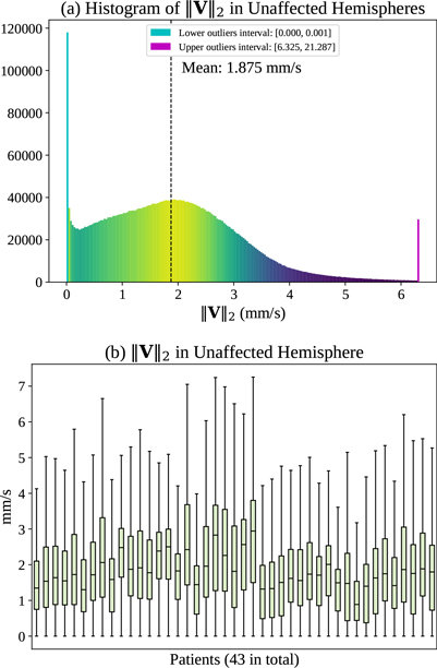
As described in Sec. ??, ‖V‖₂, is the 2 norm of the estimated velocity field V governing the advection process, which describes the transport of CA driven by the cerebral blood flow within the blood vessels. Ivanov et al. [?] provide an in-depth discussion about blood flow velocities in cerebral capillaries. They report a typical range of blood flow velocities between 0.5 to 1.5 mm/s in cerebral capillaries, precapillaries, and arterioles that are not more than 5 μm in luminal diameter. Maximum blood flow velocities in humans can reach up to 100 cm/s in major cerebral arteries such as the middle cerebral arteries (MCAs) [?]. However, such velocities are not observable based on our imaging. Specifically, the V estimated by PIANO, via observing the transport of CA recorded in PI, should be considered as the velocity field averaged over space (with voxel spacing of ≈ 1 mm) and time (with PI temporal resolution of ≈ 1 s). Estimated velocities are therefore significantly lower than the maximum velocities. In fact, mean velocities across a cardiac cycle (V_mean) for cerebral perforating arteries are measured in [?], where the authors report V_mean in the semioval centre (CSO) in the range 0.5–1.0 cm/s, and in the range of 3.9–5.1 cm/s for V_mean in the basal ganglia (BG). Fig. ?? (a) displays the histogram of ‖V‖₂, in the unaffected hemispheres (in which we assume blood flow velocities are in the normal range) of the 43 ISLES 2017 stroke patients. In general, ‖V‖₂ mainly falls within the range of 0–6 mm/s with a mean value of 1.875 mm/s, which is consistent with the cerebral blood flow velocities reported in the above literature. Fig. ?? (b) shows detailed distributions of ‖V‖₂ for each patient. We observe a similar range of ‖V‖₂ for the different patients.

To assess the relation between the estimated advection and diffusion, we resort to the Péclet number (Pe). Pe is a dimensionless number that represents the ratio of the contributions to mass transport by advection to those by diffusion [?]. For mass transfer (i.e., CA in this paper), it is formed as

$$\text{Pe}=\frac{L\Vert \mathbf{V}{\Vert }_2}{D},$$ (17)

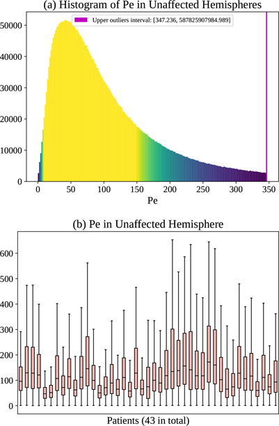
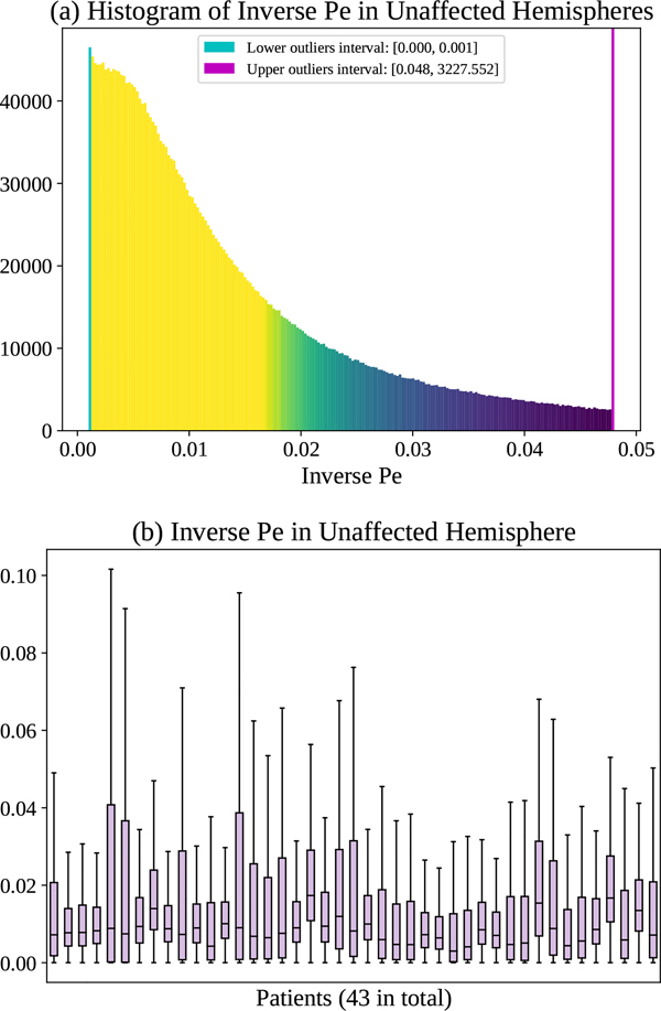
where ‖V‖₂, D are already defined based on our PIANO feature maps (Sec. ??), L is the characteristic length. Since the voxel spacings in PI are ≈ 1 mm, we set L to 1 mm for simplicity. By definition, Pe values range from 0 to ∞, indicating different process behavior, i.e., varying from pure diffusion, to diffusion-dominant transport, to advection-dominant transport, and lastly to pure advection. To achieve better visualizations for all kinds of mass transport, we compute both Pe and the inverse of Pe, with larger Pe (smaller inverse Pe) indicating the advection takes a larger portion and diffusion takes a smaller portion in the overall advection-diffusion process (and vice versa). Fig. ?? (a) and Fig. ?? (a) show the histograms of Pe and inverse Pe in the unaffected hemispheres of all patients. A small portion of voxels which have lower or higher values may indicate those regions where either advection or diffusion dominantes. Fig. ?? (b) and Fig. ?? (b) show the distributions of Pe and inverse Pe for each patient. Note that there is little across-patient variability with respect to the median of the inverse Pe.

Based on the above discussion about cerebral blood velocity and the Péclet number, the velocity and diffusion fields estimated by PIANO fall within reasonable value ranges, and are consistent with value ranges reported in literature as well.

VI. Further Discussions

A. PIANO and AIF-based Perfusion Measures

Although the parameters from PIANO and those from conventional deconvolution approaches (e.g., CBF) are all values derived from the contrast agent time-course, they measure different aspects of perfusion. Specifically, CBF focuses on the amount of blood flow passing through the brain tissue, while PIANO’s parameters are invariant to the overall blood flow amount: instead, they depend on the gradients of CA across space and time and assess how contrast agent flows and disperses throughout the brain. I.e., V & D will remain unchanged with varying amounts of transported CA. Specifically, for any $\alpha \in {\mathcal{R}}^{+}$:

$$\begin{gathered} \frac{\partial (\alpha C(\mathbf{x},t))}{\partial t}=-\mathbf{V}(\mathbf{x})\cdot \nabla (\alpha C(\mathbf{x},t)) \\ +\nabla \cdot (\mathbf{D}(\mathbf{x})\nabla (\alpha C(\mathbf{x},t))) \end{gathered}$$ (18)

the estimates remain unchanged⁶.

Note that PIANO measures are indeed different from AIF-based approaches; and we do not intend to capture standard AIF-based measures by PIANO. Instead, based on our advection-diffusion perspective, PIANO is able to provide additional useful measures, which we show to be effective in detecting lesion areas, while not relying on specifying an AIF. Hence, our goal is to supplement existing parameter maps computed from the conventional AIF-based methods.

B. PIANO’s Applicability to Other Perfusion Imaging Modalities

CT perfusion:

As PIANO models CA transport based on local concentration changes, it should in principle be directly applicable to CT perfusion images, once the Hounsfield units of CT perfusion images have been converted to CA concentrations [?].

Arterial Spin Labeling (ASL):

ASL measures are obtained very differently compared to CT perfusion and DSC-MR perfusion. Specifically, ASL perfusion measurements are usually based on only two time points [?]. Hence, PIANO would likely not be suitable for ASL as it relies on measurements of CA transport dynamics during all measured time intervals and requires higher temporal resolution.

C. Interpretation of PIANO’s Diffusion

As also mentioned in Sec. ??, the diffusion in PIANO captures the movements of freely-diffusive CA within the extracellular space or the macroscopic effect of capillary transport. It is important to note that because our voxel sizes (≈ 1 mm) are orders of magnitude larger than the capillary radii [?], capillary blood transport may manifest as diffusion macroscopically. Therefore, the diffusion estimated by PIANO should be considered a combined effect at voxel scale.

It is also important to note that the DWI-derived apparent diffusion coefficient (DWI-ADC) values are not expected to be similar to the diffusion values we estimate. DWI-ADC measures local water diffusion, whereas we measure how contrast agent is distributed throughout the brain and capture this distribution behavior via an advection-diffusion equation. This means, for example, that if a contrast agent does not reach certain parts of the brain (as might be the case for a stroke for example) velocity and diffusion values are expected to be low. In a sense this is a functional measurement (i.e., what is being reached by the contrast agent and how the contrast agent distributes), whereas DWI-ADC measures local tissue properties.

VII. Conclusions

We proposed PIANO which estimates the velocity and diffusion fields of CA transport via an advection-diffusion PDE. Unlike most postprocessing approaches which treat voxels independently, PIANO considers spatial dependencies and does not require estimating the AIF or deconvolution techniques. We demonstrate that PIANO can successfully resolve velocity and diffusion field ambiguities and results in sensitive measures for the assessment of stroke, comparing favorably to conventional measures of perfusion. Future work will explore thresholds based on statistical atlases and PIANO’s applicability to other PI modalities.

Fig. 1:

Toy example of 2D PIANO estimation. (a) Simulated advection-diffusion process with constant velocity and diffusivity; (b) Estimated advection-diffusion process from t = 0. PIANO successfully captures the advection-diffusion process.

Fig. 2:

Estimation framework of PIANO for one iteration (See Alg. ?? for the entire estimation approach), given training sample $S^i=\left\{C^{t_j}\mid j=i,i+1,\dots ,i+T_{\text{pd}}\right\}$.

Fig. 3:

PIANO effectiveness and robustness testing: box plots of mean absolute error (MAE). (a) Advection Imaging via Advection: MAE of estimated ‖V‖₂; (b) Diffusion Imaging via Diffusion: MAE of estimated D. To ensure that estimation errors can be compared across different patients, we scaled all estimated feature maps by the maximum value of the corresponding ground truth feature maps.

Fig. 4:

PIANO effectiveness and robustness testing: advection imaging via advection. Top row shows the ground truth ‖V^gt‖₂ used for simulating pure advection. (a)-(f) refer to the results for ‖V‖₂ estimated by PIANO, with simulated advection imaging series where Rician noise at levels 0%, 2%, 4%, 6%, 8%, 10% was added respectively.

Fig. 5:

PIANO effectiveness and robustness testing: diffusion imaging via diffusion. Top row shows D^gt used for simulating the ground truth pure diffusion. (a)-(f) refer to the results for D estimated from the ground truth pure diffusion image time-series where Rician noise at levels 0%, 2%, 4%, 6%, 8%, 10% was added respectively.

Fig. 6:

PIANO identifiability testing: advection imaging via advection-diffusion. Top row shows ‖V^gt‖₂ used for simulating ground truth pure advection. Rows below show the estimated ‖V^est‖₂ and D^est on corresponding slices. Note that the plotted value scale for D^est is 0.01 of that for ‖V^gt‖₂ and ‖V^est‖₂.

Fig. 7:

PIANO identifiability testing: diffusion imaging via advection-diffusion. Top row shows D^gt used for simulating ground truth pure diffusion. Rows below show the estimated D^est and ‖V^est‖₂ on corresponding slices. Note that the plotted value scale for ‖V^est‖₂ is 0.01 of that for D^gt and D^est.

Fig. 8:

PIANO feature maps for one stroke patient, where the lesion is located in the left hemisphere. Top row: segmented stroke lesion region (white) on different slices, obtained from ISLES 2017. The corresponding slices for the PIANO feature maps are shown in the following rows.

Fig. 9:

PIANO feature maps for another patient in the ISLES 2017 training set, where the lesion is located in the right hemisphere. Top row: segmented stroke lesion region (white) on different slices. The corresponding slices for the PIANO feature maps are shown in the following rows.

Fig. 10:

Histogram of mean absolute percentage error (MAPE) for PIANO’s concentration time-series prediction across 43 patients, computed across all predicted time points and over the entire brain region.

Fig. 11:

Comparison results between PIANO feature maps and ISLES 2017 maps (ADC, CBF, CBV, MTT, TTP, Tmax). (a) Box plots of the lesion-specific mean ratio (μ^r), lesion-specific STD ratio (σ^r); (b) Box plots of the lesion-specific absolute t-values (|t|) for all maps, computed from 43 patients. ⋆, ⋄, ○ indicate statistically significant differences between the PIANO feature maps and ISLES 2017 maps respectively, based on a paired t-test with Bonferroni correction at a significance level of 0.05; (c-d) Receiver operating characteristic (ROC) curves of all maps for lesion classification task thresholded based on actual parameter values (c) and ratios (d).

Fig. 12:

Predicted concentration time series for the same patient shown in Fig. ??, where (i)-(vi) correspond to slices #1–6 respectively. Each grouped row displays (a) the measured concentration image sequences, (b) the predicted concentrations and (c) the absolute error of predicted concentration at corresponding time points.

Fig. 13:

Predicted concentration time series for the same patient shown in Fig. ??, where (i)-(vi) correspond to slices #1–6 respectively. Each grouped row displays (a) the measured concentration image sequences, (b) the predicted concentrations and (c) the absolute error of predicted concentration at corresponding time points.

Fig. 14:

(a) Histogram of ‖V‖₂ in the unaffected hemispheres of 43 ISLES 2017 patients, and (b) corresponding box plots of distribution for individual patients.

Fig. 15:

(a) Histogram of Pe in the unaffected hemispheres of 43 ISLES 2017 patients, and (b) corresponding box plots of distribution for individual patients.

Fig. 16:

(a) Histogram of inverse Pe in the unaffected hemispheres of 43 ISLES 2017 patients, and (b) corresponding box plots of distribution for individual patients.

TABLE I:

Quantitative comparison between PIANO feature maps and ISLES 2017 maps over 43 subjects, using Mean, Median, Standard Deviation (STD) of the lesion-specific mean ratio μ^r, STD ratio σ^r (the lower the better), absolute t-value |t| (higher absolute value indicates greater difference), and area under curve (AUC) of receiver operating characteristic (ROC) curves (higher value means better segmentation performance) based on actual parameter values and ratio between hemispheres.

Maps		||V||2	D	ADC	CBF	CBV	MTT	TTP	Tmax
μr	Mean	0.54	0.59	0.76	0.57	0.72	0.61	0.69	0.21
	Median	0.52	0.56	0.78	0.56	0.76	0.63	0.68	0.15
	STD	0.12	0.19	0.14	0.19	0.15	0.20	0.13	0.16
σr	Mean	0.69	0.55	0.75	0.63	0.76	0.56	0.55	0.35
	Median	0.66	0.55	0.78	0.61	0.77	0.55	0.54	0.29
	STD	0.14	0.17	0.20	0.18	0.16	0.17	0.19	0.23
|t|	Mean	60.10	29.51	20.55	32.61	13.53	33.56	44.59	59.86
	Median	47.13	20.58	13.50	26.08	8.48	18.52	28.87	46.44
	STD	51.83	27.67	19.53	27.47	14.21	31.70	44.16	50.33
AUC	Actual	0.73	0.63	0.69	0.66	0.57	0.64	0.75	0.78
	Ratio	0.84	0.72	0.66	0.71	0.57	0.60	0.80	0.78

References

- [1].Fieselmann A, Kowarschik M, Ganguly A, Hornegger J, and Fahrig R, “Deconvolution-based CT and MR brain perfusion measurement: Theoretical model revisited and practical implementation details,” Journal of Biomedical Imaging, vol. 2011, 2011. [DOI] [PMC free article] [PubMed] [Google Scholar]
- [2].Petcharunpaisan S, Ramalho J, and Castillo M, “Arterial spin labeling in neuroimaging,” World journal of radiology, vol. 2, no. 10, pp. 384–398, 2010. [DOI] [PMC free article] [PubMed] [Google Scholar]
- [3].Grü ner JM, Paamand R, Hø jgaard L, and Law I, “Brain perfusion CT compared with 15O-H2O-PET in healthy subjects,” EJNMMI research, vol. 1, no. 1, 2011. [Online]. Available: https://pubmed.ncbi.nlm.nih.gov/22214473 [DOI] [PMC free article] [PubMed] [Google Scholar]
- [4].Demeestere J, Wouters A, Christensen S, Lemmens R, and Lansberg MG, “Review of perfusion imaging in acute ischemic stroke,” Stroke, vol. 51, no. 3, pp. 1017–1024, 2020. [DOI] [PubMed] [Google Scholar]
- [5].Mouridsen K, Christensen S, Gyldensted L, and Østergaard L, “Automatic selection of arterial input function using cluster analysis,” Magnetic Resonance in Medicine, vol. 55, no. 3, pp. 524–531, 2006. [DOI] [PubMed] [Google Scholar]
- [6].Schmainda K, Prah M, Hu L, Quarles C, Semmineh N, Rand S, Connelly J, Anderies B, Zhou Y, Liu Y, Logan B, Stokes A, Baird G, and Boxerman J, “Moving toward a consensus DSC-MRI protocol: Validation of a low–flip angle single-dose option as a reference standard for brain tumors,” American Journal of Neuroradiology, 2019. [DOI] [PMC free article] [PubMed] [Google Scholar]
- [7].Schmainda K, Prah M, Zhang Z, Snyder B, Rand S, Jensen T, Barboriak D, and Boxerman J, “Quantitative delta T1 (dT1) as a replacement for adjudicated central reader analysis of contrast-enhancing tumor burden: A subanalysis of the american college of radiology imaging network 6677/radiation therapy oncology group 0625 multicenter brain tumor...,” American Journal of Neuroradiology, 2019. [DOI] [PMC free article] [PubMed] [Google Scholar]
- [8].Cookson A, Lee J, Michler C, Chabiniok R, Hyde E, Nordsletten D, and Smith N, “A spatially-distributed computational model to quantify behaviour of contrast agents in MR perfusion imaging,” Medical Image Analysis, vol. 18, no. 7, pp. 1200–1216, 2014. [DOI] [PMC free article] [PubMed] [Google Scholar]
- [9].Harabis V, Kolar R, Mezl M, and Jirik R, “Comparison and evaluation of indicator dilution models for bolus of ultrasound contrast agents,” Physiological measurement, vol. 34, no. 2, pp. 151–162, 2013. [DOI] [PubMed] [Google Scholar]
- [10].Strouthos C, Lampaskis M, Sboros V, Mcneilly A, and Averkiou M, “Indicator dilution models for the quantification of microvascular blood flow with bolus administration of ultrasound contrast agents,” IEEE Transactions on Ultrasonics, Ferroelectrics, and Frequency Control, vol. 57, no. 6, pp. 1296–1310, 2010. [DOI] [PubMed] [Google Scholar]
- [11].Marín-Padilla M, “The human brain intracerebral microvascular system: development and structure,” Frontiers in neuroanatomy, vol. 6, p. 38, 2012. [DOI] [PMC free article] [PubMed] [Google Scholar]
- [12].Barbarosie C, “Representation of divergence-free vector fields,” Quarterly of Applied Mathematics, vol. 69, 2011. [Google Scholar]
- [13].LeVeque RJ, Finite Volume Methods for Hyperbolic Problems, ser. Cambridge Texts in Applied Mathematics. Cambridge University Press, 2002. [Google Scholar]
- [14].Perona P and Malik J, “Scale-space and edge detection using anisotropic diffusion,” IEEE Transactions on Pattern Analysis and Machine Intelligence, vol. 12, no. 7, pp. 629–639, 1990. [Google Scholar]
- [15].Weickert J, “Anisotropic diffusion in image processing,” pp. 15–25, 1998. [Online]. Available: https://www.mia.uni-saarland.de/weickert/Papers/book.pdf
- [16].Kistler M, Bonaretti S, Pfahrer M, Niklaus R, and Büchler P, “The virtual skeleton database: An open access repository for biomedical research and collaboration,” Journal of Medical Internet Research, 2013. [DOI] [PMC free article] [PubMed] [Google Scholar]
- [17].Maier O, Menze BH, von der Gablentz J, Hani L, Heinrich MP, Liebrand M, Winzeck S, Basit A, Bentley P, Chen L, Christiaens D, Dutil F, Egger K, Feng C, Glocker B, Götz M, Haeck T, Halme H-L, Havaei M, Iftekharuddin KM, Jodoin P-M, Kamnitsas K, Kellner E, Korvenoja A, Larochelle H, Ledig C, Lee J-H, Maes F, Mahmood Q, Maier-Hein KH, McKinley R, Muschelli J, Pal C, Pei L, Rangarajan JR, Reza SMS, Robben D, Rueckert D, Salli E, Suetens P, Wang C-W, Wilms M, Kirschke JS, amer UMK, Münte TF, Schramm P, Wiest R, Handels H, and Reyes M, “ISLES 2015 - a public evaluation benchmark for ischemic stroke lesion segmentation from multispectral MRI medical image analysis,” Medical Image Analysis, vol. 35, 2017. [DOI] [PMC free article] [PubMed] [Google Scholar]
- [18].Essig M, Shiroishi MS, Nguyen TB, Saake M, Provenzale JM, Enterline D, Anzalone N, Dörfler A, Rovira A, Wintermark M, and Law M, “Perfusion MRI: the five most frequently asked technical questions,” AJR. American journal of roentgenology, vol. 200, no. 1, pp. 24–34, 2013. [DOI] [PMC free article] [PubMed] [Google Scholar]
- [19].Meijering EHW, Niessen WJ, Pluim JPW, and Viergever MA, “Quantitative comparison of sinc-approximating kernels for medical image interpolation,” in Medical Image Computing and Computer-Assisted Intervention – MICCAI’99, Taylor C and Colchester A, Eds. Berlin, Heidelberg: Springer Berlin Heidelberg, 1999, pp. 210–217. [Google Scholar]
- [20].Aja-Fernandez S, Niethammer M, Kubicki M, Shenton ME, and Westin C, “Restoration of DWI data using a Rician LMMSE estimator,” IEEE Transactions on Medical Imaging, vol. 27, no. 10, pp. 1389–1403, 2008. [DOI] [PMC free article] [PubMed] [Google Scholar]
- [21].Ivanov K, Kalinina M, and Levkovich Y, “Blood flow velocity in capillaries of brain and muscles and its physiological significance,” Microvascular Research, vol. 22, no. 2, pp. 143–155, 1981. [DOI] [PubMed] [Google Scholar]
- [22].Zhang P, Huang Y, Li Y, Lu M, and Wu Y, “A large-scale study on relationship between cerebral blood flow velocity and blood pressure in a natural population,” Journal of Human Hypertension, vol. 20, no. 10, pp. 742–748, 2006. [DOI] [PubMed] [Google Scholar]
- [23].Bouvy WH, Geurts LJ, Kuijf HJ, Luijten PR, Kappelle LJ, Biessels GJ, and Zwanenburg JJM, “Assessment of blood flow velocity and pulsatility in cerebral perforating arteries with 7-T quantitative flow MRI,” NMR in Biomedicine, vol. 29, no. 9, pp. 1295–1304, 2016. [DOI] [PMC free article] [PubMed] [Google Scholar]
- [24].Franca LP, Frey SL, and Hughes TJ, “Stabilized finite element methods: I. application to the advective-diffusive model,” Computer Methods in Applied Mechanics and Engineering, vol. 95, no. 2, pp. 253–276, 1992. [Google Scholar]
- [25].Haller S, Zaharchuk G, Thomas DL, Lovblad KO, Barkhof F, and Golay X, “Arterial spin labeling perfusion of the brain: Emerging clinical applications,” Radiology, vol. 281, no. 2, pp. 337–356, 2016. [DOI] [PubMed] [Google Scholar]